Generalized Matrix Decomposition Regression: Estimation and Inference for Two-way Structured Data

UW Biostatistics Working Paper Series Winter 12-23-2019

Generalized Matrix Decomposition Regression: Estimation and

Generalized Matrix Decomposition Regression: Estimation and

Inference for Two-way Structured Data

Inference for Two-way Structured Data

Yue Wang Ali Shojaie Tim Randolph Jing Ma

Follow this and additional works at: https://biostats.bepress.com/uwbiostat

Part of the Biostatistics Commons, Multivariate Analysis Commons, Statistical Methodology Commons, and the Statistical Theory Commons

This working paper is hosted by The Berkeley Electronic Press (bepress) and may not be commercially reproduced without the permission of the copyright holder.

Generalized Matrix Decomposition Regression:

Estimation and Inference for Two-way Structured Data

Yue Wang, Ali Shojaie, Timothy W. Randolph and Jing Ma

December 31, 2019

Abstract

Analysis of two-way structured data, i.e., data with structures among both vari-ables and samples, is becoming increasingly common in ecology, biology and neuro-science. Classical dimension-reduction tools, such as the singular value decomposition (SVD), may perform poorly for two-way structured data. The generalized matrix de-composition (GMD, Allen et al., 2014) extends the SVD to two-way structured data and thus constructs singular vectors that account for both structures. While the GMD is a useful dimension-reduction tool for exploratory analysis of two-way structured data, it is unsupervised and cannot be used to assess the association between such data and an outcome of interest. In this article, we first propose the GMD regres-sion (GMDR) as an estimation/prediction tool that seamlessly incorporates two-way structures into high-dimensional linear models. The proposed GMDR directly re-gresses the outcome on a set of GMD components, selected by a novel procedure that guarantees the best prediction performance. We then propose the GMD inference (GMDI) framework to identify variables that are associated with the outcome for any model in a large family of regression models that includes GMDR. As opposed to most existing tools for high-dimensional inference, GMDI efficiently accounts for pre-specified two-way structures and can provide asymptotically valid inference even for non-sparse coefficient vectors. We study the theoretical properties of GMDI in terms of both the type-I error rate and power. We demonstrate the effectiveness of GMDR and GMDI on simulated data and an application to microbiome data.

Keywords: Dimension reduction; high-dimensional inference; prediction; two-way struc-tured data

1

Introduction

Analysis of two-way structured data, i.e., data with structures among the variables (columns) and among the samples (rows), is becoming increasingly common in ecology, biology and neuroscience. Often these two-way structures can be identified, at least partially, a priori. For example, a sample-by-taxon abundance data matrix in a microbiome study may have columns structured by the phylogeny of taxa and rows structured by an ecologically defined distance between samples. In neuroimaging studies involving functional MRI (fMRI) data, three-dimensional brain images are measured over time with high spatial resolution; here row structures exist as spatial dependencies across voxels and column structures exist as temporal patterns over time.

Two-way structured data can be summarized by three matrices: (i) an n ˆp data matrix X with n samples and p variables, (ii) an nˆn positive semi-definite (PSD) ma-trix H characterizing the row structures and (iii) a pˆp PSD matrix Q characterizing the column structures. Classical dimension-reduction tools, such as principal component analysis (PCA) and singular value decomposition (SVD), upon which PCA is based, are frequently used for exploratory analysis of unstructured data, but may perform poorly for structured data. Currently, there are two primary approaches that account for various types of structures in the data. One approach imposes constraints on the construction of the PC vectors. For example, the constraints enforce sparsity, as in the sparse PCA (Zou et al., 2006), or encourage smoothness, as in the functional PCA (Besse and Ram-say, 1986; Ramsay and Dalzell, 1991; Boente and Fraiman, 2000; James et al., 2000; Cai and Hall, 2006). The other approach consists of methods that account for more arbitrary structures that are pre-specified in matrices such as H and/or Q. These include multidi-mensional scaling (MDS, Mead, 1992), which amounts to PCA on H, and the generalized

SVD (GSVD, Van Loan, 1976; Paige and Saunders, 1981) or the generalized PCA (gPCA, Purdom, 2011), where the singular vectors inherit structure fromQ. In addition, the gener-alized matrix decomposition (GMD, Escoufier, 1987; Allen et al., 2014) provides a two-way decomposition based on both row and column structures, which directly generalizes SVD to two-way structured data. More specifically, the GMD of X with respect to H and Q, X“USVT, is obtained by solving the following optimization problem:

argmin_U,S,V}X´USVT}H,Q, (1)

subject to UT_{HU “ I}

K,VTQV “ IK and S “ diagpσ1, . . . , σKq. Here, K is the rank

of XTHXQ and }M}2H,Q “ trpMTHMQq for any matrix M P Rnˆp. The GMD directly

extends SVD by replacing the Frobenius norm with theH,Q-norm} ¨ }H,Q. As such, GMD

preserves appealing properties of SVD such as ordering the component vectors according to a nonincreasing set of GMD values, σ1, . . . , σK, indicating that the decomposition of the

total variance of X into each dimension is nonincreasing.

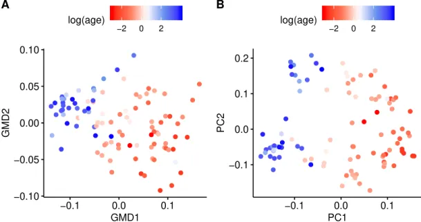
The GMD is a powerful tool for exploratory analysis of two-way structured data. Fig. 1A is a beta diversity plot ofn“100 human microbial abundance vectors withp“149 taxa based on data from Yatsunenko et al. (2012). The structure among taxa is characterized by a similarity kernel derived from the patristic distance between each pair of the tips of the phylogenetic tree. The structure among samples derives from their pairwise Euclidean dissimilarity based on bacterial gene groups found in each sample—counts of bacterial genes were combined into functional groups according to KEGG Enzyme Commission (EC) numbers; see Yatsunenko et al. (2012). The two axes in Fig. 1A are the first two columns of the right GMD vectorsV, obtained by solving (1) with respect to both structures. Each sample is then configured by the coordinates of the projection of each microbial abundance

−0.10 −0.05 0.00 0.05 0.10 −0.1 0.0 0.1 GMD1 GMD2 −2 0 2 log(age) A −0.1 0.0 0.1 0.2 −0.1 0.0 0.1 PC1 PC2 −2 0 2 log(age) B

Figure 1: Beta diversity plots of data from Yatsunenko et al. (2012). (a): Beta diversity plot constructed using the GMD vectors with respect to both row and column structures. (b): Beta diversity plot constructed from the SVD vectors.

vector onto the two axes, and is colored by the logarithm of the subject’s age. As a reference, Fig. 1B shows the configuration of samples by using the right singular vectors of the SVD of the data matrix. Comparing Fig. 1A with Fig. 1B, it can be seen that the GMD vectors provide a different two-dimensional configuration of subjects than the SVD, which ignores row and column structures. This is explored further in Wang et al. (2019) using a GMD-biplot while in Section 5, these data are used to illustrate the advantages of incorporating two-way structures for the prediction of age and estimation/inference of individual taxa associated with age. Indeed, our first contribution in this paper is introducing the GMD regression (GMDR), a prediction tool that seamlessly incorporates these two-way structures into a regression framework. The GMDR generalizes the well-known principal component

regression (PCR) for two-way structured data by regressing the outcome on a set of GMD components. However, unlike PCR, our GMDR selects the GMD components that are most predictive of the outcome, which may not be those corresponding to the largest GMD values. This novel selection procedure ensures more accurate prediction using GMDR.

Despite their advantages in terms of prediction, a key limitation of regression frame-works based on dimension reduction, including PCR and its generalization via GMDR, is their limited interpretability. In fact, PCR is seldom used for estimating the regression co-efficients, and to the best of our knowledge, no formal inferential procedure that can assess the significance of individual variables has been proposed for PCR. Our second contribution addresses this limitation: We define the GMDR estimator of the regression coefficients and further link it to a broad class of estimators that includes many existing regularized meth-ods which incorporate, to varying degrees, structures among the samples and variables. We also introduce the GMD inference (GMDI) framework, a high-dimensional inferential pro-cedure that assesses the significance of individual variables based on an arbitrary estimator in this class.

GMDI has the following appealing features. First, it does not require the regression co-efficients to be sparse; rather, our constraints are imposed with respect to the pre-specified structures, which are often more natural in practice. Existing high-dimensional inferential methods, including Zhang and Zhang (2014); B¨uhlmann (2013); van de Geer et al. (2014); Zhao and Shojaie (2016); Ning and Liu (2017) and Chernozhukov et al. (2015), all require sparse coefficients, which may not hold when column structures exist. An extreme exam-ple is the setting of highly correlated variables (Hebiri and Lederer, 2013); in this case, if one variable is significant, others may be significant too. An example of a potentially non-sparse regression coefficient vector is discussed in the analysis of the microbiome data

illustrated in Fig. 1 in Section 5. Second, GMDI does not require the precision matrix of the vector of variables to be sparse. Although the non-sparse high-dimensional inferential tool proposed by Zhu and Bradic (2018) does not require sparse signals, it does require the precision matrix of the vector of variables to have row sparsity for the purpose of assessing the significance of individual variables. Hence, their assumptions are tailored to a specific type of structured data, which may not hold for arbitrary two-way structured data. Fi-nally, GMDI allows dependent and heteroscedastic samples. In contrast, the vast majority of existing high-dimensional inferential procedures require i.i.d. samples, which are not expected when row structures exist.

The proposed GMDI follows the general idea of bias correction for ridge type estima-tors, as first considered in B¨uhlmann (2013). However, as mentioned earlier, GMDI is not limited to GMDR, and it applies to a broad class of existing models, including the ker-nel penalized regression (KPR, Randolph et al., 2018) and the generalized ridge regression (Hemmerle, 1975; Randolph et al., 2012), for which corresponding inferential tools are lack-ing. Moreover, unlike B¨uhlmann (2013) which only corrects the projection bias that arises when n ă p, GMDI corrects both the projection bias and the estimation bias that arises

from the selection of GMD components for GMDR, or the choice of tuning parameter for KPR. We derive the asymptotic distribution of the bias-corrected estimator. Based on this, we construct asymptotically valid two-sided p-values and provide sufficient conditions un-der which GMDI offers guaranteed power. Our numerical studies demonstrate the superior performance of GMDI for two-way structured data compared to existing high-dimensional inferential methods, even when pre-specified structures are not fully informative.

The rest of the article is organized as follows. In Section 2, we first introduce the GMDR estimation/prediction framework, accompanied by the novel selection procedure of

the GMD components. We then link the GMDR estimator to a broad class of estimators. In Section 3, we present the GMDI procedure for any arbitrary estimator in this class and explain the rationale underlying the key assumptions that are required for GMDI. Simulation studies that examine the finite-sample performance of GMDI are presented in Section 4. In Section 5, we demonstrate the effectiveness of GMDR and GMDI on an application to microbiome data which are illustrated in Fig. 1. Section 6 summarizes our findings and outlines potential extensions. Technical proofs are provided in the Appendix.

2

The GMDR Estimation

We first introduce some notations that will be used throughout the article. We use normal letters to denote scalars, bold lowercase letters to denote vectors and bold uppercase letters to denote matrices. For any vector v P Rp, we use vj to denote the j-th element of v for j “1, . . . , p. For any matrix MP Rnˆp, let mj and mij denote the j-th column and pi, jq

entry ofM, respectively fori“1, . . . , nand j “1, . . . , p. For any index setI P t1, . . . , pu,

letvI andMIdenote the subvector ofvwhose elements are indexed byIand the submatrix

ofMwhose columns are indexed byI, respectively. M´_{denotes the Moore-Penrose inverse}

of M. Let IpAq denote the indicator function of the event A; i.e, IpAq “ 1 if A is true, and IpAq “ 0 otherwise. Finally, we let }v}0 “ řp_j“1Ipvj ‰ 0q, }v}q “

´ řp

j“1|vj|

q¯1{q

for any 0 ăq ă 8, }v}8 “maxj|vj|, }v}2K “vTKv for any PSD matrix K, and }M}q “

sup_}v}q“1}Mv}q for any qą0.

Suppose we observetxi, yiufor i“1, . . . , n, where xi P Rp is a pˆ1 vector of variables

we consider the following model

y“Xβ˚`, (2)

whereβ˚

“ pβ1˚, . . . , βp˚qis apˆ1 vector of unknown parameters characterizing the

relation-ship between X and y. Let H P Rnˆn and QP Rpˆp be two PSD matrices characterizing

structures among samples and variables, respectively.

We assumeX,HandQare deterministic. LettingH“LHLHT andr“LH T

, we also assume that _r1, . . . ,rn are i.i.d. random variables with mean 0 and variance σ

2

. This is a

natural assumption astCovpqu´1, which is equal toH(up to a constant), characterizes the structure among samples. In Section 3.2, we provide an alternative, albeit more restrictive, view of X, H and Q, wherein X arises from a matrix-variate model (Allen et al., 2014) with separable row covariance H´ _{and column covariance Q}´_{. We consider p}

“ ppnq and

allow p to be greater than n. Thus (2) is essentially a high-dimensional linear model. Finally, throughout the article, we assume that X and y are appropriately centered such that 1T

nHy “0 and1TnHX“0T, where1n is an nˆ1 vector of all ones.

Recall that (1) defines the GMD of X with respect to Hand Q. Unlike the SVD, the GMD matrices U and V are not orthogonal in the Euclidean norm unless H “ In and Q “Ip. An efficient algorithm was proposed by Allen et al. (2014) to iteratively solve for

each column of U,Sand V in (1). Analogous to the SVD of X, which is closely related to the eigen-decomposition ofXT_{X, the GMD of Xwith respect to Hand Qis related to the}

eigen-decomposition of XT_{HXQ. In fact, Escoufier (1987) and Allen et al. (2014) show}

that the squared GMD valuesσ2

1, . . . , σK2 are non-zero eigenvalues ofXTHXQand columns

of Vare the corresponding eigenvectors. Note thatXT_{HXQmay not be symmetric, again}

implying that columns of V may not be orthogonal in the Euclidean norm. Given V and S, the nˆK matrix Ucan be uniquely defined by US“XQV.

To estimate β˚, our GMDR regresses y on a reduced subset of GMD components. More specifically, let νj “ ujσj be the j-th GMD component for j “ 1, . . . , K and set Υ “ pν1, . . . ,νKq PRnˆK. For any pre-determined index set I Ă t1, . . . , Ku, the GMDR

estimator of β˚_, p

β_GMDRpIq, can be obtained in two steps:

(i) Regress y onΥI and obtain γppIq “argminγ}y´ΥIγ}

2

H.

(ii) Calculate βp

GMDRpIq “ pQVqIγppIq.

Letting wj “Ipj PIq for j “1, . . . , K, βp_GMDRpIq can be explicitly expressed as

p

βGMDRpIq “QVWIS

´1_UT_{Hy, (3)}

where WI “diagpw1, . . . , wKq.

To achieve the best prediction performance, it is critical to select the “optimal” index set I. First, note that if Q “Ip and H “In, then GMDR reduces to PCR. Thus, analogous

to PCR, a natural way to select I is to consider GMD components that correspond to large GMD values, refered to as top GMD components hereafter. However, there is a long historical debate on the rationale behind selecting top PCs for PCR, because it is well known that in finite samples, top PCs are not necessarily more predictive of the outcome than tail PCs; see Cook (2007) and the references therein for more discussions.

A natural question arises: how to find the “optimal” I from all subsets of t1, . . . , Ku

that leads to the best prediction performance? Note that an exhaustive search over all 2K

subsets of t1, . . . , Ku is computationally infeasible even for moderate K. To address this

problem, we propose a procedure that weighs the importance of each GMD component by its contribution to the prediction of the outcome. Our idea is to decompose the total R2

of the model into K terms, each corresponding to a GMD component. More specifically, we first regress y on all GMD componentsΥ with respect to the H-norm, and obtain

p

γ “argmin_γ}y´Υγ}2_H. (4)

It can then be seen that the totalR2 _{for the model is given byR}2 _{“ }Υ}

p

γ}2_H{ }y}2_H. Letting

p

γ “ pγp1, . . . ,pγKq T

, we can write R2 “řK_j“1r2_j, where

r_j2 “ }νjpγj} 2 H }y}2_H “ σ_j2_pγ_j2 }y}2_H, for j “1, . . . , K.

Here, we use the fact that νT

i Hνj “ 0 for any i ‰ j. Since r21, . . . , rK2 share the same

denominator, we define thevariable importance (VI) score of thej-th GMD component as VIj “σj2pγ

2

j for j “1, . . . , K, with a higher score being more predictive of the outcome.

Based on VI1, . . . ,VIK, we select the optimal I in three steps:

(i) Sort tVIj :j “1, . . . , Ku in nonincreasing order: VIj1 ěVIj2 ě ¨ ¨ ¨ ěVIjK.

(ii) For eachk “1, . . . , K, considerIk “ tj1, . . . , jkuand calculate the generalized

cross-validation (GCV) statistic: GCVpkq “ }pIn´Gpkqqy} 2 H ptrpIn´Gpkqqq2 “ }pIn´Gpkqqy} 2 H pn´kq2 , where Gpkq “ ΥIk ` ΥT_I kHΥIk ˘´1 ΥT_I kH.

(iii) Find kopt “argminkGCVpkq, and the optimum I asIkopt “ tj1, . . . , jkoptu.

Having selected the optimal GMD components, we now return to the estimation of regression coefficients. It can be seen from (3) that our GMDR estimatorβp

GMDRpIqbelongs

to the following class of estimators:

BGMD “ tβ w

PRp :βw “QVWS´1_UT_Hy

u, (5)

where W “ diagpw1, . . . , wKq and wj ě 0 for j “ 1, . . . , K. Besides selecting each wj as

either 0 or 1, as done for GMDR, one can instead let wj depend on a tuning parameter η.

For example, letting wj “ wjpηq “ pσj2 `ηq´2σj2 and Wη “ diagpw1pηq, . . . , wKpηqq, one

can obtain another estimator in BGMD asβ w

pηq “ QVWηS´1UTHy. If bothHand Q are

non-singular, we can see that (see Section (A1) in the Appendix)

βwpηq “ argmin_β}y´Xβ}2_H`η}β}2_Q´1 :“βp_KPRpηq, (6)

where βp_KPRpηq is the estimator of the kernel penalized regression (KPR, Randolph et al.,

2018). KPR is a general framework for two-way structured regression, and covers many existing approaches, including Hemmerle (1975) and Randolph et al. (2012). Although the motivations behind KPR and GMDR are quite different, (6) implies that they share many features. First, both βp_GMDRpIq and βp_KPRpηq are in the column space of Q, indicating both

estimators incorporate information from Q in similar ways. Second, both estimators exert shrinkage effects on the GMD components through the weight matrix W. The difference is that, βp_GMDRpIqexerts discrete shrinkage by truncation, nullifying the contribution of the

GMD components that are not selected, while βp_KPRpηq exerts a smooth shrinkage effect

through the tuning parameter η inherently involved in its construction. This connection between GMDR and KPR is similar to that between PCR and the ridge regression (Hoerl and Kennard, 1970).

3

The GMD Inference

In this section, we propose a high-dimensional inferential framework, called the GMD infer-ence (GMDI), for the entire class of models BGMD, given in (5). This inferential procedure

and its theoretical properties are presented in Section 3.1. In Section 3.2, we provide the rationale behind the key assumptions. Recall model (2) as y“Xβ˚`, where“LHTr

and_r“ pr1, . . . ,rnq

T_{. From now on, we assume that}

r1, . . . ,rn are i.i.d.sub-Gaussian with

mean 0 and variance σ2; that is, there exists a constant C ą0 such that

Epexppt_riqq ďexp ˆ

Cσ2t2

2

˙

for all tPR and i“1, . . . , n. (7)

Assumption (7) is less restrictive than the Gaussianity assumed in B¨uhlmann (2013) and Zhang and Zhang (2014). Nonetheless, sub-Gaussianity is only considered for ease of presentation; our results can be easily extended to other distributions with certain tail bounds, such as sub-exponential distributions (Chapter 2, Wainwright, 2019).

3.1

The GMDI Procedure

Let βw “ pβ1w, . . . , βpwq be an arbitrary estimator from BGMD in (5) with the weight matrix

W. Our goal is to test the null hypothesis H0,j :βj˚ “0 for somej “1, . . . , p, where β ˚

is defined in (2). We first note that βw

j may be a biased estimator of βj˚. Letting Bj denote

the bias of βw

j , it can be seen that

Bj “ ` QVWVTβ˚˘ j ´β ˚ j “ ÿ m‰j ξ<sub>jm</sub>w β˚ m` pξ w jj´1qβ ˚ j, 12

where ξ_jmw “ pQVWVTqpj,mq, for j, m“ 1, . . . , p. To construct a test statistic for testing

H0,j based on βjw, we correct the bias Bj by using an initial estimator that accurately

estimates β˚. Under H0,j, it can be seen that for anyhj PR,

Bj “Bjphjq:“ ÿ m‰j ξ_jmw β˚ m`hjpξjjw ´1qβ ˚ j.

With an initial estimator βinit “ pβinit

1 , . . . , βpinitqT that will be discussed later, we can

estimate Bjphjq by p Bjphjq “ ÿ m‰j ξ_jmw β_minit`hjpξjjw ´1qβ init j . (8)

Our bias-corrected estimator is defined as follows.

Definition 3.1. Let ry “ LH T

y denote the transformed outcome. For j “ 1, . . . , p, the bias-corrected estimator of β˚ j is of the form p β_jwphjq “ βjw´Bpjphjq “ n ÿ i“1 ajiyri´Bpjphjq, (9) where aji “ ` QVWS´1_UT_L H ˘ pj,iq, for i“1, . . . , n.

Remark 3.1. Letθ˚ _{be the projection ofβ}˚ _{onto the column space ofQV. Whenp}

ąn,Bj

can be decomposed as the sum of the estimation and projection biases, respectively, given by

`

QVWVTβ˚˘

j´θj andθj´β ˚

j.Unlike B¨uhlmann (2013) that only corrects the projection

bias, i.e., θj ´βj˚, we provide tighter bias correction by correcting both the estimation and

projection biases.

Remark 3.2. The two most intuitive choices of hj are 0 and 1, which are, respectively,

Bjp0q, one only corrects the bias under the null hypothesis, while if Bjp1q is considered,

one corrects the general bias regardless of β˚

j. Our bias-corrected estimator (9) generalizes

these two choices.

The following result characterizes the asymptotic distribution of βp_jwph_jqas nÑ 8.

Proposition 3.1. For j “1, . . . , p, consider the bias-corrected estimator βp_jwph_jq, given in

(9). If lim nÑ8 maxi“1,...,n|aji| řn i“1a2ji “0, (10)

then for all hj PR,

p β_jwphjq “ ` p1´hjqξwjj`hj ˘ β˚ j ` ÿ m‰j ξw<sub>jm</sub>pβm˚ ´β init m q `hjpξjjw ´1qpβ ˚ j ´β init j q `Z w j . (11) Here, Z_jw a σ2 Ωwjj d ÑNp0,1q as n Ñ 8, where Ωw_jj “ K ÿ l“1 $ & % w2_lσ´2 l ˜ _p ÿ t“1 qjtvtl ¸2, . -.

As shown in (9),aji is the weight for the i-th transformed outcome ryi in the definition

of βp_jwph_jq. Since Covpy_rq “ σ2I_n, condition (10) may thus imply that more information

can be obtained as more samples are collected. The following corollary of Proposition 3.1 serves the basis for testing H0,j :βj˚ “0.

Corollary 3.1. Assume (i) Ωw

jj ą 0 and (ii) }β ˚

´ βinit}1 is negligible. Then, under

condition (10), |σ´1 ` Ωw jj ˘´1{2 p βw

j phjq| is an asymptotically valid test statistic for testing H0,j.

The proofs of Proposition 3.1 and Corollary 3.1 are given in Section (A2) in the Ap-pendix. It can be easily checked that Ωw_jj ą0 is satisfied if and only if

max lPtl:ωlą0u ˜ _p ÿ t“1 qjtvtl ¸2 ą0. (12)

For the trivial case where Q “ Ip, (12) reduces to maxlPtl:ωlą0uvjl2 ą 0, which matches

condition (2.5) in B¨uhlmann (2013).

To obtain a βinit that can yield negligible }βinit ´β˚}1, we first introduce some

ad-ditional notations. Let Q“D∆DT denote the eigen-decomposition of Q, where ∆ “

diagpδ1, . . . , δqq and q is the rank of Q. Denote by PQ “ QQ´ “ DDT the

orthogo-nal projection onto the column space of Q. We assume that the following conditions are satisfied.

(A1) pIp´PQqβ˚ “0.

(A2) }DTβ˚}0 ďs0, wheres0 “o

`

n{logp˘r( for some rP p0,1{2q.

(A3) For some compatibility constant φ0,ną0 satisfying lim infnÑ8φ0,n ą0,

1 n}XD∆ 1{2_v }2_H ě φ 2 0,n s0

}vS˚}2₁ for all vP_Rq such that }v_´S˚}₁ ď3}v_S˚}₁, (13)

where S˚ _{is the support ofD}T_β˚_.

eigenvectors of Q, and (A3) is a compatibility condition on X with respect to H and Q. We explain the rationale behind (A1)–(A3) in Section 3.2.

Under assumptions (A1)–(A3),βinit is constructed in two steps:

(i) Find r βpλq “argmin_β p2nq´1}y´XDβ}2_H`λ››∆´1{2β › › 1 ( . (14)

(ii) Define βinit “Dβrpλq.

Here, the coefficient p2nq´1 in (14) is chosen for theoretical convenience and λ ą 0 is a tuning parameter. Letting ζjphjq “

ř m‰jξ

w

jmpβm˚ ´βminitq `hjpξjjw ´1qpβj˚´βjinitq for j “

1, . . . , pandΞ“diagpξw

11, . . . , ξppwq, the following result shows that the type-I error of testing H0,j can be asymptotically controlled using a test statistic based on the bias-corrected

estimator βp_jwph_jq given in (11). In the following theorems, without loss of generosity, we

assume that Q is appropriately scaled such that }Q}2 “1.

Theorem 3.1. Suppose the columns of X are standardized such that }Xdj}2H “ n, for

j “ 1, . . . , p. For βrpλq in (14), choose λ “ σ a

κn´1_{logp2pq for some κ ąC, where C is}

given in (7). Further denote for all hj PR,

Ψjphjq “σ › › › › ” ` QVWVT ´ p1´hjqΞ´hjIp ˘ D∆1{2ı pj,¨q › › › › 8 ˆ logp n ˙1{2´r ,

where for any matrix M, Mpj,¨q denotes the j-th row of M. Then, under condition (10)

and assumptions (A1)–(A3), limnÑ8Prp|ζjphjq| ď Ψjphjqq “1. Furthermore, under H0,j,

for any αą0, lim sup nÑ8 Pr ´ˇ ˇ ˇβp w j phjq ˇ ˇ ˇąα ¯ ďlim sup nÑ8 Pr`ˇˇZ<sub>j</sub>w ˇ ˇ`Ψ_jph_jq ąα ˘ . (15) 16

The result in (15) implies that, if Ωw_jj ą 0, we can test H0,j using the asymptotically

valid two-sided p-value

P_jwphjq “ 2 ¨ ˚ ˝1´Φ » — – !ˇ ˇ ˇβp w j phjq ˇ ˇ ˇ´Ψjphjq ) ` a σ2 Ωwjj fi ffi fl ˛ ‹ ‚, (16)

where Φp¨qis the cumulative distribution function of the standard normal distribution and

a` “maxpa,0q. In practice, to calculate the p-value in (16), we need an estimatepσ ofσ.

The p-value will still asymptotically control the type-I error if Prppσěσq Ñ1 as nÑ 8.

We estimate σ by theorganic lasso estimatorσppλq (Yu and Bien, 2019), whereλą0 is

a tuning parameter. We can apply their framework directly if we consider the transformed outcome ry “ LH

T

y and the transformed design matrix Xr “ L_HTXD. As shown in Yu

and Bien (2019), under some mild conditions, _pσ2

pλq is a consistent estimator of σ2 with λě p2κn´1logpq

1{2

for any κ ą1.

Remark 3.3. Theorem 3.1 is similar to Theorem 2.3 in Zhao and Shojaie (2016). How-ever, a notable difference is that our bound Ψjphjq depends on σ, whereas theirs does not.

Although this difference may seem trivial, incorporating σ into Ψjphjq actually accounts

for the scale of the outcome y. In other words, our bound Ψjphjq will change its scale

according to the scale of the outcome, which is more meaningful than the scale-independent bound in Zhao and Shojaie (2016).

Our next result guarantees the power of GMDI when the size of the true regression coefficient is sufficiently large.

Theorem 3.2. Assume the conditions of Theorem 3.1 hold and Ωw

some 0ăαă1 and 0ăψ ă1 such that ˇ ˇβ_j˚ ˇ ˇě |p1´h_jqξ_jjw `h<sub>j</sub>|´1¨ ´ 2Ψjphjq ` ` qp1´α{2q`qp1´ψ{2q ˘b σ2 Ωwjj ¯ , (17)

where Φpqtq “ t for any tP p0,1q, then

lim

nÑ8PrpP w

j phjq ďαq ěψ.

It should be noted that condition (17) may not hold whenp1´hjqξjjw`hj “0; however,

this rarely happens and can be easily checked in advance. In cases where (17) is not true, a different hj can be used.

3.2

Rationale behind Assumptions (A1)–(A3)

In this section, we motivate Assumptions (A1)-(A3) from two distinct perspectives.

We first consider a scenario whereX arises from a matrix-variate model with separable row covariance H´1 _{and column covariance Q}´1_{; that is, CovpvecpXqq “ Q}´1 _bH´1_,

where b denotes the Kronecker product and vecpXq denotes the npˆ1 vector obtained

by stacking the columns of X. In this scenario, besides using BGMD to estimate β

˚ _{in (2),}

an alternative approach is to first decorrelate the data, and then model the decorrelated data using existing tools for unstructured data. More specifically, recall H “ LHLHT,

Q“D∆DT, yr “LH

T_{y and} r

X “ LHTXD. Consider the relationship between yr and Xr

modeled by y_r“Xrβr ˚

`r. A straightforward derivation yields that

CovpvecpXrqq “∆´1bI_n and _r„Np0, σ2I_nq.

This indicates that the decorrelated data have trivial row and column structures; that is, the variables are uncorrelated and the samples are independent. As such, it is natural to assume that only a few coefficients in βr

˚

are non-zero when p is large. Moreover, it is easy to see that β˚

“ Dβr ˚

. This implies that pI´PQqβ˚ “ 0 and DTβ˚ is sparse,

which corresponds respectively to Assumptions (A1) and (A2). Assumption (A3) is then equivalent to a compatibility condition for the decorrelated data Xr (van de Geer et al.,

2009), which is a standard condition in high-dimensional inference.

This relationship between two-way structured data and the corresponding decorrelated data begs the question: why not work with the decorrelated data, get an estimator of βr

˚

, and then estimate β˚ _{according toβ}˚

“Dβr ˚

? While this may be valid for prediction, it is not a satisfying approach for inference. There are at least two reasons against working with decorrelated data. First, one would need to know the exact row and column covariance of X in order to “truly” decorrelate the data. However, this is unrealistic in general, and is not necessary for our GMDI; in fact, GMDI only requires that X satisfies a compatibility condition with respect to H, and that Q informs β˚ through a subset of its eigenvectors. Second, one may apply existing high-dimensional inferential tools to obtain p-values for the individual coefficients of βr

˚

, yet it is still not clear how to obtain p-values for the coefficients of β˚_{, which is our primary goal.}

Given the limitations of decorrelation discussed above, we next provide a second per-spective that directly explores the link between Assumptions (A1)–(A3) and the bias of an arbitrary estimator βw P BGMD. More specifically, note that the bias of β

w

“

QVWS´1_UT_{Hy is given by}

Recall that PQ denotes the orthogonal projection onto the column space of Q, and thus

for any β˚

PRp, we can write

β˚ “PQβ˚` pIp ´PQqβ˚.

Then, (18) can be expressed as

Biaspβwq “ Q`VWVTQ´Ip ˘ Q´_β˚ ``QVWVT ´Ip ˘ pIp´PQqβ˚. (19)

We make the following observations from (19).

(O1) Consider K “ p and assume Q is non-singular. Let βw be the GMDR estimator

with all GMD components selected. In this case, W“Ip and it can be seen that

VWVT_Q

“ Ip. Thus, we have Biaspβwq “ 0. This demonstrates that in the

low-dimensional case (K “pďn), the GMDR estimator based on all GMD components is an unbiased estimator of β˚ _{for any β}˚

PRp.

(O2) ConsiderK ăpand assumeQis non-singular, a common scenario in high-dimensional settings (n ăp). In this case, it is easy to see that PQ “Ip but VWVTQ ‰Ip for

any W. Then, for fixed Q and W,

}Biaspβwq}₂ ď }Q}₂››VWVTQ´I_p › › 2 › ›Q´1β˚ › › 2,

indicating that βw is less biased if }Q´1_β˚

}₂ is small. Furthermore, recall that

Q“D∆DT is the eigen-decomposition of Q. It can be seen that › ›Q´1β˚ › › 2 2 “ q ÿ j“1 δ´2 j ` dT_jβ˚˘2. (20)

Since δ1 ě ¨ ¨ ¨ ěδq, (20) implies that βw is less biased if the following two conditions

hold: (i) only a few dT jβ

˚ _{are non-zero, and (ii) for largej (small δ}

j), dTjβ ˚

“0.

(O3) Consider the case where Q is singular. In this case, K ă p and PQ ‰ Ip. Hence,

besides the bias that is governed by}Q´_β˚

}2, as shown in (O2), additional bias arises

if some portion of β˚ lies in the orthogonal complement of the column space of Q.

We are now ready to link Assumptions (A1)–(A3) with observations (O2) and (O3). Specifically, (A1) says thatβ˚ is fully explained byQ, which is trivial ifQis non-singular. By (O3), we know that if (A1) is satisfied, then βw may be less biased. Clearly, (A2) indicates that β˚ lies in the space spanned by a subset of eigenvectors of Q, which aligns well with the first condition in (O2). The compatibility condition (A3) implies the second condition in (O2). To see this, we consider a simple example where S˚

“ tju for some

j “ 1, . . . , q, where S˚ _{is the support of D}T_β˚_{. This indicates that β}˚ _{is proportional}

to the j-th eigenvector of Q. Suppose columns of XD are appropriately scaled such that

}Xdj}2H “n forj “1, . . . , q. Denote by ej PRq the vector with a 1 in thej-th coordinate

and 0’s elsewhere. Then, it is easy to see that 0 “ }pejq´S˚}₁ ď 3}pe_jq_S˚}₁ “ 3. Thus,

Assumption (A3) requires that there exists some constant φ0,n such that

1 n}XD∆ 1{2_e j}2H “δ 2 j ě φ2_0,n s0 . (21)

second condition in (O2).

4

Simulations

In this section, we conduct simulation studies in various settings to compare the proposed GMDI with five existing high-dimensional inferential procedures: (i) the low-dimensional projection estimator (LDPE, Zhang and Zhang, 2014); (ii) the Ridge-based high-dimensional inference (Ridge, B¨uhlmann, 2013); (iii) the decorrelated score test (Dscore, Ning and Liu, 2017); (iv) inference for the graph-constrained estimator (Grace, Zhao and Shojaie, 2016) and (v) the non-sparse high-dimensional inference (Ns-hdi, Zhu and Bradic, 2018). As GMDI is proposed for the entire family of estimators BGMD, we consider two specific

esti-mators from BGMD: (i) the proposed GMDR estimator in (3) and (ii) the KPR estimator

in (6). We denote the resulting tests for the GMDR and KPR estimators by GMDI-d and GMDI-k respectively, because GMDR exerts discrete shrinkage effects on GMD compo-nents, and KPR exerts continuous shrinkage effects through akernelfunction. We consider three settings. In Settings I and II, we consider data with column structure, and examine how perturbations of the true structure affect the performance of GMDI. In Setting III, we assess the influence of sample (row) structure on all aforementioned inferential procedures.

LetQ˚ _{denote a 300}

ˆ300 block diagonal matrix, whose pi, jqentry is given by

Q˚ pi,jq “ $ ’ ’ ’ ’ ’ ’ ’ ’ & ’ ’ ’ ’ ’ ’ ’ ’ % 1, i“j 0.9|i´j|_{, i} ‰j, iď150, j ď150 0.5|i´j|_{, i} ‰j, ią150, j ą150 0, otherwise. 22

Let dj denote the j-th eigenvector of Q˚, for j “ 1, . . . ,300. For all settings below, we

consider a two-sided significance level α “ 0.05. For the selection of the index set I

of the GMDR estimator βp_GMDRpIq, GMD components that explain less than 1% of the

total variance are excluded because the estimated coefficients corresponding to the GMD components with low variances may be unstable. To see this, recall from (4) that γp “

argmin_γ}y´Υγ}_H2 . Then, ˆγl “ σl´1uTl Hy and Varpγˆlq “ σ2σ ´2

l , for l “1, . . . , K. This

indicates that when the totalR2 is low (σ2 is relatively large), for largel (smallσl), ˆγl may

be unstable due to its large variance. The index setI is then selected by the proposed GCV procedure based on the remaining GMD components. For the KPR estimator βp_KPRpηq, the

tuning parameter η is selected by 10-fold cross validation. For GMDI, the bias-correction parameter hj (see Proposition 3.1) is set to be 1 for j “ 1, . . . ,300, as done for Grace,

and the tuning parameter λ in (14) is set to be 2_pσ a

plog 600q{200, where pσ is estimated

using theorganic lasso (Yu and Bien, 2019). The sparsity parameterr is set to be 0.05 for GMDI. For LDPE and Ridge, we use the implementation in the R package hdi, and for the Grace test, we use the implementation in the R packagegrace. For LDPE, Ridge and Grace, the tuning parameters are selected using 10-fold cross validation.

4.1

Setting I

We first simulate XPR200ˆ300 from the matrix-variate model with mean 0, row covariance

I200 and column covariance pQ˚q´1. Then, the outcome yis generated according to

whereis simulated fromN200p0, σ2I200qandσ2 is selected to achieve anR2 of 0.4,0.6 and 0.8. Here, β˚ _{is generated as} β˚ “ 10 ÿ j“1 j´1{2_d j,

indicating that Q˚ _{informs β}˚

through its top 10 eigenvectors. It can be easily checked that the first 150 coefficients of β˚ _{are non-zero, while the remainings are zero. Our GMDI}

is implemented with respect to H “ I200 and Q “ Q˚, and Grace is implemented using

L “ pQ˚q´1 (see Zhao and Shojaie, 2016 for details). For all methods, we evaluate the

power from testing the non-zero coefficients and the type-I error rate from testing the zero coefficients.

The results are summarized in Fig. 2. Inspecting the type-I error of the tests in Fig. 2A shows that all methods but Ns-hdi can (asymptotically) control the type-I error rate. This is likely because in this setting, the precision matrix of the variables, Q˚_{, does not satisfy}

the row sparsity condition that is required by Ns-hdi. Checking the power of the tests in Fig. 2B shows that both GMDI-k and GMDI-d have considerably higher power than existing methods. More specifically, LDPE, Ridge and Dscore have very low power since they completely ignoreQ. Because the Grace estimator correctly incorporatesQ, the Grace test gains more power than LDPE and Ridge. However, since the Grace test still requires the sparsity of β˚, which is not satisfied in this setting, it is not as powerful as GMDI-d or GMDI-k. These results clearly demonstrate the importance of incorporating informative column structures for gaining more power. As R2 _{increases, GMDI-k and GMDI-d both}

yield more stringent control of the type-I error and gain more power at the same time. GMDI-d has higher power than GMDI-k especially for low R2 _{values; this is accompanied}

by the observation that GMDI-k yields more conservative control of the type-I error rate

0.0 0.1 0.2 0.3 0.4 0.4 0.6 0.8 R2 T ype−I error method LDPE Ridge Dscore Ns−hdi Grace GMDI−k GMDI−d A 0.00 0.25 0.50 0.75 1.00 0.4 0.6 0.8 R2 P o w er method LDPE Ridge Dscore Ns−hdi Grace GMDI−k GMDI−d B

Figure 2: Boxplots of the type-I error (A) and power (B) over 500 replications for Setting I withR2 _{“0.4,0.6 and 0.8 : Both GMDI-d and GMDI-k can (asymptotically) control the}

type-I error, and have considerably higher power than other methods.

than GMDI-d. This difference between GMDI-d and GMDI-k may be attributed to the fact that GMDI-k shrinks all components, whereas GMDI-d only selects a subset of components without adding any shrinkage effect.

4.2

Setting II

We examine how sensitive the proposed GMDI is with respect to perturbations of the column structure. Both X and y are generated in the same way as in Setting I. The

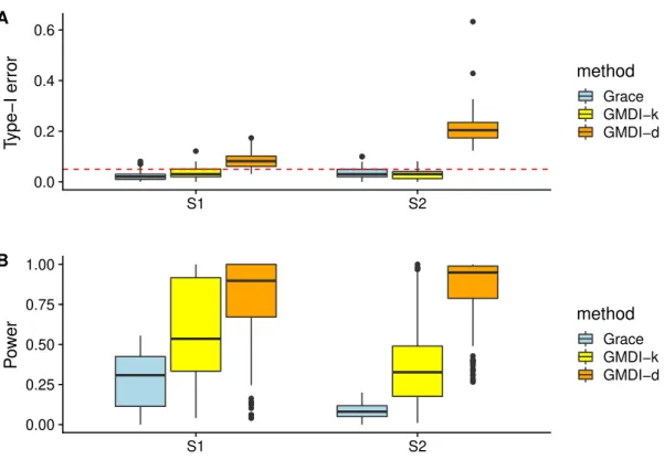
0.0 0.2 0.4 0.6 S1 S2 T ype−I error method Grace GMDI−k GMDI−d A 0.00 0.25 0.50 0.75 1.00 S1 S2 P o w er method Grace GMDI−k GMDI−d B

Figure 3: Boxplots of the type-I error (A) and the power (B) over 500 replications for Setting II withR2 _{“0.6. The S1 and S2 on the x-axis representQ}p1q _andQp2q_{respectively:}

Both GMDI-d and GMDI-k work well under small perturbations of Q, but GMDI-d suffer more than GMDI-k from completely misspecified Q.

difference is that instead of using Q˚_{, we use two perturbed (observed) matrices: Q}p1q

and Qp2q_{. Here, Q}p1q _{is defined similar to Q}˚_{, except that Q}p1q

pi,jq “ 0.1

|i´j| _{for all pi, jq P}

tpa, bq : pa´150qpb´150q ă 0u, and Q_pp2_i,jq_q “ 0.6|i´j| _{for all i, j}

“ 1, . . . ,300. While Qp2q

completely misspecifies the true structure, Qp1q _{roughly captures the structure of Q}˚ _with

some off-diagonal errors, which is a more common scenario in practice.

Only the results of Grace, GMDI-d and GMDI-k for R2 _{“ 0.6 are summarized in Fig.}

3, since other methods are not affected by the perturbation of Q. Comparing Fig. 3 with Fig. 2, it can be seen that when Q suffers from mild perturbations, e.g., Qp1q_{, all three}

methods can still (asymptotically) control the type-I error, but power is compromised in each case due to this misspecifation. WhenQis completely misspecified, e.g.,Qp2q_,

GMDI-d suffers from some inflation of the type-I error, while both Grace anGMDI-d GMDI-k seem to still control the type-I error. However, in other settings, when the observed column structure is completely non-informative, we find that neither method may control the type-I error rate. See the discussions in Section 6 for a robust approach for choosing the appropriate structure among the observed ones.

4.3

Setting III

To assess the effect of sample (row) structure H˚ _{in addition to Q}˚_{, consider}

H˚ pi,jq“ $ ’ ’ ’ ’ ’ ’ ’ ’ & ’ ’ ’ ’ ’ ’ ’ ’ % 1, i“j 0.9|i´j|_{, i} ‰j, iď100, j ď100 0.5|i´j|_{, i} ‰j, ią100, j ą100 0, otherwise.

We simulate X from the matrix-variate model with mean 0, row covariance pH˚_q´1

and column covariance pQ˚

q´1. Finally, using the same β˚ as in Setting I, we simulate the outcome yby

where „ N200p0, σ2pH˚q ´1

q and σ2 is chosen to achieve an R2 of 0.6. We also want to see how perturbations of the row structure would affect the performance of the proposed GMDI procedure. Therefore, we consider the following three scenarios: (S1)H“H˚_{; (S2)} H“Hp1qand (S3)H“I200, whereHp1qis defined similar toH˚except thatH

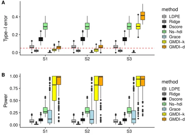
p1q pi,jq“0.1 |i´j| for all pi, jq P tpa, bq:pa´100qpb´100q ă 0u. 0.0 0.2 0.4 S1 S2 S3 T ype−I error method LDPE Ridge Dscore Ns−hdi Grace GMDI−k GMDI−d A 0.00 0.25 0.50 0.75 1.00 S1 S2 S3 P o w er method LDPE Ridge Dscore Ns−hdi Grace GMDI−k GMDI−d B

Figure 4: Boxplots of the type-I error (A) and power (B) over 500 replications for Setting III with R2

“0.6: Both GMDI-d and GMDI-k show robustness with respect to small

per-turbations ofH, but neither can control the type-I error whenHis completely misspecified.

The results are summarized in Fig. 4. Similar to Fig. 2, LDPE, Ridge, Dscore and

hdi all fail to differentiate non-zero coefficients from zero ones. Note that the Dscore test can control the type-I error in Setting I, whereas it fails in this setting with correlated samples. The Grace test performs slightly better thanks to incorporating the column structure, but compared to Fig. 2B, its power is comprised due to ignoring the row structure. For the proposed GMDI, when the pre-specified row structure is correct or mildly perturbed, both GMDI-d and GMDI-k can control the type-I error rate and have considerably higher power than existing methods that can control the type-I error. However, when the samples are mistakenly treated as independent, both GMDI-d and GMDI-k suffer from a large inflation of the type-I error. These results demonstrate the importance of incorporating informative row structures.

5

Analysis of Microbiome Data

In this section, we revisit the microbiome data discussed in Section 1 to illustrate the proposed GMDR and GMDI with real data from Yatsunenko et al. (2012). Recall that the data consists of the counts of p “149 genera sampled from n “100 individuals from the Amazonas of Venezuela, rural Malawi and US metropolitian areas. In the original study, marginal analyses identified a large number of age-associated bacterial species shared in all three populations.

For our analysis, to make the measurements comparable between subjects, we applied the centered log ratio (CLR) transformation to obtain the data matrix X(Gloor and Reid, 2016). As introduced in Section 1, the column structure in X may be characterized by a

pˆpsimilarity kernel derived from the patristic distance between each pair of the tips of the

based on the KEGG ECs in each sample. Specifically, these EC data represent counts of 432 classes of enzymes observed in the bacteria from the same 100 individuals. We also applied the CLR transformation to rows of the EC data and centered its columns to have mean 0. The resulting matrix is denoted by Z, and the row structure is then given by

ntZZTu´1. For ease of presentation, we denote the row and column structure respectively by HM _{and Q}M_{. Similar to Yatsunenko et al. (2012), we are interested in the association}

between bacterial genus and age. As the distribution of age is highly skewed (around 70% of the samples are below 3 years of age), we took the logarithm of age as our outcome, denoted by y.

We first examined the prediction performance of the proposed GMDR estimator com-pared with three existing methods: (i) thelasso estimator (Tibshirani, 1996), (ii) the Ridge estimator (Hoerl and Kennard, 1970) and (iii) the KPR estimator (Randolph et al., 2018). To examine the role that HM _{and Q}M _{play in predicting y, we consider three choices of}

H and Q for both KPR and GMDR; that is, (i) H “ In;Q “ QM, (ii) H “ HM;Q “Ip

and (iii) H“HM_;Q

“QM_{. We denote the KPR (GMDR) estimator corresponding to the}

first, second and third choice by KPR1 (GMDR1), KPR2 (GMDR2) and KPR3 (GMDR3), respectively. These estimators are constructed in the same way as that in Section 4.

Mean squared errors (MSE) for all methods based on leave-one-out cross validation are displayed in Table 1. It can be seen that both KPR1 and GMDR1 yield more accurate prediction results than Ridge, indicating the informativeness of the phylogenetic structure in terms of the prediction accuracy. Similarly, KPR2 and GMDR2 have higher prediction

Table 1: Mean squared errors (MSEs) for different methods.

Method lasso Ridge KPR1 GMDR1 KPR2 GMDR2 KPR3 GMDR3

MSE 0.71 1.13 0.61 0.57 0.78 0.76 0.56 0.52

accuracy than Ridge, indicating that the 100 individuals may exhibit non-trivial correla-tions, which can be reliably characterized by the EC data. Consequently, by incorporating information from both the phylogenetic structure and the EC data, KPR3 and GMDR3 yield the highest prediction accuracy among all the methods. Note that the Ridge esti-mator and all KPR and GMDR estiesti-mators belong to BGMD (5), so these estimators are

all based on GMD components with respect to different two-way structures. Hence, the superior prediction performance of KPR3 and GMDR3 demonstrates the predictive value of the GMD components that incorporate information from HM _{and Q}M_{; this aligns well}

with our observations in Fig. 1. It is also worth noting that every GMDR estimator yields higher prediction accuracy than its corresponding KPR estimator; this may be because of the proposed GCV procedure that guarantees the prediction accuracy of GMDR. As a reference, the prediction accuracy of lasso is higher than KPR2 and GMDR2, but lower than other GMDR and KPR estimators.

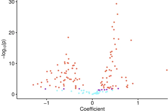
Next, we examined the marginal association between each bacterial genera and age by regressing y on each column of X. Fig. 5 is a volcano plot of the log10-transformed

p-values versus the estimated regression coefficients. Blue dots represent bacteria that are not statistically significant (p ą 0.05); purple dots represent bacteria that are significant (p ď 0.05) but not significant after controlling the false discovery rate (FDR) at 0.1

us-ing the Benjamini–Yekutieli procedure (Benjamini and Yekutieli, 2001); red dots represent bacteria that are still significant after controlling the FDR at 0.1. It can be seen that the majority of bacteria (105 out of 149) are marginally significant after controlling for FDR at 0.1. This is consistent with the results of the marginal Spearman correlations between each bacterial genera and age reported in Yatsunenko et al. (2012). However, since bacteria do not live independently, it is more interesting to examine the association between each

bac-0

10

20

30

−1

0

1

Coefficient

−log

(p)

Figure 5: Marginal analysis: behaviors of the log10-transformed p-values versus the es-timated regression coefficients. Blue dots represent bacteria that are not statistically sig-nificant (p ą 0.05); purple dots represent bacteria that are significant (p ď 0.05) but not significant after controlling the FDR at 0.1; red dots represent bacteria that are still significant after controlling the FDR at 0.1.

terial genera and age while conditioned on all other genera. Two possible explanations for the large number of marginal associations may be that (i) a large number of bacterial gen-era are conditionally associated with age; and (ii) these bacteria are highly correlated but only a few of these are conditionally associated with age. In both situations, existing high-dimensional inferential procedures may fail because either the regression coefficients are

not sparse, or the compatibility condition is no longer satisfied due to the highly correlated variables. However, our GMDI may still work in these situations because of incorporating informative structures. More specifically, given that incorporatingHM _and/orQM_{can lead}

to higher prediction accuracy, we applied the proposed GMDI to all GMDR and KPR esti-mators presented in Table 1. We denote the tests corresponding to KPR1, KPR2, KPR3, GMDR1, GMDR2 and GMDR3 as GMDI-k1, GMDI-k2, GMDI-k3, GMDI-d1, GMDI-d2 and GMDI-d3, respectively. Additionally, we applied the Grace test (Zhao and Shojaie, 2016), Ridge test (B¨uhlmann, 2013) and LDPE (Zhang and Zhang, 2014) for the KPR1, Ridge and lasso estimator, respectively. Genera found significantly associated with age when controlling for FDR at 0.1 are reported in Table 2. While the Ridge test results in no genera associated with the outcome when controlling for FDR at 0.1, the Grace test and LDPE are able to detect 2 and 3 genera, respectively. Notably, when the phylogenetic information is incorporated, considerably more genera are detected: GMDI-d1, GMDI-d3, GMDI-k1 and GMDI-k3, respectively, detect 45, 37, 36 and 32 genera. It can be seen that GMDI-d1 (GMDI-k1) detects more genera than GMDI-d3 (GMDI-k3). This is consistent with the simulation Setting III in Section 4; that is, mistakenly treating correlated samples as independent yields inflated type-I error rates. Also, GMDI-d detects more genera than GMDI-k; this is consistent with the findings in all three simulation settings. One particular bacterium, Lactobacillus, identified by GMDI-d1, GMDI-d3, GMDI-k1 and GMDI-k3, is also discussed in detail in Yatsunenko et al. (2012) as one of the dominant baby gut micro-biota. This may indicate the informativeness of HM _{and Q}M _{for identifying age-associated}

6

Discussions

In this article, we study high-dimensional linear models for two-way structured data in terms of both prediction, estimation and inference. For the purpose of prediction, we ex-tend the classical PCR to GMDR which accounts for arbitrary two-way structures. For estimation and inference of individual regression coefficients, we define a large family of es-timators that include the GMDR estimator and further propose a general high-dimensional inferential framework for any arbitrary estimator in this family, called GMDI. Compared to existing high-dimensional inferential tools, our GMDI can gain more power by allow-ing non-sparse regression coefficients and efficiently incorporatallow-ing the information from the pre-specified two-way structures.

The proposed GMDR and GMDI also provide an approach for integrative analysis of multi-view data; i.e., data collected from multiple sources on the same subjects (Chen et al., 2010; Guo, 2013; Wang et al., 2013). As demonstrated in Section 5, the row structure can be obtained from another data set that collects different features on the same set of samples. Analogously, when there are additional studies addressing the same scientific question, in other words, measuring the same set of variables, one can obtain the column structure from these studies in a similar way.

While the proposed method is motivated and illustrated using microbiome data, our method is generally applicable to arbitrary two-way structured data, such as gene expression data and neuroimaging data. As illustrated in our numerical studies, the proposed GMDI can (asymptotically) control the type-I error rate and have higher power than existing methods even when small perturbations are added to the observed structures, and GMDR can lead to higher prediction accuracy when informative structures are incorporated. In practice, it is often possible to obtain such informative structures in these biological studies.

For example, as illustrated in Section 5, in microbiome studies, a phylogenetic tree is often used to characterize the evolutionary relationship among taxa. For the analysis of gene pression data, one can obtain graph-structured prior information on the genes from, for ex-ample, Kyoto Encyclopedia of Genes and Genomes (KEGG; http://www.genome.jp/kegg) or NCI Pathway Integration Database (NCI graphs; http://pid.nci.nih.gov). For the anal-ysis of neuroimaging data, these structures are often defined as smoothing matrices that are directly related to the structure of the images.

As a robust alternative to fully trusting the observed structures or completely ignoring them, one can combine the observed structures and the identity matrix I through some weight π P r0,1s. Take the column structure Q as an example. For a givenπ P r0,1s, one

can considerQpπq “πQ`p1´πqI. Large value ofπfavors the information inQ, while small value of π protects the analysis being affected by bad choices of Q. This idea, which was also considered in Zhao and Shojaie (2016), can be straightforwardly extended to multiple observed structures, Q1, . . . ,QL, for some L ě 2. Let π “ pπ1, . . . , πLq where πl ě 0 for l “ 1, . . . , L and řL_l“1πl ď 1, and one can consider Qpπq “

řL l“1πlQl` ´ 1´řL_l“1πl ¯ I. In practice, one can find theπ that yields the best prediction accuracy. Such a data-driven Qpπq may be a better approximation to the underlying true column structure than every observed one. Further evaluations of such data adaptive procedures can be a fruitful area of future research.

Appendix

(A1) Derivations of Eq. (6)

We only focus on the high-dimensional case where K “n ăp, noting that similar deriva-tions can be straightforwardly applied to the case where K ą p. It follows from the

definition of βp_KPRpηq that p β_KPRpηq “ `XTHX`ηQ´1˘´1XTHy “QpXTHXQ`ηIpq´1XTHy “QXTH`XQXTH`ηIn ˘´1 y.

Since X“USVT, we get

p β_KPRpηq “ QVSUTH`U`S2`ηIn ˘ UTH˘´1y “QVS´1<sub>S</sub>2 pS2`ηInq´1UTHy. (22)

The last equality in (22) comes from the fact that U is a n ˆn invertible matrix and UT_HU“I

n. DenotingWη “S2pS2 `ηInq´1, we can write

p

β_KPRpηq “QVS´1WηUTHy. (23)

(A2) Proof of Proposition 3.1 and Corollary 3.1

We first recall the definition of βp_jwph_jq in (9) as follows.

p β_jwphjq “ n ÿ i“1 ajiryi´Bp_jph_jq.

Plugging in the definition of Bp_jph_jq, we get

p β_jwphjq “ n ÿ i“1 ajiyri ´ ÿ m‰j ξ_jmw β_minit´hjpξjjw ´1qβjinit “ ÿ m‰j ξ_jmw β_m˚ `ξ<sub>jj</sub>wβ<sub>j</sub>˚´ ÿ m‰j ξ<sub>jm</sub>w β<sub>m</sub>init´hjpξjjw ´1qβ init j `Z w j “ `p1´hjqξjjw `hj ˘ β˚ j ` ÿ m‰j ξ<sub>jm</sub>w pβm˚ ´β init m q` hjpξwjj´1qpβ ˚ j ´β init j q `Z w j , (24) where Zw j “ řn

i“1ajiri. To prove the asymptotic normality of Z

w

j , we first check the

following Lindeberg’s condition; that is,

lim nÑ8 1 s2 n,j n ÿ i“1 E“a2jir 2 i ˆ1t|ajiri| ątsn,ju ‰ “0, for all tą0,

where s2_n,j “σ2řn_i“1a2_ji. Let ε be a random variable distributed like every _ri. Then, 1 s2 n,j n ÿ i“1 E“a2jir 2 i ˆ1t|ajiri| ątsn,ju ‰ “ 1 s2 n,j n ÿ i“1 a2_jiE“ε2ˆ1 |ε| ątsn,j|aji|´1 (‰ ď 1 s2 n,j ˜ _n ÿ i“1 a2_ji ¸ E „ ε2ˆ1 " |ε| ątsn,jt max i“1,...,n|aji|u ´1 * “E « ˆ ε σ ˙2 ˆ1 " | ε σ | ą t řn i“1a 2 ji tmaxi“1,...,n|aji|u´1 *ff . Since lim nÑ8 maxi“1,...,n|aji| řn i“1a2ji “0,

by using the dominated convergence theorem, we get

lim nÑ8 1 s2_n,j n ÿ i“1 E“a2jir 2 i ˆ1t|ajiri| ątsn,ju ‰ “0 for all tą0.

Next, using the Lindeberg central limit theorem, we get s´1

n,jZjw d

Ñ Np0,1q as n Ñ 8. Lastly, we find the explicit form of sn,j by noting

s2_n,j “ σ2 n ÿ i“1 a2_ji “σ2 ´ QVWS´1_UT_L H ` QVWS´1_UT_L H ˘T¯ pj,jq “ σ2 K ÿ l“1 $ & % w2_lσ´2 l ˜ _p ÿ t“1 qjtvtl ¸2, . -;

this completes the proof of Proposition 3.1. Furthermore, it follows from (24) that under

H0,j, ˇ ˇ ˇβp w j phjq ˇ ˇ ˇďmax ˆ max m‰j |ξ w jm|, ˇ ˇh_jpξ_jjw ´1q ˇ ˇ ˙ › ›βinit´β˚ › › 1` ˇ ˇZ_jw ˇ ˇ, 38

which implies Corollary 3.1.

(A3) Proof of Theorem 3.1

We first prove the following concentration result.

Lemma 6.1. Suppose that each column of the design matrix XPRnˆp satisfies}Xj}

2 2 “n

for j “ 1, . . . , p. Further assume that 1, . . . , n are i.i.d. sub-Gaussian random variables

satisfying (7) and have mean 0 and variance σ2. Letting “ p1, . . . , nq, for any δ ą0,

Pr # › ›XT › › 8 nσ ą ˆ Cplogp2pq `δq n ˙1{2+ ďe´δ_,

where the constant C is given in (7).

Proof. First note that for j “1, . . . , p, `XT˘_j “řn_i“1xiji. It follows from (7) that for all t PR, E " exp ˆ txiji σ ˙* ďexp ˆ Cx2 ijt2 2 ˙ ;

this indicates the sub-Gaussianity of σ´1

xiji. By using the Hoeffding inequality

(Wain-wright, 2019) and the assumption that řn_i“1x2

ij “n, we have Pr " |řn_i“1xiji| nσ ąs * ď2 exp " ´ns 2 2C * , for all są0.

Taking a union bound over p choices of j, we get

Pr # › ›XT › › 8 nσ ąs + ď2pexp " ´ns 2 2C * .

Letting δ“ ns 2 2C ´logp2pq, we get Pr # › ›XT › › 8 nσ ą ˆ Cplogp2pq `δq n ˙1{2+ ďe´δ , as claimed.

Recall that Xr “L_HTXD,_ry“ L_HTy and βr ˚

“ DTβ˚. The next lemma characterizes

› › ›∆ ´1{2´ r βpλq ´βr ˚¯› › › 1

, where βrpλq is given in (14) and ∆ is the diagonal matrix whose j-th diagonal element is the j-th eigenvalue of Q.

Lemma 6.2. Suppose that}Q}2 “1and each column of Xr has been scaled so that › › ›Xrj › › › 2 2 “

n for j “1, . . . , p. For any δ ą 0, if λ ě σpn´1pClogp2pq `δqq

1{2

, then under condition (10) and assumptions (A1)–(A3), with probability at least 1´expp´δq, we have

› › ›∆ ´1{2´ r βpλq ´βr ˚¯› › › 1 ď 12s0λ φ2 0,n .

Proof. It follows from the definition of βrpλq that

n´1›› ›ry´Xrβrpλq › › › 2 2 ` 2λ › › ›∆ ´1{2 r βpλq › › › 1 ď n´1›› ›ry´Xrβr ˚› › › 2 2` 2λ › › ›∆ ´1{2 r β˚ › › › 1 .

Then, by the triangle inequality,

n´1›› ›Xrβrpλq ´Xrβr ˚› › › 2 2 ď2n ´1´ r TXr ¯ ´ r βpλq ´βr ˚¯ `2λ ´› › ›∆ ´1{2 r β˚ › › › 1´ › › ›∆ ´1{2 r βpλq › › › 1 ¯ . (25) 40

But from the H¨older’s inequality, n´1´ r T r X ¯ ´ r βpλq ´βr ˚¯ ď › › ›βrpλq ´βr ˚› › › 1 › › ›n ´1 r XT_r › › › 8 . (26) Moreover, since › › ›Xrj › › › 2

2 “n and r satisfies (7), by Lemma 6.1, for any δą0,

Pr # › › ›n ´1 r XTr › › › 8 ą σ ˆ Cplogp2pq `δq n ˙1{2+ ďe´δ_{. (27)}

Combining (25), (26) and (27), for any δą0,

n´1›› ›Xrβrpλq ´Xrβr ˚› › › 2 2 ď 2σ ˆ Cplogp2pq `δq n ˙1{2<sub>›</sub> › ›βrpλq ´βr ˚› › › 1` 2λ ´› › ›∆ ´1{2 r β˚ › › › 1´ › › ›∆ ´1{2 r βpλq › › › 1 ¯

with probability at least 1´expp´δq. Since}Q}2 “1, it can be seen that

› › ›βrpλq ´βr ˚› › › 1 ď › › ›∆ ´1{2´ r βpλq ´βr ˚¯› › › 1 .

Thus, choosing λěσpn´1pClogp2pq `δqq

1{2 , we get n´1›› ›Xrβrpλq ´Xrβr ˚› › › 2 2 ď λ › › ›∆ ´1{2´ r βpλq ´βr ˚¯› › › 1`2λ ´› › ›∆ ´1{2 r β˚ › › › 1´ › › ›∆ ´1{2 r βpλq › › › 1 ¯ ď λ › › › ´ ∆´1{2 r βpλq ¯ S˚ ´ ´ ∆´1{2 r β˚ ¯ S˚ › › › 1` λ › › › › ´ ∆´1{2 r βpλq ¯ ´S˚ › › › › 1 ` 2λ " › › › ´ ∆´1{2 r βpλq ¯ S˚ ´ ´ ∆´1{2 r β˚ ¯ S˚ › › › 1´ › › › › ´ ∆´1{2 r βpλq ¯ ´S˚ › › › › 1 * “3λ › › › ´ ∆´1{2 r βpλq ¯ S˚ ´ ´ ∆´1{2 r β˚ ¯ S˚ › › › 1´ λ › › › › ´ ∆´1{2 r βpλq ¯ ´S˚ › › › › 1 .

Then, since › › ›Xrβrpλq ´Xrβr ˚› › › 2 2 ě 0, we have 3 › › › ´ ∆´1{2 r βpλq ¯ S˚´ ´ ∆´1{2 r β˚ ¯ S˚ › › › 1 ě › › › › ´ ∆´1{2 r βpλq ¯ ´S˚ › › › › 1 . (28)

Then, by Assumption (A3), we get

φ2 0,n s0 › › › ´ ∆´1{2 r βpλq ¯ S˚ ´ ´ ∆´1{2 r β˚ ¯ S˚ › › › 2 1 ď 3λ › › › ´ ∆´1{2 r βpλq ¯ S˚ ´ ´ ∆´1{2 r β˚ ¯ S˚ › › › 1 .

Also, note that

› › ›∆ ´1{2´ r βpλq ´βr ˚¯› › › 1 “ › › › ´ ∆´1{2 r βpλq ¯ S˚´ ´ ∆´1{2 r β˚ ¯ S˚ › › › 1` › › › › ´ ∆´1{2 r βpλq ¯ ´S˚ › › › › 1 Thus, (28) yields › › ›∆ ´1{2´ r βpλq ´βr ˚¯› › › 1 ď 4 › › › ´ ∆´1{2 r βpλq ¯ S˚ ´ ´ ∆´1{2 r β˚ ¯ S˚ › › › 1 , and we get › › ›∆ ´1{2´ r βpλq ´βr ˚¯› › › 1 ď 12s0λ φ2 0,n ,

for any λěσpn´1pClogp2pq `δqq

1{2

.

Now we use Lemma 6.2 to prove Theorem 3.1. For any κ ą C, we take δ “ pκ´

Cqlogp2pq in Lemma 6.2 to obtain

› › ›∆ ´1{2´ r β˚´βrpλq ¯› › › 1 “ σop #˜c logp n ¸r+ . (29) 42

Thus, it can be seen that |ζjphjq| “ ˇ ˇ ˇ ˇ ˇ p ÿ m“1 ξ_jmw pβ˚ m´β init m q ´ ` p1´hjqξjjw `hj ˘ pβ˚ j ´β init j q ˇ ˇ ˇ ˇ ˇ “ ˇ ˇ ˇ “` QVWVT ´ p1´hjqΞ´hjIp ˘ pβ˚ ´βinitq‰<sub>j</sub> ˇ ˇ ˇ ď › › › › ” ` QVWVT ´ p1´hjqΞ´hjIp ˘ D∆1{2ı pj,¨q › › › › 8 › › ›∆ ´1{2´ r β˚´βrpλq ¯› › › 1. (30)

Combining (29) and (30), it can be seen that

lim nÑ8Pr # |ζjphjq| ďσ › › › › ” ` QVWVT ´ p1´hjqΞ´hjIp ˘ D∆1{2ı pj,¨q › › › › 8 ˜c logp n ¸r+ “1.

Finally, (15) directly follows from Proposition 3.1.

(A4) Proof of Theorem 3.2

We first note that P_jwphjq ď α is equivalent to

ˇ ˇ ˇβp w j phjq ˇ ˇ ˇěΨjphjq `qp1´α{2q b σ2 Ωwjj. Since ˇ ˇ ˇβp w j phjq ˇ ˇ ˇ“ ˇ ˇ ` p1´hjqξjjw `hjq ˘ β˚ j `ζjphjq `Zjw ˇ ˇ, we know Pr !ˇ ˇ ˇβp w j phjq ˇ ˇ ˇěΨjphjq `qp1´α{2q b σ2 Ωwjj ) ě Pr ! |`p1´hjqξjjw `hjq ˘ β˚ j| ´ |ζjphjq| ´ |Zjw| ěΨjphjq `qp1´α{2q b σ2 Ωwjj ) .

Hence, it suffices to show Pr ! |`p1´hjqξjjw `hjq ˘ β˚ j| ´ |ζjphjq| ´ |Zjw| ěΨjphjq `qp1´α{2q b σ2 Ωwjj ) ěψ. (31)

It follows from Proposition 3.1 that as n Ñ 8, pσ2Ωw_jjq´1{2Z_jw Ñd Np0,1q. Thus, for

ψ P p0,1q, if |`p1´hjqξwjj`hjq ˘ β˚ j| ´ |ζjphjq| ´Ψjphjq ´qp1´α{2q a σ2 Ωwjj a σ2 Ωwjj ěqp1´ψ{2q, (32)

then (31) holds. Noting that limnÑ8Prp|ζjphjq| ďΨjq “1, we know that as n Ñ 8, (32)

holds if ˇ ˇβ_j˚ ˇ ˇě |p1´h_jqξ_jjw `h<sub>j</sub>|´1¨ ´ 2Ψjphjq ` ` qp1´α{2q`qp1´ψ{2q ˘b σ2 Ωwjj ¯ ;

this completes of proof of Theorem 3.2.

References

Allen, G. I., L. Grosenick, and J. Taylor (2014). A generalized least-square matrix decom-position. Journal of the American Statistical Association 109(505), 145–159.

Benjamini, Y. and D. Yekutieli (2001). The control of the false discovery rate in multiple testing under dependency. The Annals of Statistics 29(4), 1165–1188.

Besse, P. and J. O. Ramsay (1986). Principal components analysis of sampled functions. Psychometrika 51(2), 285–311.

Boente, G. and R. Fraiman (2000). Kernel-based functional principal components.Statistics Probability Letters 48(4), 335 – 345.

B¨uhlmann, P. (2013). Statistical significance in high-dimensional linear models. Bernoulli 19(4), 1212–1242.

Cai, T. and P. Hall (2006). Prediction in functional linear regression. The Annals of Statistics 34, 2159–2179.

Chen, N., J. Zhu, and E. P. Xing (2010). Predictive subspace learning for multi-view data: a large margin approach. InAdvances in Neural Information Processing Systems 23, pp. 361–369. Curran Associates, Inc.

Chernozhukov, V., C. Hansen, and M. Spindler (2015). Valid selection and post-regularization inference: An elementary, general approach. Annual Review of Eco-nomics 7(1), 649–688.

Cook, R. D. (2007). Fisher lecture: Dimension reduction in regression. Statistical Sci-ence 22(1), 1–26.

Escoufier, Y. (1987). The duality diagram: a means for better practical applications. In Develoments in Numerical Ecology, pp. 139–156. Springer.

Gloor, G. B. and G. Reid (2016). Compositional analysis: a valid approach to analyze microbiome high-throughput sequencing data. Canadian journal of microbiology 62(8), 692–703.

Guo, Y. (2013). Convex subspace representation learning from multi-view data. In Twenty-Seventh AAAI Conference on Artificial Intelligence.