Computing Label-Constraint Reachability in Graph
Databases
Ruoming Jin
1Hui Hong
1Haixun Wang
2Ning Ruan
1Yang Xiang
11
Kent State University, Kent, OH 44242
{jin, hhong, nruan, yxiang}@cs.kent.edu
2
Microsoft Research Asia
[email protected]
ABSTRACT
A huge amount of graph data (biological networks, semantic web, ontologies, social networks) is being generated. Many of these real-world graphs are edge-labeled graphs, i.e., each edge is associated with a label that denotes the relationship between the two vertices connected by the edge. Given this, a fundamental research problem on the labeled graphs is how to handle the label-constraint reachability query: Can vertexureach vertexvthrough a path whose edge labels are constrained by a set of labels? In this work, we formally introduce the labeled reachability query problem, and pro-vide two initial algorithms that categorize its computational complexity. We then generalize the transitive closure for the labeled graph, and introduce a new index framework which utilizes a directed spanning tree to compress the generalized transitive closure. We optimize the index for minimal mem-ory cost and we propose methods which utilize the directed maximal weighted spanning tree algorithm and sampling techniques to maximally compress the generalized transi-tive closure. After establishing an interesting link between the reachability problem and the geometric search problem, we utilize the geometric search structures, such as multidi-mensional kd-trees or the range-search trees, to enable fast query processing. In our extensive experimental evaluation on both real and synthetic datasets, we find our tree-based index can significantly reduce the memory cost of the gener-alized transitive closure while still being able to answer the query very efficiently.
Categories and Subject Descriptors
H.2.8 [Database management]: Database Applications— graph indexing and querying
General Terms
PerformanceKeywords
Graph indexing, Reachability queries, Transitive closure, Maximal directed spanning tree, Sampling
1.
INTRODUCTION
A huge amount of graph data (biological networks, se-mantic webs, social networks) is being generated. How to manage these large graphs in a database system has become an important research issue in the database research com-munity. One of the most fundamental research problems is
the reachability query, which asks if one vertex can reach another or not. This is a seemingly simple but very difficult problem due to the sheer size of these large graphs. In re-cent years, a number of algorithms have been proposed to handle graph reachability queries [16, 2, 27, 7, 26, 17, 8].
However, many real-world graphs are edge-labeled graphs, i.e., edges are associated with labels to denote different types of relationships between vertices. The reachability query for labeled graphs often involves constraints on the path con-necting two vertices. Here, we list several such applications:
Social Networks:
.
In a social network, each person is rep-resented as a vertex and two persons are linked by an edge if they are related. The relationships between two persons are represented through different types of labels. For instance, such relationships may includeparent-of,student-of, brother-of,sister-of, friend-of,employee-of, consultant-of, follower-of, etc. Many queries in social networks seek to discover how one personArelates to another personB. These queries in general can be written as if there is a path from A to Bwhere the labels of all edges in the path are either a specific type or belong to a specified set of labels. For instance, if we want to know whetherAis a remote relative ofB, then we ask if there is a path from A toB where each edge la-bel along the path is one of parent-of, child-of,brother-of, sister-of.
Bioinformatics:
.
Understanding how metabolic chain re-actions take place in cellular systems is one of the most fun-damental questions in system biology. To answer these ques-tions, biologists utilize so-called metabolic networks, where each vertex represents a compound, and a directed edge be-tween two compounds indicates that one compound can be transformed into another one through a certain chemical re-action. The edge label records the enzymes which control the reaction. One of the basic questions is whether there is a certain pathway between two compounds which can be active or not under certain conditions. The condition can be described as the availability of a set of enzymes. Here, again, our problem can be described as a reachability query with certain constraints on the labels of the edges along the path.To summarize, these queries ask the following question: Can vertexureach vertexvthrough a path whose edge labels must satisfy certain constraints? Typically, the constraint is membership: the path’s edge labels must be in the set of constraint labels. Alternatively, we can ask for a path which avoids any of these labels. These two forms are equivalent.
We note that this type of query can also find applications in recommendation search in viral marketing [20] and reacha-bility computation in RDF graphs, such as Wikipedia and YAGO [25].
The constraint reachability problem is much more com-plicated than the traditional reachability query which does not consider any constraints. Existing work on graph reach-ability typically constructs a compact index of the graph’s transitive closure matrix. The transitive closure can be used to answer the Yes/No question of reachability, but it cannot tell how the connection is made between any two vertices. Since the index does not include the labeling information, it cannot be expanded easily to answer our aforementioned label-constraint reachability query.
The constraint reachability problem is closely related to the simple path query and the regular expression path query for XML documents and graphs. Typically, these queries describe the desired path as a regular expression and then search the graph to see if such a path exists or not. An XPath query is a simple iteration of alternatingaxes(/and
//) and tags (or labels), and it can be generalized by us-ing regular expressions to describe the paths between two or a sequence of vertices [1]. We can look at our constraint reachability query as a special case of theregular simple path query. However, the general problem of finding regular sim-ple paths has proven to be NP-comsim-plete [21]. The existing methods to handle such queries are based on equivalence classes and refinement to build compact indices and then match the path expression over such indices [22, 12]. On the other hand, a linear algorithm exists for the constraint reachability problem. Thus, the existing work on quering XML and graphs cannot provide an efficient solution to our constraint reachability query.
1.1
Our Contributions
In this work, we provide a detailed study of the constraint reachability problem and offer an efficient solution. We be-gin by investigating two simple solutions, representing two extremes in the spectrum of solutions. First, we present an online search (DFS/BFS) algorithm. This method has very low cost for index construction and minimal index size. However, online search can be expensive for very large graphs. Second, we consider precomputing the necessary path infor-mation (of labels) between any two vertices. This is similar to building the transitive closure for answering the tradi-tional reachability query. This approach can answer the con-straint reachability query much faster than the first method since we can use the precomputed table to answer queries without traversing the graph. However, the size of the pre-computed path-label sets is much larger than that of the traditional transitive closure for reachability query. In sum-mary, the first approach uses the least amount of memory but has high computational cost for query answering, while the second approach answers the query efficiently, but uses a large amount of memory.
The major research problem here is how to find a (good) compromise between these two approaches. Specifically, we would like to significantly reduce the memory cost of the fully precomputed table and still be able to answer the reach-ability query efficiently. In this work, we propose a novel tree-based index frameworkfor this purpose. Conceptually, we decompose any path into three fragments: beginning, end, and middle fragments. Its beginning and end parts
al-ways come from a spanning tree structure, and its middle fragment will be precomputed by a partial transitive clo-sure. We will not fully materialize the transitive closure, but only record a small portion of it, which we refer to as thepartial transitive closure. Interestingly, we find that the problem of minimizing the size of the partial transitive clo-sure can be effectively transformed into amaximal directed spanning tree problem. We also devise a query processing scheme which will effectively utilize multi-dimensional ge-ometric search structures, such as kd-tree or range search tree, to enable fast query processing.
Our main contributions are as follows:
1. We introduce the label-constraint reachability (LCR) problem, provide two algorithms to categorize its com-putational complexity and generalize the transitive clo-sure (Section 2).
2. We introduce a new index framework which utilizes a directed spanning tree to compress the generalized transitive closure (Section 3).
3. We study the problem of constructing the index with minimal memory cost and propose methods which uti-lize the directed maximal weighted spanning tree algo-rithm and sampling techniques to maximally compress the generalized transitive closure (Section 4).
4. We present a fast query processing approach for LCR queries. Our approach is built upon an interesting link between the reachability search problem and geomet-ric search problem, permitting us to utilize geometgeomet-ric search structures, such as multidimensional kd-trees or range search tree for LCR queries (Section 5). 5. We conducted a detailed experimental evaluation on
both real and synthetic datasets. We found our tree-based index can significantly reduce the memory cost of the generalized transitive closure while still being able to answer the query very efficiently (Section 6).
2.
PROBLEM STATEMENT
A database graph (db-graph) is a labeled directed graph
G= (V, E,Σ, λ), whereV is the set of vertices,Eis the set
of edges, Σ is the set of edge labels, andλis the function that assigns each edgee∈Ea labelλ(e)∈Σ. A pathpfrom ver-texutovin a db-graphGcan be described as a vertex-edge alternating sequence, i.e.,p= (u, e1, v1,· · ·, vi−1, ei, vi,· · ·, en, v). When no confusion will arise, we use only the vertex se-quence to describe the pathpfor simplicity, i.e.,p= (v0, v1,· · ·, vn). We usepath-labelL(p) to denote the set of all edge labels in the pathp, i.e.,L(p) ={λ(e1)} ∪ {λ(e2)} ∪ · · · ∪ {λ(en)}.
Definition 1. (Label-Constraint Reachability) Given two vertices,uandvin db-graphG, and a label setA, where
u, v ∈V and A⊆Σ, if there is a path p from vertex uto
v whose path-label L(p) is a subset of A, i.e., L(p) ⊆ A, then we say ucan reach v with label-constraintA, denoted as (u−→A v), or simply v is A-reachable fromu. We also refer to pathpas anA-pathfromutov. Given two vertices
u andv, and a label setA, thelabel-constraint reacha-bility (LCR) queryasks ifvisA-reachable fromu.
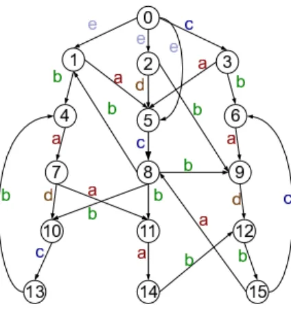
Figure 1: Running Example
Figure 2: (0,9)Path-Label
Throughout this paper, we will use Figure 1 as a running example, using integers to represent vertices and letters to represent edge labels. In this example, we can see that ver-tex 0 can reach verver-tex 9 with the label-constraint{a, b, c}. In other words vertex 9 is{a, b, c}-reachable from vertex 0. Furthermore, the path (0,3,6,9) is a{a, b, c}-path from ver-tex 0 to 9.
In the following, we will discuss two basic approaches for answering the label-constraint reachability (LCR) queries.
2.1
Online DFS/BFS Search
The most straight-forward method for answering an LCR query is online search. We can apply either DFS (depth-first search) or BFS (breadth-(depth-first search), together with the label-constraint, to reduce the search space. Let us consider the DFS for theA-reachable query from vertex utov. For simplicity, we say that a vertexxisA-adjacentto vertexu, if there is an edgeelinkingutox, i.e.,e= (u, x) and the edge label ofeis contained inA,λ(e)∈A. Starting from vertex
u, we recursively visit allA-adjacent vertices until we either reach vertexv or have searched all the reachable vertices fromuwithout reachingv. Clearly, inO(|V|+|E|), we can concludev is A-reachable from u or not. Thus, answering the label-constraint reachability query can be done in poly-nomial time. However, since the size of the db-graph is very large (it can easily contain millions of vertices), such simple
online search is not acceptable for fast query answering in a graph database.
We may speedup such online search by a more “focused” search procedure. The speedup is based on the observation that in the above procedure, we may visit a lot of vertices from vertexuwhich cannot reach vertexvno matter what path we take. To avoid this, we can utilize the existing work on the reachability query [16, 2, 27, 7, 26, 17, 8], which tells whether one vertex can reach another vertex very quickly. Thus, when we try to visit a new vertex from the current vertex, denoted asu′, we require this vertex is not onlyA
-adjacent to u′, but also can reach the destination vertexv
(utilizing the traditional reachability index). Note that the BFS procedure can be extended in a similar manner.
2.2
Generalized Transitive Closure
An alternative approach is to precompute thepath-label set, i.e., all path-labels between any two vertices. Note that this corresponds to the transitive closure for the reachabil-ity query. The major difficulty for the path-label sets is the space cost. The upper bound for the number of all path-labels between any two vertices is 2|Σ|. Thus, the total
stor-age complexity isO(|V|22|Σ|), which is too expensive.
However, to answer the label-constraint reachability (LCR) query, we typically only need to record a small set of path-labels. The intuition is that if vertex u can reach vertex
v with label constraintA, thenucan reachv with any la-bel constraintA′⊇A. In other words, we can always drop
the path-labels fromu tovwhich are supersets of another path-label from uto vwithout affecting the correctness of the LCR query result. For instance, in our running example from vertex 0 to 9, we have one path (0,2,9), which has the path-label{b, d}, and another path (0,2,5,8,9), which has the path-label{b, d, e, a}. Then, for any label-constraintA, we will not need to check the second path to answer the query.
To formally introduce such a reduction, we need to con-sider what set of path-labels are sufficient for answering LCR query.
Definition 2. (Sufficient Path-Label Set) Let S be a set of path-labels from vertex u to v. Then, we say S
is a sufficient path-label set if for any label-constraint A,
u−→A v, the LCR query returns true if and only if there is a path-labels∈S, such thats⊆A.
Clearly the set of ALL path-labels from vertex u to v, denoted asS0, is sufficient. Our problem is how to find the minimal sufficient path-label set, which contains the smallest number of path-labels. This set can be precisely described in Theorem 1.
Theorem 1. LetS0 be the set of all path-labels from ver-texutov. The minimal sufficient path-label set fromutov, referred to asSmin is unique and includes only those path-labels which do not have any (strict) subsets inS0, i.e.,
Smin={L(p)|L(p)∈S0 ∧∄L(p′)∈S0, such that,L(p′)⊂L(p)} In other words, for any two path-labels, s1 and s2 in Smin, we haves16⊂s2 ands26⊂s1.
This theorem clearly suggests that we can remove all path-label sets in S which contain another path-label set in S
is omitted for simplicity. In addition, we can also utilize the partially order set (poset) to describe the minimal suffi-cient path-label set. Let the subset (⊆) relationship be the binary relationship “≤” over S0, i.e., L1 ≤ L2 iffL1 ⊆L2 (L1,L2 ∈S0). Then, the minimal sufficient path-label set is the lower bound of S0 and consists all and only mini-mal elements[3]. Figure 2 shows the set of all path-labels from vertex 0 to 9 using a Hasse Diagram. We see that its minimal sufficient path-label set contains only two elements:
{b, e}and{a, b, c}. The upper bound for the cardinality of
any minimal sufficient path-label set is ` |Σ| ⌊|Σ|/2⌋
´
. This is also equivalent to the maximal number of non-comparable elements in the power set of Σ. The bound can be easily ob-served and in combinatorics is often referred to as Sperner’s Theorem [3].
Algorithm Description: We present an efficient algo-rithm to construct the minimal sufficient path-label set for all pairs of vertices in a given graph using a dynamic pro-gramming approach corresponding to a generalization of Floyd-Warshall algorithm for shortest path and transitive closure [10]).
LetMk(u, v) denote the minimal sufficient path-label set of those paths fromutovwhose intermediate vertices are in {v1,· · ·,vk}. Now we consider how to compute the minimal sufficient path-label sets of the paths from each vertexutov
with intermediate vertices up tovk+1, i.e.,Mk+1(u, v). Note thatMk+1(u, v) describe two types of paths, the first type is those paths using only intermediate vertices (v1,· · ·, vk) and the second type is those paths going through the inter-mediate vertices up tovk+1. In other words, the second type of paths can be described as a path composed of two frag-ments, first fromutok+ 1 and then fromk+ 1 toj. Given this, we can compute the minimal sufficient path-label sets using these two types of paths recursively by the following formula: Mk+1(u, v) = P rune(Mk(u, v)∪(Mk(u, k)⊙Mk(k, v))); M0(u, v) = λ((u, v)) if (u, v)∈E ∅ if (u, v)∈/E
Here,Pruneis the function which simply drops all the path-labels which are the supersets of other path-path-labels in the input set. In other words,Prunewill produce the lower bound of the input path-label set. The⊙operatorjoins two sets of sets, such as{s1, s2}⊙{s1′, s′2, s′3}={s1∪s′1, s1∪s′2,· · ·, s2∪
s′
3}, wheresiands′jare sets of labels. Besides, we can easily observe that
P rune(S1∪S2) =P rune(P rune(S1)∪P rune(S2))
P rune(S1⊙S2) =P rune(P rune(S1)⊙P rune(S2)) whereS1 and S2 are two path-label sets. The correctness of the recursive formula for theMk+1(u, v) naturally follows these two equations.
Algorithm 1 sketches the dynamic programming proce-dure which constructs the minimal sufficient path-label sets for all pairs of vertices in a graphG. The worst case com-putational complexity isO(|V|32|Σ|) for this dynamic pro-cedure and its memory complexity isO(|V|2` |Σ|
⌊|Σ|/2⌋
´ ).
3.
A TREE-BASED INDEX FRAMEWORK
The two methods we described in Section 1, online search and generalized transitive closure computation, represent two extremes for label-constraint reachability (LCR) query processing: the first method has the least memory cost for
Algorithm 1LabeledTransitiveClosure(G(V, E,Σ, λ))
Parameter: G(V, E,Σ, λ) is a Database Graph
1: for each(u, v)∈V ×V do 2: if(u, v)∈Ethen 3: M[u, v]← {λ((u, v))} 4: else 5: M[u, v]← ∅ 6: end if 7: end for 8: fork= 1 to|V|do 9: for each(u, v)∈V ×V do 10: M[u, v]←Prune(M[u, v]∪(M[u, k]⊙M[k, v])) 11: end for 12: end for
indexing but very high computational cost for answering the query, while the second method has very high memory cost for indexing but has low computational cost to answer the query. Thus, the major research question we address in the present work is how to devise an indexing mechanism which has a low memory cost but still can process LCR queries efficiently.
The basic idea of our approach is to utilize a spanning tree to compress the generalized transitive closure which records the minimal sufficient path-label sets between any pair of vertices in the db-graph. Though spanning trees have been applied to directed acyclic graphs (DAG) for com-pressing the traditional transitive closure [2], our problem is very different and much more challenging. First, both db-graphs and LCR queries include edge labels which cannot be handled by traditional reachability index. Second, the db-graph in our problem is a directed db-graph, not a DAG. We cannot transform a directed graph into a DAG by coalesc-ing the strongly connected components into a scoalesc-ingle vertex since much more path-label information is expressed in these components. Finally, the complexity arising from the label combination, i.e, the path-label sets, is orders of magnitude higher than the basic reachability between any two vertices. Coping with such complexity is very challenging.
To deal with these issues, our index framework includes two important parts: a spanning tree (or forest) of the db-graph, denoted as T, and a partial transitive closure, de-noted as N T, for answering the LCR query. At the high level, the combination of these two parts contains enough information to recover the complete generalized transitive closure. However, the total index size required by these two parts is much smaller than the complete generalized transi-tive closure. Furthermore, LCR query processing, which in-volves a traversal of the spanning tree structure and search-ing over the partial transitive closure, can be carried out very efficiently.
Let G(V, E,Σ, λ) be a db-graph. LetT(V, ET,Σ, λ) be
a directed spanning tree (forest) of the db-graph, where
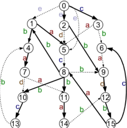
ET ⊆ E. Note that we may not be able to find a span-ning tree, instead, we may find a spanspan-ning forest. In this case, we can always construct a spanning tree by creating a virtual root to connect the roots of the trees in the spanning forest. Therefore, we will not distinguish spanning tree and spanning forests. For simplicity, we always assume there is a virtual root. For convenience, we say an edgee ∈ET is a tree edge and an edge inE but not in ET is a non-tree edge. There are many possible spanning trees for G. Fig-ure 3 shows one spanning tree for our running example graph
Figure 3: Spanning Tree and Non-Tree Edges
Figure 4: Partial Transitive Closure (NT) (S. for Source and T. for Target)
(Figure 1), where the bold lines highlight the edges in the spanning tree, and the dotted lines are the non-tree edges in the graph.
To utilize the spanning tree structureT of the db-graph
Gfor compressing the generalized transitive closure, we for-mally introduce a classification of paths between any two nodes.
Definition 3. (Path Classification)Consider a db-graph
Gand its spanning treeT. For a pathp= (v0, e1, v1,· · ·, en, vn) inG, we classify it into three types based on its starting edge (e1) and ending edge (en):
1. (Ps)contains all the paths whose starting edge is a tree-edge, i.e.,e1∈ET;
2. (Pe)contains all the paths whose last edge is a tree-edge, i.e.,en∈ET;
3. (Pn)contains all the paths whose starting edge and end edge are both non-tree edges, i.e.,e1, en∈E\ET.
We also refer the third type path Pn asnon-tree path. In addition, if all the edges in path p are tree-edges, i.e.,
ei ∈ ET for 1≤i≤n, then, we refer to it as anin-tree
path.
Note that a path (if it starts with a tree-edge and ends
with a tree-edge) can belong to both the first and the second types of paths. Indeed, the in-tree path is such an example, and it is a special case of both Ps and Pe paths. In our running example (Figure 3), path (0,2,9,12) is an in-tree path from vertex 0 to 12, path (0,2,5,8,11,14,12) is an example of Ps, path (0,5,8,11,14,12) is a non-tree path
Pn, and path (0,5,8,9,12) is an example of the second path typePe.
Now, we further introduce the classification of path-label sets and especially thepartial transitive closure, which car-ries the essential non-tree path labels.
Definition 4. (Partial Transitive Closure)LetM(u, v) be the minimal sufficient path-label set from vertexutovin
G. Letpbe a path from vertex utov. Then we define the three subsets ofM(u, v)based on the path types:
1. Ms(u, v) ={L(p)|p∈Ps} ∩M(u, v);
2. Me(u, v) ={L(p)|p∈Pe} ∩M(u, v);
3. N T(u, v) ={L(p)|p∈Pn}∩M(u, v)−Ms(u, v)−Me(u, v); Thepartial transitive closureN T records all theN T(u, v), (u, v)∈V ×V, whereN T(u, v)6=∅.
Clearly, the union of these three subsets is the minimal sufficient path-label set fromutov, i.e.,M(u, v) =Ms(u, v)∪
Me(u, v)∪N T(u, v). Further,Ms(u, v)∩Me(u, v) may not be empty, but (Ms(u, v)∪Me(u, v))∩N T(u, v) =∅. Theo-rem 2 below states that we only need to record the partial transitive closure (N T) in combination with the spanning tree T in order to recover the complete transitive closure
M. Thus, it lays the theoretical foundation of our indexing framework: T and N T together record sufficient informa-tion for LCR query processing. Figure 4 shows theN T for the spanning tree (Figure 3) in our running example. Here, the N T has only a total of 26 entries, i.e., the number of (u, v) which is not empty,N T(u, v)6=∅, and the cardinality of each entry (the number of path-labels) is one. Among these non-empty entries, 12 of them are simply the edges in the original graph. Thus, only extra 14 entries are needed to record in N T to recover the full transitive closure M. Note that our running example graph has a total of 16 ver-tices and 29 edges, and the size of M is 210, P
(u,v)∈V×V |M(u, v)|= 210.
Theorem 2. (Reconstruction Theorem: T+NT→
M(u,v))Given a db-graphGand a spanning treeTofG, let
N T be the partial transitive closure defined in Definition 4. Let Succ(u) be all the successors of u in the tree T. Let
P red(v)be all the predecessors of v in treeT. In addition,
u′ ∈ Succ(u) and v′ ∈ P red(v). Then, we can construct
M′(u, v) of path-label sets fromutov usingT andN T as follows:
M′(u, v) = {{L(PT(u, u′))} ⊙N T(u′, v′)⊙ {L(PT(v′, v))}|
u′∈Succ(u)andv′∈P red(v)}
where, for any vertexx,L(PT(x, x)) =L(PN(x, x)) =∅and
N T(x, x) = {∅}. Then we have, for any vertices u andv,
M(u, v)⊆M′(u, v), andM(u, v) =P rune(M′(u, v)).
Proof Sketch:
To prove this theorem, we will establish the following three-segment path decomposition scheme for any path p
from a vertexuto another vertexv, i.e.,p= (v0, e1, v1,· · ·, en, vn), where u=v0 andv=vn. Leteibe the first non-tree edge andejbe the last non-tree edge in pathp(i≤j). Letu′ be
the beginning vertex of the first non-tree edgeei,u′=vi−1 andv′be the end vertex of the last non-tree edgeej,v′=vj.
Now, we can decompose path p into three segments: 1) the starting in-tree path fromutou′, denoted as PT(u, u′); 2) the intermediate non-tree path fromu′ tov′, denoted as PN(u′, v′); 3) the ending in-tree path fromv′ to v denoted asPT(v′, v). Note that certain segments can be empty and we definethe empty segmentasPN(x, x) =PT(x, x) for any vertexx.
Given this, let us consider such decomposition for each type of path fromutov.
Case 1: If there is anin-tree path pfromuto v, then we can directly represent it as
L(p) =L(PT(u, v)) =L(PT(u, u′))∪ ∅ ∪L(PT(u′, v)) whereu′∈ {v
1,· · ·, vn}andu′∈Succ(u) andu′∈P red(v) sincepis an in-tree path.
Case 2:Ifp∈(Ps∪Pe)\PT(u, v) (pathpis aPsorPepath but not an in-tree path), then, there is at least onenon-tree edgeinp. Thus, we can findu′ andv′ in pathp, such that
u′∈Succ(u),v′∈P red(v) and thesubpath ofpfromu′ to
v′is anon-tree path. Then, ifL(p)∈M(u, v), we have
L(p)∈ {L(PT(u, u′))} ⊙N T(u′, v′)⊙ {L(PT(v′, u))}
Case 3: Ifp∈Pn (a non-tree path), then, similar analysis asCase2 holds.
Putting these together, we have
M(u, v) = P rune({{L(PT(u, u′))} ⊙N T(u′, v′)⊙ {L(PT(v′, v))}|
u′∈Succ(u) andv′∈P red(v)})
2
To apply this theorem for index construction and LCR query processing, we need to address the following two key research questions: 1) Different spanning treesT can have very differently sized partially transitive closuresN T. How can we find an optimal spanning tree T to minimize the total index size, and specifically, the cost of partial transi-tive closureN T? 2) How can we utilize the spanning tree
T and partial transitive closure N T to efficiently answer the LCR query? This is not a trivial question and a good query processing scheme can be as fast as we directly query the complete generalized transitive closure but with a much smaller memory cost. We will study the first question (opti-mal index construction) in Section 4 and the second question (efficient LCR query processing) in Section 5.
4.
OPTIMAL INDEX CONSTRUCTION
In this section, we study how to construct an optimal spanning tree T to minimize the cost of partial transitive closureN T, which is the dominant cost of our entire index framework. In Subsection 4.1, we will introduce an inter-esting approach based on themaximally directed spanning tree algorithm [9, 11] to tackle this problem. However, this solution relies on the fully materialization of general-ized transitive closureM. Though this can be done using the LabeledTransitiveClosurealgorithm (Algorithm 1 in Subsec-tion 2.2), it becomes very expensive (for both computaSubsec-tion and storage) when the size of the graph becomes large. In Subsection 4.2, we present a novel approximate algorithm which can find with high probability a spanning tree with bounded cost difference compared with the exact maximal spanning tree.
4.1
Directed Maximal Spanning Tree for
Gen-eralized Transitive Closure Compression
LetMbe the generalized transitive closure which contains the minimal sufficient path-label set between any two ver-ticesuandv. Recall that for a spanning treeT,N T(u, v) =M(u, v)−Ms(u, v)−Me(u, v) records the “essential” path-labels of non-tree paths which cannot be replaced by either an type Ps path (beginning with a tree-edge) or Pe path (ending with a tree-edge). Given this, the size of the partial transitive closureN T can be formally defined as
cost(N T) = X
(u,v)∈V×V
|N T(u, v)|.
However, the direct minimization ofcost(N T) is hard and the complexity of this optimization problem remains open.
To address this problem, we consider a related partial transitive closureMT whose costf(T) serves as the upper-bound ofcost(N T):
Definition 5. Given db-graph G and its spanning tree
T, for any verticesu andvinG, we defineMT(u, v)to be a subset of M(u, v) which includes those path-labels of the paths from u to v which ends with a non-tree edge. For-mally,
MT(u, v) =M(u, v)−Me(u, v)
Now we introduce several fundamental equations between
MT, N T, and other subsets (Ms and Me) of the general-ized transitive closure M. These expressions not only help us compute them effectively, but also help us discover the optimal spanning tree.
Lemma 1. Given db-graphGand its spanning treeT, for any two verticesuandvinG, we have the following equiv-alence: Ms(u, v) = ( [ (u,u′)∈ET {λ(u, u′)} ⊙M(u′, v))∩M(u, v),(1) whereu′is a child ofu; Me(u, v) = (M(u, v′)⊙ {λ(v, v′)})∩M(u, v), (2)
where(v, v′)∈ET(v′ is the parent ofv);
N T(u, v) = MT(u, v)−M s(u, v)
= M(u, v)−Me(u, v)−Ms(u, v) (3)
Proof Sketch:Simply note that 1) S
(u,u′)∈ET{λ(u, u′)} ⊙
M(u′, v) includes all sufficient path-labels for the paths from u to vstarting with a tree-edge (u, u′); and 2) M(u, v′)⊙ {λ(v′, v)}) include the sufficient path-labels for the paths
fromutovends with the tree-edge (v′, v). 2
Clearly, the size of this new partial transitive closureMT
is no less than the size of our targeted partial transitive closure N T (MT(u, v)
⊇N T(u, v)). Now, we focus on the following optimization problem.
Definition 6. (Upper Bound of N T Size and its
Optimization Problem) Given db-graphGand its span-ning tree T, let the new objective functionf(T)be the cost ofMT, i.e.,
f(T) =cost(MT) = X
(u,v)∈V×V
|MT(u, v)|
Given the db-graph G, the optimization problem is how to find an optimal spanning treeTo ofG, such that thef(T) =
cost(MT) is minimized:
To= arg min T f(T)
Since,cost(N T)≤f(T), we also refer tof(T) as the up-per bound ofcost(N T). We will solve this problem by trans-forming it to themaximal directed spanning treeproblem in three steps:
Step 1 (Weight Assignment): For each edge (v′, v) ∈ E(G)in db-graphG, we will associate it with a weightw(v′, v):
w(v′, v) = X
u∈V
|(M(u, v′)⊙ {λ(v′, v)})∩M(u, v)| (4)
Note that this weight directly corresponds to the number of path-labels inM(u, v), which can reachvvia edge (v′, v).
Especially, if we choose this edge in the spanning tree, then, we have
w(v′, v) =X
u∈V
|Me(u, v)|.
Thus, this weight (v′, v) also reflects that if it is in the tree,
the number of labels we can remove from all the path-label sets ending with vertexvto generate the new partial transitive closure
w(v′, v) = X
u∈V
|M(u, v)−MT(u, v)|
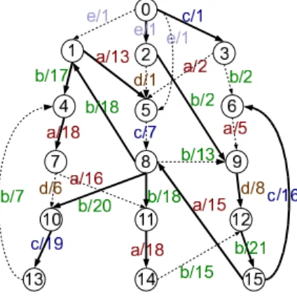
Figure 5 shows each edge in our running example associating with the weight defined in Formula 4. For instance, edge (1,5) has a weight 13, which suggests that if we include this edge in the spanning tree, then, we can save 13 path-labels from those path-label sets reaching 5, i.e.,P
u∈V|M(u,5)−
MT(u,5)
|= 13.
Figure 5: Weighted Graph
Step 2 (Discovering Maximal Directed Spanning Tree):
Given this, the maximal directed spanning tree ofGis de-fined as a rooted directed spanning treeT = (V, ET) [9, 11], whereET is a subset of E such that the sum of w(u,v) for all (u,v) inET is maximized:
T′= arg max
T W(T) = arg maxT
X
(u,v)∈ET
w(u, v),
where W(T) is the total weight of the spanning tree. We can invoke the Chu-Liu/Edmonds algorithm [9, 11] to find the maximal directed spanning tree ofG.
Theorem 3. The maximal directed spanning tree of G,
T′, would minimize the new partial transitive closureMT,
f(T), which is also the upper bound ofN T size:
minTf(T) =f(T′)
Proof Sketch:To prove this, we will show an important equivalent relationship between the new partial transitive closure sizeMT,f(T), and the overall weight of the directed spanning tree
W(T) = X
(v′,v)∈ET
w(v′, v).
Let the size of complete generalized transitive closureM be
cost(M) = X
(u,v)∈V×V
|M(u, v)|
Then, we have for any spanning treeT ofG, the following holds:
f(T) =cost(M)−W(T)
Sincecost(M) is a constant for db-graphG, this equation suggests the minimization off(T) is equivalent to the max-imization ofW(T).
We prove this equation as follows: f(T) =
X (u,v)∈V×V |MT(u, v)|= X (u,v)∈V×V |M(u, v)−Me(u, v)| = X (u,v)∈V×V (|M(u, v)| − |(M(u, v′)⊙ {λ(v′, v)})∩M(u, v)|) = cost(M)− X (u,v)∈V×V |(M(u, v′)⊙ {λ(v′, v)})∩M(u, v)| = cost(M)− X (v′,v)∈E X u∈V |(M(u, v′)⊙ {λ(v′, v)})∩M(u, v)| = cost(M)− X (v′,v)∈E w(v′, v) =cost(M)−W(T) 2
Finally, once the optimal spanning treeT is identified, we can compute the partial transitive closureN T as follows.
Step 3 (Partial Transitive Closure N T): Calculating
N T fromM andT according to Lemma 1.
The total computational complexity of our index construc-tion procedure (Step 1-3) isO(|V|222|Σ|) since the first steps
takesO(|V|(2|Σ|)2), the second step takesO(|E|+|V|log|V|), and the last step takes,O(|V|2(2|Σ|)2) time all in worst case.
4.2
Scalable Index Construction
The aforementioned index construction algorithm relies on the pre-computation of the generalized transitive closure
M, which becomes too expensive for the large graphs. Espe-cially, the storage cost ofMcan easily exceed the size of the main memory and result in memory thrashing. To make our index construction scalable to large graphs, we must avoid the full materialization ofM. Note that the goal of the max-imal spanning tree algorithm is to optimize the total weight of the treeP
(u,v)∈Tw(u, v), which corresponds to the lower bound of the total saving for N T. The research question here is how can we discover a spanning tree whose total weight is close to the total weight of the maximal spanning tree with guaranteed probabilistic bound. Specifically, we formulate the approximate maximal spanning tree problem as follows:
Definition 7. (Approximate Maximal Spanning Tree
Problem) Given a db-graphG, letTo be the optimal span-ning tree ofGwhich has the maximal total weightW(To) = P
(v′,v)∈ETow(u, v). The approximate maximal spanning tree problem tries to find another spanning treeT ofG, such that
with probability of at least1−δ, the relative difference be-tween its total weight W(T) and the maximal tree weight
W(To) is no higher thanθ:
P r(W(To)−W(T)
W(To)
≤θ)≥1−δ. (5)
In this problem, bothǫandδare user-defined parameters to specify the goodness of the approximate maximal span-ning tree. As an example, ifǫ = 1% andδ = 0.1%, then with probability 99.9%, the desired treeT should have a to-tal weight no less than 99% of the toto-tal weight of the exact maximal spanning treeTo, i.e.,W(T)≥99%W(To). Note that the total weight of the approximate spanning tree can not exceedW(To).
In the following, we present a novel algorithm which solves this problem through sampling, thus avoiding the full mate-rialization of the generalized transitive closureM for large graphs. In a nutshell, our algorithm works as follows:
Step 1: We first sample a list of vertices in the db-graph
G.
Step 2: We then compute each of their generalized tran-sitive closure inG, i.e., for a sample vertexu, we compute
M(u, v) for each vertex v in the graph. The latter is re-ferred to assingle-source transitive closureproblem and can be solved efficiently.
Step 3: We use the single-sourceM(u, v) from those sample vertices to estimate the exact edge weight (w(v′, v), Formula
(4)) and the error bound (confidence interval) for such es-timation. Specifically, we leverage the combinedHoeffding and Bernstein boundsfor the error bound estimation. Given this, each edge is associated with two values, one for the es-timated weight and another for the error bound.
Step 4:we discover two maximal spanning trees in the db-graphGbased on each of these two values as edge weight assignment.
Step 5:we introduce a simple test condition using the total weights of these two trees to determine if the criterion (5) is satisfied. If the answer is no, we will repeat the above steps until the test condition holds. We refer to this algorithm as Hoeffding-Bernstein-Tree, as it utilizes Hoeffding and Bern-stein Bounds [13, 23] to determine the stop condition of a sampling process. In the reminder of this subsection, we will detail the key steps in this algorithm.
Sampling Estimator with Hoeffding and Bernstein Bounds
.
Recall the edge weightw(v′, v) =X
u∈V
|(M(u, v′)⊙ {λ(v′, v)})∩M(u, v)|
In our algorithm, an important ingredient is to utilize sam-pling and statistical bounds (Hoeffding and Bernstein Bounds) to provide an accurate estimation of each edge weight in the graph. The key observation which enables a sampling based estimator forw(v′, v) is that w(v′, v) is the sum of
|V|individual quantities,|(M(u, v′)⊙ {λ(v′, v)})∩M(u, v)|.
This gives rise to this question: assuming we haven sam-plesu1, u2,· · ·, un, and for each sample vertex ui, can we compute efficiently each individual term
Xe,i=|(M(ui, v′)⊙ {λ(v′, v)})∩M(ui, v)| (6)
Here, we utilize sampling with replacement to simplify the statistical inference. We also focus on approximating this quantity for convenience:
Xe=w(v′, v)/|V|,wheree= (v′, v)∈E(G). (7)
Note that since each edge weight (and error) is divided by the same constant|V|, the bounds for relative difference on the (total) edge weight remains the same. Indeed, we may think of the originalw(v′, v) as the population sum and the new quantityXe is the population mean, where the weight of a quantityuin the population is|(M(u, v′)⊙{λ(v′, v)})∩ M(u, v)|.
Given this, we define the sampling estimator ofXe as
ˆ Xe,n=1 n n X i=1 Xe,i (8)
Note that for each sample Xi, E(Xe,i) = Xe, and Xi is a bounded random variable, i.e., Xi ∈ [0, R] where R = ` |Σ|
⌊|Σ|/2⌋
´ .
As we mentioned earlier, during the sampling process, each edge e is maintained with two values, one is the es-timated edge weight ˆXe,n, and the other is the error bound
ǫe,n. Using the classical Hoeffding inequality [14], the de-viation (error bound) of the empirical mean from the true expectation (Xe) is: with probability of at least 1−δ′,
|Xˆe,n−E( ˆXe,n)|=|Xˆe,n−E(Xe,i)|=|Xˆe,n−Xe| ≤R
s
lnδ2′
2n
However, this bound is rather loose as it decreases according to√n. Recently, the Hoeffding bound has been improved by incorporating theempirical Bernstein bound[13, 23], which depends on only the empirical standard deviation:
ˆ σ2e,n= 1 n n X i=1 (Xe,i−Xˆe,n)2=1 n( n X i=1 Xe,i2 −Xˆe,n2 ) (9)
The combined Hoeffding and Bernstein bound is expressed as:
P r(|Xˆe,n−Xe| ≤ǫe,n)≥1−δ′, ǫe,n= ˆσ2e,n
s 2 ln 3 δ′ n + 3Rln3 δ′ n (10)
Here, the dependency of the rangeRin the error termǫe,n decreases linearly with respect to the sample sizen. The er-ror term also depends on σˆ
2 e,n
√n. However, since the empirical standard deviation ˆσe,n2 is typically much smaller than the rangeR, this bound is tighter than the Hoeffding bound. In our algorithm, we use the Hoeffding and Bernstein bound (10) as our error bound. Note that both the estimated edge weight ˆXe,nand the error boundǫe,ncan be easily incremen-tally maintained (without recordingXe,ifor each sampleui and edge e). We simply record the following two sample statistics, Pni=1Xe,i and Pni=1Xe,i2 . For the error bound determination (10), we need choose δ′, which in our
algo-rithm is specified asδ′= δ
|E|. By setting up this confidence
level, we can easily derive the following observation: Lemma 2. Given n sample vertices and δ′ = δ
|E|, with
probability more than1−δ, the deviation of each estimated edge weight Xˆe,n in the graph from their exact edge weight
Xe is no greater than the error bound defined in (10):
P r( ^
e∈E(G)
|Xˆe,n−Xe| ≤ǫe,n)≥1−δ. (11)
This can be easily proven by the Bonferroni inequality. Lemma 2 also suggests a computation procedure we can use to esti-mate each edge weight. Basically, assuming we haven sam-ples,u1, u2,· · ·, un, for each sample vertexui, we will com-pute thesingle-source generalized transitive closure,M(ui, v), for any vertexv∈V. From there, we can calculateXe,ifor each edgeein the graph.
Approximate Maximal Spanning Tree Construction
.
Assuming we haven sample vertices, the above discussion describes that each edge in the graph is associated with two values, the estimated weight ˆXe,nand its error boundǫe,n. Given this, our algorithm then will discover two maximal spanning trees in the db-graphG, treeT for the estimated edge weight ˆXe,nassignment and treeT′for the error bound
ǫe,nassignment. Under what condition, can we tell that tree
T would be the desired tree which meet the criterion (5)? Theorem 4 provides a positive answer to this question.
Theorem 4. Givennsamples, letT be the maximal span-ning tree of Gwhere each edge e has weight Xˆe,n, and let
T′ be the maximal spanning tree of Gwhere each edge has weightǫe,n. We denoteWn(T) =Pe∈TXˆe,nand∆n(T′) = P
e′∈T′ǫe′,n. Then, if T satisfies (12), then T is our ap-proximate tree: 2∆n(T′) Wn(T)−∆n(T′) ≤θ, whereWn(T)≥∆n(T′), (12) =⇒P r(W(To)−W(T) W(To) ≤θ)≥1−δ.
Proof Sketch:First, we have
P r(|Wn(T)−W(T)| ≤∆n(T′))≥1−δ This is because with probability of at least 1−δ,
|Wn(T)−E(Wn(T))|=| X e∈T ˆ Xe,n− X e∈T E( ˆXe,n)|= |X e∈T ( ˆXe,n−Xe)|=|Wn(T)−W(T)| ≤ X e∈T ǫe,n(Lemma2)
≤∆n(T′)(∆n(T′) is the maximal total error of any tree inG) Similarly, from Lemma 2, this also holds:
P r(|Wn(To)−W(To)| ≤∆n(T′))≥1−δ. In addition, by definition, we have
Wn(To)≤Wn(T) andW(To)≥W(T). Putting them together, we have
P r(Wn(T)−∆n(T′)≤W(T)≤W(To)≤Wn(T)+∆n(T′))≥1−δ. Thus, the following hold:
P r(W(To)−W(T)≤2∆n(T′))≥1−δ(13)
P r(Wn(T)−∆n(T′)≤W(To))≥1−δ(14)
Finally, if 2∆n(T′)
Wn(T)−∆n(T′) ≤θ(12), with(13)and(14) =⇒ with probability of at least 1−δ, W(To)−W(T)
W(To)
≤ 2∆n(T′)
Wn(T)−∆n(T′)
≤θ 2
Overall Algorithm
.
The sketch of the Hoeffding-Bernstein-Treealgorithm is illustrated in Algorithm 2. This algorithm performs in a batch fashion. In each batch, we sample n0 vertices. Lines 3−4 correspond to the sampling step (Step 1); Lines 5−11 describe thesingle-source transitive closure computation for each sampled vertex (Step 2); Lines 12−15 compute the two values for each edge, the estimated edge weight and its error bound (Step 3); Lines 16 and 17 find the maximal spanning trees for edge value (step 4); and fi-nally, Line 18 tests if these two trees satisfy the conditionAlgorithm 2Hoeffding-Bernstein-Tree(G(V, E,Σ, λ) 1: n←0{n0is the initial sample size}
2: repeat
3: S←SampleV ertices(V, n0){samplen0vertices inV} 4: n←n+n0{nis the total number of samples}
5: for eachui∈Sdo
6: Mi←SingleSourceP athLabel(G, u)
7: for eache∈E{e= (v′, v)}do
8: Xe,i← |(Mi[v′]⊙ {λ(v′, v)})∩Mi[v]| {Formula (6)}
9: UpdatePn
i=1Xe,iandPni=1Xe,i2
10: end for
11: end for
12: for eache∈E {e= (v′, v)}do
13: Xˆe,n←n1Pni=1Xe,i{edge weight estimator (8)} 14: ǫe,n←σˆe,n2 r 2 ln 3 δ′ n + 3Rln 3 δ′ n {error bound (10)} 15: end for
16: T ←M ST(G,[ ˆXe,n]){Maximal Spanning Tree with ˆXe,n
as edge weight}
17: T′←M ST(G,[ǫe,n]){ǫe,nas edge weight}
18: untilCondition (12)=true
Procedure SingleSourcePathLabel(G(V, E,Σ, λ),u) 19: M←∅;V1← {u}; 20: whileV16=∅do 21: V2←∅; 22: for eachv∈V1do 23: for eachv′∈N(v){v′∈N(v) : (v, v′)∈E}do 24: N ew←Prune(M[v′]S M[v]⊙ {λ(v, v′)}); 25: ifN ew6=M[v′]then 26: M[v′]←N ew;V2←V2∪ {v′}; 27: end if 28: end for 29: end for 30: V1←V2; 31: end while
described in Formula (12). The batch sampling reduces the invocation of MST (directed maximal spanning tree algo-rithm). The batch sample size n0 is adjustable and does not affect the correctness of this algorithm. For very large graphG, we typically setn0 = 100. As later we will show in the experimental results, the choice ofn0does not signif-icantly affect the running time due to the relatively cheap computational cost of the maximal spanning tree algorithm. TheSingleSourcePathLabelprocedure is for computing the generalize transitive closure from a single vertex u. This procedure is essentially a generalization of the well-known Bellman-Ford algorithm for the shortest path computation [10]. The procedure works in an iterative fashion. In set V1, we record all the vertices whose path-label sets have been changed (Lines 25−26, and 30) in the current iteration. Then in the next iteration, we visit all the direct neighbors of vertices in V1 and modify their path-label sets accord-ingly (Lines 22−29). For the single source computation,V1 is initialized to contain only the single vertexu. The proce-dure will continue until no change occurs for any path-label sets (V1 =∅). It is easy to see that the maximal number of iteration is |V|by considering the longest path vertex u
can reach is|V|steps. Thus, the worst case computational complexity ofSingleSourcePathLabelis O(|V||E|` |Σ|
|Σ|/2 ´
). Given this, we can see that the total computational com-plexity for Hoeffding-Bernstein-Tree is O(n|V||E|` |Σ|
|Σ|/2 ´
+
n/n0(|E|+|V|log|V|)). The first term comes from the sin-gle source generalized transitive closure computation and the second term comes from the maximal spanning tree
al-gorithms. Clearly, the first term is the dominant part. How-ever, since the sample size is typically quite small (as we will show in the experimental evaluation), the Hoeffding-Bernstein-Treealgorithm is very fast. In addition, this al-gorithm has very low memory requirement as we need tem-porarily store the intermediate results of the SingleSour-cePathLabelfor only a single vertex. We note that this algo-rithm would work well when the total label size|Σ|is small. Since the sampling error bound is in the linear order of`|Σ|
2 ´
, when the number of distinct labels is large, the sampling size can easily exceed the total number of vertices in the graph. In this case, instead of sampling, we can simply compute the single source path label set for each vertex in the graph, and then maintainPni=1Xe,i. Therefore, in both cases, we can completely eliminate the memory bottleneck due to the fully materialization of the generalized transitive closureM
for generating the spanning tree.
Finally, we note that after the spanning treeT is derived, we need to compute the partial transitive closure N T. In Step 3 of the original index construction (Subsection 4.1), we rely on Lemma 1 and still need the generalized transitive closure M. In the following, we describe a simple proce-dure which can compute thesingle source partial transitive closure, i.e,N T(u, v) of vertexufor eachv∈V. The idea is similar to the aforementionedSingleSourcePathLabel algo-rithm. However, instead of maintaining only one path-label set for each vertexvfromu, denoted asM[v] (corresponding
M(u, v)) in SingleSourcePathLabel, we will maintain three path-label sets based on Definition 4: 1)Ms[v] corresponds to Ms(u, v) which records all the path-labels from u to v
with first edge being a tree-edge; 2)Me[v], corresponds to
Me(u, v)−Ms(u, v), which records all the path-labels from
uto v with last edge being a tree-edge and first edge be-ing a non-tree edge; and 3)N T[v], corresponds toN T(u, v), which records the path-labels from u to v with both first edge and last edge being non-tree edges. Note that since each set is uniquely defined by either the first and/or last edge type in a path, we can easily maintain them during the computation ofSingleSourcePathLabel algorithm. Basi-cally, we can compute theN T for each vertex in turn, and it has the same computational complexity as the SingleSour-cePathLabelalgorithm. Due to the space limitation, we omit the details here.
5.
FAST QUERY PROCESSING
In this section, we study how to use the spanning treeT
and partial transitive closure N T to efficiently answer the LCR queries. Using Theorem 2, we may easily derive the following procedure to answer a LCR query (u−→A v): 1) we perform a DFS traversal of the sub-tree rooted atuto findu′ ∈Succ(u), where L(P
T(u, u′))⊆ A; 2) for a given
u′, we check each of its neighborsv′in the partial transitive
closure, i.e., N T(u′, v′) =6 ∅ and v′ ∈ P red(v), to see if
N T(u′, v′) contains a path-label which is a subset ofA; and
3) for thosev′, we check ifL(P
T(v′, v))⊆A. In other words, we try to identify a path-label which is a subset ofAand is represented by three parts, the beginning in-tree path-label
L(PT(u, u′)), the non-tree partN T(u′, v′), and the ending in-tree partL(PT(v′, v)).
This procedure, however, is inefficient since the partial transitive closure is very sparse, and many successors ofu
do not link to any of v’s predecessor through N T.
More-over, the size of u’s successor set can be very large. This leads to the following question: can we quickly identify all the (u′, v′), whereu′∈Succ(u) andv′∈P red(v), such that N T(u′, v′)6=∅? The second important question we need to address is how to efficiently compute the in-tree path-labels,
L(PT(u, u′)) and L(PT(v′, v)). This is a key operation for the query processing for a LCR query, and we apparently do not want to traverse the in-tree path from the starting vertex, such asu, to the end vertex, such asu′, to construct
the path-label. If we can answer these two questions posi-tively, how can we utilize them to devise an efficient query answering procedure for LCR queries? We investigate these questions in the following subsections.
5.1
Searching Non-Empty Entry of NT
In this subsection, we will derive an efficient algorithm by utilizing a multi-dimensional geometric search structure to quickly identify non-empty entries of the partial transitive closure: i.e., given two verticesuandv, quickly identify all the vertex pairs (u′, v′), u′ ∈ Succ(u) and v′ ∈ P red(v),such that N T(u′, v′)6=∅.
The straightforward way to solve this problem is to first find allu’s successors (Succ(u)) andv’s predecessors (P red(v)), and then test each pair of the Cartesian productSucc(u)×
P red(v), to see whether the corresponding entry in N T is
not empty. This method hasO(|Succ(u)| × |P red(v)|) com-plexity, which is clearly too high.
Our new approach utilizes the interval-labeling scheme [12] for the spanning tree T. We perform a preorder traver-sal of the tree to determine a sequence number for each vertex. Each vertex u in the tree is assigned an interval:
[pre(u), index(u)], wherepre(u) isu’spreordernumber and
index(u) is the highest preorder number of u’s successors.
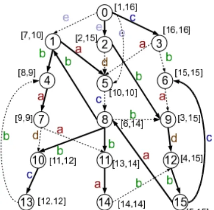
Figure 6 shows the interval labeling for the spanning tree in Figure 3. It is easy to see that vertexuis a predecessor of vertexviff[pre(v), index(v)]⊆[pre(u), index(u)] [12].
The key idea of our new approach is to utilize the span-ning tree to transform this search problem into a geometric range-search problem. Simply speaking, we map each non-empty entry (u′, v′) of NT into a four-dimensional point and
convert the query verticesuandvinto an axis-parallel range. We describe our transformation and its correctness using the following theorem.
Theorem 5. Let each pair (u′, v′), whereN T(u′, v′)6=∅, be mapped to a four-dimensional point (pre(u′),index(u′),
pre(v′),index(u′)). Then, for any two query verticesuand
v, the vertex pair (u′, v′), u′ ∈ Succ(u) and v′ ∈ P red(v),
such thatN T(u′, v′)6=∅, corresponds to a four-dimensional
point (pre(u′), index(u′), pre(v′), index(v′)) in the range: [pre(u), index(u)],[pre(u),index(u)],[1, pre(v)],[index(v),|V|] of a four-dimensional space.
Proof Sketch:We will show that for anyN T(u′, v′) 6=∅,
(pre(u′),index(u′),pre(v′),index(v′)) is in the range,pre(u′)∈ [pre(u),
index(u)],index(u′)∈[pre(u),index(u)],pre(v′)∈[1, pre(v)], index(v′)∈[index(v),|V|] iffu′∈Succ(u) andv′∈P red(v).
Figure 6: Interval Labeling for Spanning Tree
Figure 7: Coordinates in 4-dimensions
pre(u)≤pre(u′)≤index(u) and
pre(u)≤index(u′)≤index(u)⇐⇒
ˆ
pre(u′), index(u′)˜
⊆[pre(u), index(u)]⇐⇒u′∈Succ(u)
1≤pre(v′)≤pre(v) and
index(v)≤index(v′)≤ |V| ⇐⇒
ˆ
pre(v′), index(v′)˜
⊇[pre(v), index(v)]⇐⇒v′∈P red(v)
2
Figure 7 give the 4-dimension coordinates (pre(u′), index(u′),
pre(v′), index(v′)) for each NT (u′, v′). For example,
con-sider a query (u, v) on graphGwith spanning tree given as in Figure 6, whereu= 11 andv= 6. There is a vertex pair (u′, v′) where N T(u′, v′) = {c} and u′ = 14 and v′ = 12 such thatu′ ∈Succ(u) andv′ ∈Succ(v). It is easy to
ver-ify (pre(u′), index(u′),pre(v′), index(v′)), which is (14,14,
4,15) within the range [pre(u),
index(u)], [pre(u),index(u)], [1, pre(v)], [index(v),|V|]. This transformation allows us to apply the test conditions for both the successors ofuand the predecessors ofv simul-taneously, and those test conditions correspond to a multi-dimensional range search. Using a kd-tree or range search tree, we can efficiently index and search all the points in an
axis-parallel range [5]. Specifically, the construction of kd-tree takes O(nlog2n), and querying an axis-parallel range in a balanced kd-tree takesO(n3/4+k) time (in four dimen-sional space), wherenis the total number of pairs with non-empty entries in NT, and k is the number of the reported points. The range-search tree provides faster search time. It can be constructed in O(nlog3d) time and answers the query withO(log4n+k) time (for four dimensional space).
5.2
Computing In-Tree Path-Labels
In this subsection, we present ahistogram-based technique to quickly compute the path-label of an in-tree path. Letx
and y be two vertices in a tree T where x is y’s ancestor,
x∈P red(y). Our goal is to compute the path-label set of
the in-tree path from xto y, L(PT(x, y)), very fast. We build a histogram for each vertex in tree T. Let r be the root vertex ofT. Then, the histogram of vertexu, denoted as H(u), records not only each unique label in the in-tree path from the root vertex to u, i.e., L(PT(r, u)), but also the number of edges in the path containing each label. For instance, the histogram for vertex 14 in Figure 3 isH(14) = {b: 1, d: 2, e: 2}and the histogram for vertex 6 is H(6) = {a: 2, b: 2, c: 1, d: 1, e: 1}. Clearly, a simple DFS traversal procedure can construct the histogram for each vertex ofT
inO(|V||Σ|).
We can compute the path-label sets from vertexutovby subtracting the corresponding counters inH(u) fromH(v). Specifically, for each edge label inH(v), we will subtract its counter inH(v) by the counter of the same label in H(u), if it exists. If the counter of the same label does not appear in H(u), we treat the counter as 0. Given this, the path-label set from uto vinclude all the labels whose resulting counter is more than 0, i.e., we know that there is an edge with this label on the in-tree path fromutov. Clearly, this approach utilizesO(|V||Σ|) storage and can compute an in-tree path-label in O(|Σ|) time, where|Σ|is the number of distinct labels in treeT. Since the number of possible labels, |Σ|, is typically small, and can be treated as a constant, this approach can compute the path-label for any in-tree path very fast.
5.3
LCR Query Processing
Here, we present a new algorithm for fast LCR query processing which utilizes the new technique for efficiently searching non-empty entries in N T developed in last sub-section. The sketch of the algorithm is in Algorithm 3. For a LCR query (u →A v), in the first step (Line 1), we search for all the vertex pairs (u′, v′), where u′ ∈ Succ(u)
andv′∈P red(v), such thatN T(u′, v′)6=∅. We can achieve
this very efficiently by transforming this step into a geomet-ric search problem and then utilizing a kd-tree or range-search tree to retrieve all targeted pairs. We put all these pairs in a listL. Then, we test each vertex pair (u′, v′) in L to see if we can construct a path-label using these three segments,PT(u, u′),N T(u′, v′) andP
T(v′, v). Here, the in-tree path-label is computed using the histogram-based ap-proach. Thus, we first test if the in-tree path-label sets,
L(PT(u, u′)) and L(PT(v′, v)) are subsets of A, and then check ifN T(u′, v′) contains a path-label set which is a
sub-set ofA.
We aggressively prune those (u′, v′) pairs which will not
be able to connect u to v with label constraint A. This is done in Lines 10 and 13. Note that when L(PT(u, u′))