How Caching Affects Hashing
∗Gregory L. Heileman
[email protected]
Department of Electrical and Computer Engineering
University of New Mexico, Albuquerque, NM
Wenbin Luo
[email protected]
Engineering Department
St. Mary’s University, San Antonio, TX
Abstract
A number of recent papers have considered the influence of modern computer memory hierarchies on the performance of hashing algorithms [1, 2, 3]. Motivation for these papers is drawn from recent technology trends that have produced an ever-widening gap between the speed of CPUs and the latency of dynamic random access memories. The result is an emerging computing folklore which contends that inferior hash functions, in terms of the number of collisions they pro-duce, may in fact lead to superior performance because these collisions mainly occur in cache rather than main memory. This line of reasoning is the antithesis of that used to jus-tify most of the improvements that have been proposed for open address hashing over the past forty years. Such im-provements have generally sought to minimize collisions by spreading data elements more randomly through the hash table. Indeed the name “hashing itself is meant to con-vey this notion [12]. However, the very act of spreading the data elements throughout the table negatively impacts their degree of spatial locality in computer memory, thereby increasing the likelihood of cache misses during long probe sequences. In this paper we study the performance trade-offs that exist when implementing open address hash func-tions on contemporary computers. Experimental analyses are reported that make use of a variety of different hash functions, ranging from linear probing to highly “chaotic forms of double hashing, using data sets that are justified through information-theoretic analyses. Our results, con-trary to those in a number of recently published papers, show that the savings gained by reducing collisions (and therefore probe sequence lengths) usually compensate for any increase in cache misses. That is, linear probing is usually no better than, and in some cases performs far worse than double hash functions that spread data more randomly through the table. ∗We wish to thank to Bernard Moret for suggesting this topic
to us.
Thus, for general-purpose use, a practitioner is well-advised to choose double hashing over linear probing. Explanations are provided as to why these results differ from those previ-ously reported.
1 Introduction.
In the analysis of data structures and algorithms, an abstract view is generally taken of computer memory, treating it as a linear array with uniform access times. Given this assumption, one can easily judge two com-peting algorithms for solving a particular problem—the superior algorithm is the one that executes fewer in-structions. In real computer architectures, however, the assumption that every memory access has the same cost is not valid. We will consider the general situation of a memory hierarchy that consists of cache memory, main memory, and secondary storage that is utilized as vir-tual memory. As one moves further from the CPU in this hierarchy, the memory devices become slower as their capacity become larger. Currently, the typical sit-uation involves cache memory that is roughly 100 times faster than main memory, and main memory that is roughly 10,000 times faster than secondary storage [10]. In our model of the memory hierarchy, we will treat cache memory as a unified whole, making no distinc-tion between L1 and L2 cache.
It is well known that the manner in which memory devices are utilized during the execution of a program can dramatically impact the performance of the pro-gram. That is, it is not just the raw quantity of memory accesses that determines the running time of an algo-rithm, but the nature of these memory accesses is also important. Indeed, it is possible for an algorithm with a lower instruction count that does not effectively use cache memory to actually run slower than an algorithm with a higher instruction count that does make efficient
use of cache. A number of recent papers have considered this issue [1, 2, 13, 14], and the topic of “cache-aware” programming is gaining in prominence [4, 6, 15].
In this paper we conduct analyses of open address hashing algorithms, taking into account the memory ac-cess patterns that result from implementing these algo-rithms on modern computing architectures. We begin in Section 2 with a description of open address hashing in general, and then we present three specific open address hashing algorithms, including linear probing, linear dou-ble hashing, and exponential doudou-ble hashing. We dis-cuss the memory access patterns that each of these algo-rithms should produce when implemented, with particu-lar considerations given to interactions with cache mem-ory. These access patterns have a high degree of spatial locality in the case of linear probing, and a much lower degree of spatial locality in the case of double hashing. Indeed, the exponential double hashing algorithm that we describe creates memory access patterns very simi-lar to those of uniform hashing, which tends to produce the optimal situation in terms of memory accesses, but is also the worst case in terms of spatial locality.
In Section 3 previous research results dealing with open addressing hashing are presented. First we de-scribe theoretical results that show double hashing closely approximates uniform hashing, under the as-sumption that data elements are uniformly distributed. It was subsequently shown experimentally that the per-formance of linear double hashing diverges significantly from that of uniform hashing when skewed data dis-tributions are used, and that in the case of exponen-tial double hashing this divergence is not as severe [20]. Thus, exponential double hashing is the best choice if the goal is to minimize the raw number of memory ac-cesses. These results, however, do not consider how cache memory may impact performance. Thus in Sec-tion 3 we also review a number of recent experimental results that have been used to make the case that, due to modern computer architectures, linear probing is gen-erally a better choice than double hashing. We provide detailed analyses of these studies, pointing out the flaws that lead to this erroneous conclusion.
It is important to note that dynamic dictionary data sets are often too small to be directly used to test cache effects. For example, the number of unique words in the largest data set available in the DIMACS Dictionary Tests challenge,joyce.dat, will fit in the cache memory of most modern computers. Thus, in Section 4 we de-scribe an information-theoretic technique that allows us to create large synthetic data sets that are based on real data sets such asjoyce.dat. These data sets are there-fore realistic, yet large enough to create the cache effects necessary to study the performance of linear probing
and double hashing on modern architectures. This is followed in Section 5 by a description of a set of exper-iments that used these synthetic data sets to measure the actual performance of the aforementioned hashing algorithms. Three important performance factors con-sidered are the number of probes (and therefore memory accesses) required during the search process, the num-ber of cache misses generated by the particular probe sequence, and the load factor of the hash table. In ad-dition, we also consider how the size of the hash table, and the size of the data elements stored in the hash ta-ble affect performance. In general, hash functions that produce highly random probe sequences lead to shorter searches, as measured by the number of memory ac-cesses, but are also more likely to produce cache misses while processing these memory access requests. Our ex-periments were aimed at quantifying the net affects of these competing phenomena, along with the impact of the other performance factors we have just mentioned, on the overall performance of open address hashing algo-rithms. The results, presented in Section 5, show that it is difficult to find cases, either real or contrived, whereby linear probing outperforms double hashing. However, it is easy to find situations where linear probing performs far worse than double hashing, particularly when real-istic data distributions are considered.
2 Open Address Hashing.
We assume hashing with open addressing used to resolve collisions. The data elements stored in the hash table are assumed to be from the dynamic dictionaryD. Each data element x∈Dhas a key valuekx, taken from the
universeU of possible key values, that is used to identify the data element. The dynamic dictionary operations of interest include:
• Find(k, D). Returns the elementx∈D such that
kx=k, if such an element exists.
• Insert(x, D). Adds element xto Dusing kx.
• Delete(k, D). Removes the element x ∈ D that satisfieskx=k, if such an element exists.
When implementing these operations using a hash table with m slots, a table index is computed from the key value using aordinary hash function, h, that performs the mapping h: U → ZZm, where ZZm denotes the set
{0,1, . . . , m−1}.
Hashing with open addressing uses the mappingH:
U×ZZ→ZZm, where ZZ ={0,1,2, . . .}, and produces the
probe sequence < H(0, k), H(1, k), H(2, k), . . . > [18]. For a hash table containing m slots, there can be at most m unique elements in a probe sequence. A full length probe sequence visits allmhash table locations using onlymprobes. One of the key factors affecting the
length of a probe sequence needed to implement any of the dynamic dictionary operations is the load factor,
α, of the hash table, which is defined as the ratio of the number of data elements stored in the table to the number of slots,m, in the hash table.
Next, we describe three specific probing strategies. For each of these, we first describe the generic family of hash functions associated with the strategy, and then we consider the particular implementations used in our experiments.
2.1 Linear Probing. The family of linear hash func-tions (linear probing) can be expressed as
HL(k, i) = (h(k) +ci) modm,
(2.1)
where h(k) is an ordinary hash function that maps a key to an initial location in the table,i= 0,1, . . .is the probe number, and c is a constant. This technique is known as linear probing because the argument of the modulus operator is linearly dependent on the probe number. In general, c needs to be chosen so that it is relatively prime to m in order to guarantee full-length probe sequences. For the most common case, whenc= 1, this hash function will simply probe the sequential locations < h(k) modm,(h(k) + 1) modm, . . . , m −
1,0,1, . . . ,(h(k)−2) modm,(h(k)−1) modm >in the hash table. Whenever we use HL in this paper we are
assumingc= 1.
The ordinary hash function h(·) used in equa-tion (2.1) has a dramatic impact on the performance of linear probing. A common choice is
h(k) =kmodm.
(2.2)
Furthermore, if the keys are uniformly distributed, then statistically this ordinary hash function is optimal in the sense that it will minimize collisions. This is be-cause for each key the initial probe into the hash table will follow the uniform distribution. When using equa-tion (2.2) with linear probing, performance degrades rapidly as the key distribution diverges from the uni-form distribution. Two approaches are commonly used to address this problem. First, one can apply a random-izing transformation to the keys prior to supplying them to equation (2.2). This is actually a natural step to take in many applications. For example, consider compiler symbol tables, where strings must be converted into nu-meric key values in order to “hash” them into the table. One such popular algorithm, calledhashPJW(), takes a string as input, and output an integer in the range [0,232−1] [1]. The transformation performed by hash-PJW() tends to do a good job of producing numbers that appear uniform over [0, m], even when the strings being hashed are very similar.
A second approach involves using a more compli-cated ordinary hash function h(·) so that the initial probe into the hash table is more random. In addi-tion, by randomizing the choice of h(·) itself we can guarantee good average-case performance (relative to any fixed ordinary hash function) through the use of
universal hashing [5]. A family of ordinary hash func-tionsηis said to be universal if for each pair of distinct keys kα, kβ ∈ U, the number of hash functions h ∈ η
for whichh(kα) =h(kβ) is at most|η|/m. For example,
the following is a universal hash function
h(k) = ((ak+b) modp) modm
(2.3)
where a ∈ ZZ∗p and b ∈ ZZp are chosen at random,
ZZ∗p denotes the set {1,2, . . . , p−1}, and p is a prime
number large enough so that every possible k∈U is in [0, p−1]. Thus, for fixed pand m, there are p(p−1) different hash functions in this family. We will make use of this family of universal ordinary hash functions in subsequent experiments.
The limitations of linear probing are well known— namely that it tends to produce primary and secondary clustering. Note, however, that this clustering problem is counterbalanced by the fact that when c = 1, the probing that must be performed when implementing any of the dynamic dictionary operations will be to successive locations, modulom, in the hash table. Thus, if the hash table is implemented in the standard way, using a data structure that maps hash table locations to successive locations in computer memory, then the memory accesses associated with these probes should lead to a high percentage of cache hits.
2.2 Linear Double Hashing. Given two ordinary hash functionsh(k) andg(k), the family of linear double hash functions can be written as
HLD(k, i) = (h(k) +ig(k)) modm.
(2.4)
For a particular keyk, the values ofh(k) andg(k) in the previous equation can be thought of as constants. That is, once a key is selected for use in probing the hash table, the probe sequence is determined byHLD(k, i) =
(ch +icg) modm, where ch = h(k) and cg = g(k).
This is the same form as linear probing described in equation (2.1). Thus, if cg is relatively prime tom, all
probe sequences are guaranteed to be full length. That is,g(k) should be chosen in such a way that the values it produces are always relatively prime to m. The easiest way to assure this is to choose m as a prime number so that any value of g(k) in the range [0, m−1] will be relatively prime tom.
The key advantage of linear double hashing over linear probing is that it is possible for both h(k) and
g(k) to vary withk. Thus, inHLD the probe sequence
depends on k through both h(k) and g(k), and is linear in h(k) and g(k). A widely used member of
HLD proposed by Knuth [12] is h(k) = kmodm and g(k) = kmod (m−2), with m prime. In this paper we will assume the use of these ordinary hash functions withmprime whenever we mentionHLD.
2.3 Exponential Double Hashing. The exponen-tial double hashing family was iniexponen-tially proposed by Smith, Heileman, and Abdallah [20], and subsequently improved by Luo and Heileman [17]. The improved ver-sion that we will consider is given by
HE(k, i) = h(k) +aig(k)modm,
(2.5)
where a is a constant. It has been shown that if m
is prime, and a is a primitive root of m, then all probe sequences produced by this hash function are guaranteed to be full length [17]. A member ofHE that
performs well is obtained by choosing the ordinary hash functionsh(k) =kmodmandg(k) =kmod (m−2) in equation (2.5), withmonce again prime. In this paper we will assume the use of these ordinary hash functions withmprime whenever we mentionHE.
Let us consider the types of memory access pat-terns that should result from the proper implementa-tion of hash funcimplementa-tions from the families HL, HLD and HE. Specifically, members of HL will probe
succes-sive locations in a hash table, and therefore on average should produce more cache hits per probe than mem-bers from the other two hash function families. Fur-thermore, members of HE tend to produce more ran-dom probe sequences than members of HLD. Thus, of the three families of hash functions considered, members of HE should produce the fewest number of cache hits
per probe. The randomness of the probe sequences pro-duced by these hash function families is more rigorously considered in [17].
3 Previous Research.
Before discussing our experimental design and results, it is important to consider some of the previous results on this topic that have appeared in the open literature. We start in Section 3.1 by describing results dealing with the randomness of double hashing. These results focus solely on the average probe length of double hashing algorithms, ignoring cache effects. Given the complexities associated with the analysis of programs executing on real computers, particularly when the memory hierarchy is considered, it is difficult to arrive at meaningful theoretical results that include cache effects. Thus, in Section 3.2 we describe some experimental results that measure how the use of cache memory
affects the performance of open address hash functions. We previously described the important trade-off that should be used to evaluate results in this area. That is, whether the savings gained through the reduction in average probe sequence length due to the use of a more “random” hash function is lost due to the corresponding increase in the number of cache misses per probe. Both of the experimental studies described in Section 3.2 seem to validate this claim, thereby leading to the previously mentioned computing folklore regarding linear probing; however, we also describe in Section 3.2 the flaws in these experiments that have led to erroneous conclusions.
3.1 Randomness of Double Hashing. We have al-ready mentioned that if the goal is to minimize the total number of memory accesses, ignoring cache effects, then from a probabilistic perspective, the ideal case for open address hashing isuniform hashing[21, 22]. A uniform hash function always produces probe sequences of length
m (in the table space), with each of the m! possible probe sequences being equally likely. The obvious way of implementing a uniform hash function involves the generation of independent random permutations over the table space for each keyk∈U; however, the compu-tational costs associated with this strategy make it com-pletely impractical. Thus, practical approximations to uniform hashing have been sought. With this in mind, Knuth [12] noted that any good hash function should: (1) be easy to compute, involving only a few simple op-erations, and (2) spread the elements in random fashion throughout the table space. Only those hash functions satisfying these two conditions will be practical for use in implementing dynamic dictionaries. It is not difficult to see that these two conditions are conflicting—it is in general difficult to satisfy one while simultaneously maintaining the other. Knuth [12] has noted that the double hashing strategy, and in particular the one de-scribed by equation (2.4), strikes a reasonable balance between these competing conditions. Furthermore, it has been shown through probabilistic analyses that this hash function offers a reasonable approximation to uni-form hashing [9, 16]. Let us consider these results in more detail.
It can be shown (see [12]) that the average probe length for uniform hashing is 1−1α+O m1
. Guibas and Szemeredi [9] showed that the average probe length for double hashing is asymptotically equivalent to that of uniform hashing for load factors up to approximately 0.319. Later, Lueker and Molodowitch [16] extended this result to load factors arbitrarily close to 1. Both of these results are only valid under a strong uniformity
assumption. Specifically, they assume that for any key
k∈U
P r{(h(k), g(k)) = (i, j)}= 1
m(m−1) (3.6)
for all (i, j), with 0 ≤ i, j ≤ m− 1. Thus, these results only hold under the assumption that the keys will produce hash value pairs that are jointly uniformly distributed over the table space. This is a strong assumption indeed, that is influenced by both the initial data distribution, as well as the choices ofh(k) andg(k). Most data sets are far from uniform, and the widely used choices for h(k) and g(k) e.g., those discussed previously, would have to be considered poor choices if our goal is to satisfy equation (3.6).
The exponential double hashing algorithm de-scribed in Section 2.3, that has been shown through experimental analysis to be superior to the previously proposed methods in the linear double family of hash functions [17, 20]. Specifically, this experimental anal-ysis demonstrated that linear and exponential double hashing algorithms perform similarly (as measured by the average number of collisions) when the data ele-ments are uniformly distributed, but that exponential double hashing is superior to linear double hashing when the data elements are not uniformly distributed.
3.2 Hashing with Cache Effects. First let us con-sider the experiments described in Binstock [1], which contains a good description of the practical uses of hash-ing, along with some references to useful ordinary hash functions that can be used to convert character strings into integers. Two experiments were performed, both involved allocating a large block of memory, and ex-ecuting as many memory reads as there are bytes in the block. In the first experiment these bytes are read randomly, and in the second experiment the bytes are read sequentially. Predictably, the second experiment runs significantly faster than the first. The first ex-periment, however, does not consider the reduction in average probe length that should accompany the ran-dom memory reads, and thus no conclusions should be drawn with regards to the superiority of any one hashing method based on these experiments.
Black, Martel, and Qi have studied the effects of cache memory on basic graph and hashing algo-rithms [2]. In their study of hashing, they considered three basic collision resolution strategies, two of them based on open addressing. One of the open addressing strategies considered was linear probing, as we have de-scribed it in Section 2.1 with c = 1. The other was a double hashing algorithm, the details of which are not provided in their paper. However the authors do refer
to a website containing a link to the full version of the paper [19], and this paper provides the details of their double hashing algorithm. Specifically, the authors in-troduced the hash function
HBMQ(k, i) = (h(k) +i(c−g(k)) modm,
(3.7)
with h(k) = kmodm and g(k) = kmodc, where
c is a prime less than m. Note that for c = 1, this hash function reduces to linear probing. The authors mention that they experimented with different values for c, finding that small values led to better performance (we will show later that this choice in fact leads to poor performance). In all of the experiments described in the paper, it appears that m was always selected as some power of 2. Given this double hash function, the authors’ experimental results indicated that linear probing tends to outperform double hashing, particularly when the load factor is less than 80% and the entire hash table does not fit in L1 cache. These results are quite different from the results we obtained using the double hashing functions described in Section 2.2. The difference is explained by the choice of the double hash function used in [2]. Specifically, based on the discussion provided in Section 2 of this paper, it is clear that a simple way to guarantee full length probe sequences in the hash function of equation (3.7) is to makec−g(k) andmrelatively prime to one another. The unfortunate choice ofmas a power of 2, however, means that the condition will be violated wheneverc−g(k) is even. Through experimentation, we have also found that the choice ofc is critical, and that the performance of hash function (3.7) is worst when
c m, and best when c ≈ m. In [2] it was the case that cm. For instance, one set of experiments used
c = 43 and m = 222. Choosing m prime and c ≈ m
should lead to a reduction in the number of collisions produced byHBMQ. Indeed, with these choices it seems
that the performance of HBMQ should be very similar
to that ofHLD.
In order to demonstrate the severity of the problem of choosing c small in equation (3.7), we conducted experiments that measured the number of probes per insertion generated byHL,HLD,HE, andHBMQwhen insertingα·muniformly distributed (i.e., initial probes are uniform) data elements into an initially empty table containing m slots. Note that this would be the same number of probes required to successfully search for all of these data elements after they have been inserted into the hash table. The results form= 400,009 are shown in Table 1. Each entry was obtained by averaging over three separate experiments. The column underH?
BMQ
corresponds to a choice of c= 43, while forHBMQ† the choice was c= 400,007. Note that the average number
α HL HLD HE HBMQ? HBMQ† 0.1 1.06 1.06 1.06 1.06 1.11 0.2 1.12 1.12 1.12 1.16 1.23 0.3 1.21 1.20 1.20 1.32 1.36 0.4 1.33 1.31 1.30 14.89 1.52 0.5 1.50 1.44 1.43 40.78 1.70 0.6 1.75 1.61 1.59 63.67 1.92 0.7 2.16 1.86 1.81 87.23 2.21 0.8 2.98 2.23 2.13 117.31 2.62 0.9 5.38 2.92 2.73 153.13 3.35
Table 1: A comparison of the average number of probes per insertion generated by the hash functionsHL(using
equation (2.2)), HLD, HE, and HBMQ on uniformly
distributed data as the load factor,α, ranges from 10% to 90%. The number of slots in the table for each of these was m = 400,009. For HBMQ? , c = 43, and for
HBMQ† , c= 400,007.
of probes generated byH?
BMQgrows rapidly, relative to HL, HLD, and HE when the load factor exceeds 30%;
however, forHBMQ† the number of probes is similar to that ofHLD, and outperforms linear probing when the
load factor grows above 70%. Furthermore, the choice ofmthat we used in these experiments should actually improve somewhat on the results obtained in [2], as it at least guarantees full length probe sequences. Thus, even if cache effects are not taken into account, linear probing outperforms HBMQ? , and by taking them into account, linear probing’s advantage overHBMQ? increases. For all of the suitably defined double hash functions, however, it can be seen from the table that there is a load factor above which linear probing is inferior in terms of the number of probes it produces. That is, at load factors above 30%, HLD and HE execute fewer probes per
insertion than HL. For these double hash functions it
makes sense to consider whether or not this advantage is lost once cache effects are accounted for. In Section 5 we describe experiments that measure this effect, but first we must consider how more realistic input distributions affect the average probe lengths of these hash functions.
4 Data Distributions.
We have already demonstrated in Table 1 that for the uniform distribution, as the load factor increases, the average probe length per insertion for linear probing grows more rapidly than it does for double hashing. This is a well-known fact, and the reasons for this performance have already been discussed in Section 2. However, note that the divergence in the growth rates of the probe lengths is not too severe—for a 90% load factor, the average probe length for linear probing
is approximately twice that of exponential hashing. An important question is how much worse this effect becomes when more realistic input distributions are used. A complication arises when attempting to find realistic data sets the can be used to measure this effect, along with cache effects. Specifically, if cache effects are to be measured, then the dynamic dictionary must be large enough so that it will not fit entirely in cache memory. Note that in our memory hierarchy model, there is never an advantage to linear probing if the entire dynamic dictionary fits in cache memory. All of the data set that we are aware of that have been used to test dynamic dictionary applications are too small; they easily fit in the cache memories of modern computers. Thus, for our experiments we constructed numerous synthetic data sets that are large enough to produce the desired cache effects. In this paper we report only three: one that is optimal and minimizes cache misses for linear probing (the uniform distribution previously considered), and two nonuniform distributions that are meant to capture that notion of real data sets.
The first of the nonuniform distributions is meant to be fairly benign, while the second is meant to demonstrate how poorly linear probing might perform on certain data sets. Specifically, the first nonuniform distribution we refer to as the “clipped Gaussian” distribution N(m2,m
4)(x), where the initial probe into
the table is drawn randomly according to a Gaussian distribution with mean m/2 and standard deviation
m/4. Furthermore, random initial probes outside the range [0, m−1] are discarded. Thus, the tails of the uniform distribution are discarded, and this clipped Gaussian distribution somewhat resembles a uniform distribution in which the probably mass function has a slight “bulge” in the center of the table. The more severe nonuniform distribution is the “clustered” distribution cβ(x), where β ∈(0,1] corresponds to the
fixed percentage of the hash table that all initial probes will occur to in a random fashion. For example, if
β = 0.5, a contiguous region (modulo the table size) that corresponds to 50% of the hash table is chosen at random, and all initial probes will occur uniformly at random in this region.
Given the questions that invariably arise regarding data synthetic distributions, and their correspondence to real data sets, we have sought ways to justify the choice of the aforementioned data distributions for experimental purposes. Below we make use of information theory in order to demonstrate, from a probabilistic perspective, that these nonuniform data distributions are in fact reasonable data sets. We start by presenting some information-theoretic measures that show how far a particular distribution is from the
uniform distribution. Next we apply these measures to specific real data sets that have been used in other studies, and then we demonstrate that the synthetic data sets we constructed are no worse than these real data sets.
4.1 Information-theoretic Approach. Let X be a random variable with alphabetX ={0,1, . . . , m−1}
and probability mass function p(x) = Pr{X =x}, x∈ X. Consider a uniform distribution of data elements
u(x) over a table of size m; that is, X has a uniform distribution. Then the entropy of X is given by
Hu(X) = −
X
x∈X
p(x) logp(x)
= logm,
where all logarithms are assumed to be base 2, and therefore the units of entropy will be in bits. A information-theoretic quantity commonly used to mea-sure the distance between two probability mass func-tionsp(x) andq(x) is given by the relative entropy (or Kullback Leibler distance) [7], defined as
D(pkq) =X
x∈X
p(x) logp(x)
q(x).
We will use relative entropy as a means of comparing various data distributions with the ideal case of the uniform distribution.
Consider the clustered distribution cβ(x). The
entropy, Hcβ(X), of this distribution is given by
Hcβ(X) = − X x∈X p(x) logp(x) = − β|X | X 1 β−1 |X | log β−1 |X | = logβ|X |.
The relative entropy between cβ(x) and the uniform
distributionuis given by D(cβku) = X x∈X 1 βm log 1 βm 1 m = βm 1 βm log 1 β = −logβ.
Thus, the relative entropy between c0.5(x) and u is 1
bit, while the relative entropy betweenc0.3(x) and uis
1.74 bits.
The entropy of the clipped Gaussian distribution is difficult to determine analytically. Thus, we created an
experimental entropy measure as follows. For a table of size m, 4m initial probes were generated according to the clipped Gaussian distribution. The number of initial probes to each location in the table was then divided by the total number of initial probes in order to generate an experimental probability for each hash table location, and these experimental probabilities were then used to calculate what we refer to as the “experimental entropy” of the distribution. Many of the experiments reported in this paper used hash tables with m = 100,003 and m = 400,009; for these values the experimental entropies HN(m
2,
m
4) are 15.65 and 17.65, respectively,
while the maximum entropies (corresponding to the uniform distribution) for these table sizes are 16.61 and 18.61, respectively. Furthermore, for bothm= 100,007 and m = 400,009, the experimental relative entropy
D(N(m2,m4)ku) = 0.96 bits.
4.2 Real Data Sets. In this section we consider a number of “real” data sets that are used to help justify the selection of the aforementioned synthetic data sets that we used in our experiments. For each of the real data sets described in this section, we considered the case when duplicate words are ignored, which will produce more uniform input distributions. In each experiment, a hash table that is 1.5 times larger than the number of words in the data set was created, the functionhashPJW() was then used to create a key for the word, and a storage location was computed using equation (2.2).1 Note that this corresponds to the set
of initial probes that would occur in filling a table up to a load factor of 66%. As we have described previously, the number of words that hashed to each location was then divided by the total number of words in order to create an experimental probability for that location, and these experimental probabilities were used to calculate the experimental entropy of the data set.
The Bible. The Bible was used as a data set in [1]. The version that we tested [11] has 817,401 words in total, and 13,838 unique words. For|X |= 13,838×1.5,
Hu(X) = 14.34 bits, HN(m
2,
m
4)(X) = 13.96 bits, and Hc0.3(X) = 12.55 bits. The experimental entropy of
the Bible with no repeated words is 13.18 bits, and the experimental relative entropy between this data set and the uniform distribution is 1.16 bits.
United States Constitution. In the United States Constitution there are 7,671 words in total, of which 1,436 are unique. For |X | = 1,436×1.5,
Hu(X) = 11.07 bits, HN(m
2,m4)(X) = 10.69 bits, and
1Experimentally we found that applying universal hashing to
the output produced byhashPJW() has a negligible effect. That is,hashPJW() does a very good job of transforming skewed input distributions into distributions that are close to uniform.
Hc0.3(X) = 9.29 bits. The experimental entropy of the
United States Constitution with no repeated words is 9.86 bits, and the experimental relative entropy between this data set and the uniform distribution is 1.20 bits.
DIMACS Data Set. The largest file in the DI-MACS data set for dictionaries isjoyce.dat[8]. In this data set, 186,452 dynamic dictionary operations are ap-plied to 8,580 unique words. For |X | = 8,580×1.5,
Hu(X) = 13.65 bits, HN(m
2,
m
4)(X) = 13.28 bits, and Hc0.3(X) = 11.86 bits. The experimental entropy of the
unique words in the data set with no repeated words is 12.49 bits, and the experimental relative entropy be-tween this data set and the uniform distribution is 1.16 bits.
Thus, from an information-theoretic perspective, the synthetic data setsHN(m
2,
m
4)(X) andHc0.3(X) do a
good job of modeling the real data sets in the case when repeated words are not allowed. In particular, for every one of the real data sets, D(N(m2,m4) k u) provides a lower bound for the experimental relative entropy be-tween the real data set and the uniform distribution, whileD(c0.3ku) provides an upper bound for the same
quantity. For the case when repeated words are allowed, note thatD(c0.01ku) is less than the experimental
rel-ative entropy between the Bible data set with repeated words and the uniform distribution, but greater than the relative entropy between the United States Consti-tution data set with repeated words and the uniform distribution. Thus, we will use this distribution to study the case when repeated words are allowed.
5 Experimental Design and Results.
In this section we compare the performance of linear probing and double hashing experimentally. From the previous discussions we know that the average search time depends on the average number of probes and the manner in which cache memory is utilized, and that the average number of probes is dependent on the data distribution and the hash function used. Two sets of experiments were designed to measure how these factors influence the performance of hashing algorithms. The first set of experiments, described in Section 5.1, demonstrates how the data distribution influences the average probe length, while the second set of experiments, described in Section 5.2, measures the time required to actually execute these probes on real machines. Thus, the former experiments do not involve cache effects, while the latter experiments account for them.
5.1 Data Distributions Revisited. Table 1 in Sec-tion 3.2 showed the average number of probes per inser-tion generated by the hash funcinser-tionsHL,HLD,HE, and
direct universal α u N c0.3 u N c0.3 0.1 1.06 1.08 1.25 1.11 1.17 1.27 0.2 1.12 1.20 2.01 1.26 1.29 1.61 0.3 1.21 1.40 272.18 1.45 1.50 2.04 0.4 1.33 1.80 20220.80 1.70 1.77 2.62 0.5 1.50 3.41 40156.14 2.03 2.13 3.36 0.6 1.75 2170.37 60123.89 2.48 2.63 4.36 0.7 2.16 11162.53 80138.41 3.17 3.37 5.75 0.8 2.98 23809.26 100135.75 4.42 4.65 7.91 0.9 5.38 37860.20 120125.09 7.55 8.67 12.56
Table 2: A comparison of the average number of probes per insertion generated byHL using equation (2.2),
di-rect insertion, and equation (2.3), universal hashing, for the initial probe. Three distributions were tested: the uniform distribution u, the clipped Gaussian distribu-tionN(m2,m4) and the clustered distributionc0.3 as the
load factor,α, ranges from 10% to 90%. The number of slots in the table for each is m= 100,003.
HBMQ on uniformly distributed keys. For tractability reasons, a uniform data assumption is often used in al-gorithmic analysis, with the hope that the performance of an algorithm does not diverge significantly from the analytical results if this assumption is violated. For in-stance, a uniformity assumption underlies the theoreti-cal results described in Section 3.1. Furthermore, since it is difficult to derive data distributions that capture the essence of so called “real-world” data sets, uniformly distributed data is also commonly used in experimental studies. For example, all of the experiments in Sec-tion 3.2 used uniformly distributed keys. Again, the hope is that these experiments demonstrate some per-formance aspects of the algorithm under consideration that extend in a reasonable way other distributions, in-cluding real-world data sets. In terms of minimizing probe sequence length, it is important to recognize that a uniform data distribution generally represents the op-timal stochastic input distribution. In the set of exper-iments described next, we investigate the performance losses that accompany nonuniform input distributions. These nonuniform input distributions are intended to be more representative of the types of data distributions encountered in practice.
First let us consider the sensitivity of linear prob-ing to the input distribution. Table 2 shows the av-erage number of probes per insertion generated by HL
when using equation (2.2), direct insertion, and equa-tion (2.3), universal hashing, for the initial probe. The results were obtained by averaging over 10 different ex-periments for the direct insertion method, and 50 dif-ferent experiments for universal hashing. Three
distri-butions were tested. Notice that the best performance is obtained for the uniform distribution when direct in-sertion is used; however, when the distribution diverges from the uniform distribution, the performance of di-rect insertion suffers dramatically. For the case of the clipped Gaussian distribution there is an abrupt change in the average probe length once the load factor exceeds 50%, and for the more severe clustered distribution, a similar abrupt change occurs when the load factor ex-ceeds 20%. Next, consider the right side of the table, where the results for universal hashing are presented. Notice that for the case of the uniform distribution, uni-versal hashing, by modifying the input distribution, ac-tually performs worse than direct insertion; however, as would be expected, it offers significant improvements for the nonuniform distributions. Thus, linear probing has an extreme sensitivity to the input distribution that is supplied to it. In addition, although the theoretical re-sults for universal hashing show that on average it leads to good performance, it also produced the largest vari-ance in all of the hash functions experiments we con-ducted (which is why we averaged the results over a larger number of experiments). For example, for the clustered distribution c0.3, at a load factor of 60% the
mimimum probe length was 2.60, the maximum probe length was 14.0, and the standard deviation was 2.20.
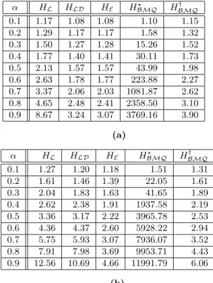
Now let us consider similar experiments that in-clude the double hash functions we have previously dis-cussed (for comparison, we have also included the best results for HL from the previous table). Table 3 lists
the average number of probes per insertion generated by the hash functionsHL,HLD,HE, andHBMQon the
nonuniform hash data distributionsN(m2,m4) and c0.3.
Once again, each entry corresponds to the insertion of
α·mdata elements into an initially empty table contain-ing m slots, and the average is taken over 10 indepen-dent experiments (50 in the case of HL with universal hashing). These experiments are more severe in that they generate a greater number of collisions than the uniform case previously considered.
Hash functionHBMQ was included in these
experi-ments in order to demonstrate it sensitivity to the input distribution if the cparameter is not selected properly. Notice that H?
BMQ has an extreme sensitivity to the
input distribution. As compared to its performance on the uniform distribution (shown in Table 1), its perfor-mance on the clipped Gaussian distribution at a 70% load factor shows a 12-fold increase in probe sequence length, while for the same load factor the increase in probe sequence length for the clustered distribution is 91 times that of its performance on the uniform dis-tribution. Contrast this with HBMQ† , where at a load factor of 70%, for both the clipped Gaussian and the
α HL HLD HE HBMQ? HBMQ† 0.1 1.17 1.08 1.08 1.10 1.15 0.2 1.29 1.17 1.17 1.58 1.32 0.3 1.50 1.27 1.28 15.26 1.52 0.4 1.77 1.40 1.41 30.11 1.73 0.5 2.13 1.57 1.57 43.99 1.98 0.6 2.63 1.78 1.77 223.88 2.27 0.7 3.37 2.06 2.03 1081.87 2.62 0.8 4.65 2.48 2.41 2358.50 3.10 0.9 8.67 3.24 3.07 3769.16 3.90 (a) α HL HLD HE HBMQ? HBMQ† 0.1 1.27 1.20 1.18 1.51 1.31 0.2 1.61 1.46 1.39 22.05 1.61 0.3 2.04 1.83 1.63 41.65 1.89 0.4 2.62 2.38 1.91 1937.58 2.19 0.5 3.36 3.17 2.22 3965.78 2.53 0.6 4.36 4.37 2.60 5928.22 2.94 0.7 5.75 5.93 3.07 7936.07 3.52 0.8 7.91 7.98 3.69 9953.71 4.43 0.9 12.56 10.69 4.66 11991.79 6.06 (b)
Table 3: A comparison of the average number of probes per insertion generated by the hash functionsHL(using
equation (2.3)), HLD, HE, and HBMQ on (a) the
clipped Gaussian distribution N(m2,m4) and (b) the clustered distribution c0.3 as the load factor, α, ranges
from 10% to 90%. The number of slots in the table for each is m= 400,009. ForHBMQ? , c = 43, and for
HBMQ† ,c= 400,007.
clustered distributions, the probe sequence length is not even twice that of the uniform distribution. Thus,
H?
BMQhas an extreme sensitivity to the input
distribu-tion, whileHBMQ† does not.
What is most interesting to note about the results contained in Table 3 is the divergence in probe sequence lengths betweenHL andHE that starts at a load factor
of roughly 50% for both the clipped Gaussian and the clustered distributions. Furthermore, notice how little the average probe sequence length grows for HE for a
given load factor when compared to the optimal case of the uniform distribution shown in Table 1. Indeed, for any α, there is little difference between the probe sequence lengths forHEin Tables 1, 3 (a) and 3 (b). The
same cannot be said forHL. It should also be noted that
for the case of linear probing, we are taking great care to insure that the input distribution is randomized, while with double hashing, we are supplying even the skewed data distributions directly to the hashing algorithms
without any preprocessing.
These results clearly show the obstacle that linear probing must overcome if it is to outperform double hashing across a wide variety of data distributions— and the only means it has for doing so is to make more efficient use of the memory hierarchy. Specifically, for realistic data distributions, the increase in probe sequence lengths associated with linear probing must be counterbalanced with a savings in time due to cache and page hits that grows with the load factor. Given current technology, this is possible. For example, if we assume the worst case for double hashing (every memory access is a cache miss) and the best case for linear probing (every memory access is a cache hit) then the 100-fold penalty assigned to each memory access in the case of double hashing is enough to overcome the raw number of probes required by linear probing as the load factor increases. Next we consider exactly how these counteracting forces play out in real machines.
5.2 Cache Effects. In this section we describe ex-periments that measure the actual running times of hash functions under uniform and nonuniform data distribu-tions. Four different machine configurations were used in these experiments:
Configuration 1: A Dell Dimension XPS T550 personal computer running the Debian Linux operating system (kernel version 2.4) with a 550 MHz Intel Pentium III processor, 328 MB of main memory, a 16 KB L1 data cache and a 512 KB L2 cache.
Configuration 2: A Sun Blade 1000 workstation running the Solaris 5.9 operating system with a 750 MHz 64-bit UltraSPARC III proces-sor, 1 GB of main memory, a 96 KB L1 cache (32 KB for instructions and 64 KB for data) and a 8 MB L2 cache.
Configuration 3: A Dell Inspiron I4150 laptop running the Microsoft Windows XP operating system with a 1.70 GHz Mobile Intel Pentium 4 processor, 384 MB of main memory, a 8 KB L1 cache and a 512 KB L2 cache.
Configuration 4: The same computer as in Con-figuration 3 running the Mandrake Linux op-erating system (kernel version 2.4).
For the configurations that used the Linux and Solaris operating systems, the code was compiled using the GNU GCC compiler (configuration 1 used release 2.95.4, configuration 2 used release 2.95.3, and configuration 3 used release 3.2.2) with optimization flag -O3. For the Microsoft Windows XP configuration, the code was
compiled using Microsoft Visual C++ 6.0 and optimized for maximum speed.
As with the previous experiments, these experi-ments involved inserting α·m data elements into an initially empty table containing m slots. In this case, however, the actual time necessary to do so was mea-sured. This time is influenced by the size (in bytes) of the hash table, where the size of the hash table is de-termined by the product of the data record size and the number of slotsmin the table. If the entire hash table fits into cache memory, then the only thing that matters is the average number of probes, and we have already shown that exponential double hashing is the clear win-ner in this case. If, on the other hand, the entire hash table does not fit into cache memory, then the size of the data records becomes very important. If the data records are made smaller, then more of them will fit si-multaneously into cache memory, thereby increasing the probability of cache hits. Thus, in the following experi-ments we were careful to select hash table/data record sizes that resulted in hash tables that were large enough, but not too large. Specifically, we created hash tables that usually would not fit entirely into cache memory, but not so large as to lead to a significant number of page faults during probing.
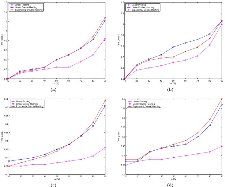
The first set of experiments, shown in Figure 1, is the same as those that were used to create the results shown in Table 1. Specifically, keys were generated ac-cording to the uniform distribution, andα·mdata ele-ments with these keys were stored in an initially empty hash table of size m= 400,009. On each machine con-figuration, 10 independent experiments were conducted, and the average of these was taken in order to create the results. Figure 1 shows the results for the four machine configurations when 8-byte data records were used. From Table 1 we know that the average num-ber of probes is fairly similar for all of the hash func-tions tested in this set of experiments. Furthermore, Table 1 showed that the average number of probes is relatively small, even at high load factors. Note in Fig-ure 1 that for this particular combination of data record size and hash table size, linear probing gains an advan-tage over the double hashing algorithms on each of the machine configurations tested, and that on three of the four configurations the advantage grows with increasing load factor. It is worth noting that in configuration 2 shown in Figure 1 (b), which is the Sun system with 8 MB of L2 cache, the advantage of linear probing is smaller, as one would expect. This particular set of ex-periments, involving the uniform distribution and small data records, is the only case we were able to construct where linear probing consistently outperformed double hashing over all load factors in terms of the actual time
10 20 30 40 50 60 70 80 90 0.5 0.6 0.7 0.8 0.9 1 1.1 1.2 1.3 α (%) Time ( µ sec.) Linear Probing Linear Double Hashing Exponential Double Hashing
(a) 10 20 30 40 50 60 70 80 90 0.5 0.6 0.7 0.8 0.9 1 1.1 1.2 α (%) Time ( µ sec.) Linear Probing Linear Double Hashing Exponential Double Hashing
(b) 10 20 30 40 50 60 70 80 90 0.3 0.35 0.4 0.45 0.5 0.55 0.6 0.65 0.7 0.75 α (%) Time ( µ sec.) Linear Probing Linear Double Hashing Exponential Double Hashing
(c) 10 20 30 40 50 60 70 80 90 0.3 0.35 0.4 0.45 0.5 0.55 0.6 0.65 0.7 α (%) Time ( µ sec.) Linear Probing Linear Double Hashing Exponential Double Hashing
(d)
Figure 1: The average insertion time for keys distributed according to the uniform distribution using a hash table of size m= 400,009, and 8-byte data records. Parts (a)–(d) correspond to configurations 1–4, respectively.
taken to perform the dynamic dictionary operations. Note, however, that for most load factors the advantage is not very significant, particularly when the time scale is taken into account. Furthermore, if the size of the data record is increased to 256 bytes (and with m = 100,003), our experiments indicate that this advantage is lost, and for each machine configuration, there is little performance difference between linear probing and the suitably defined double hash functions.
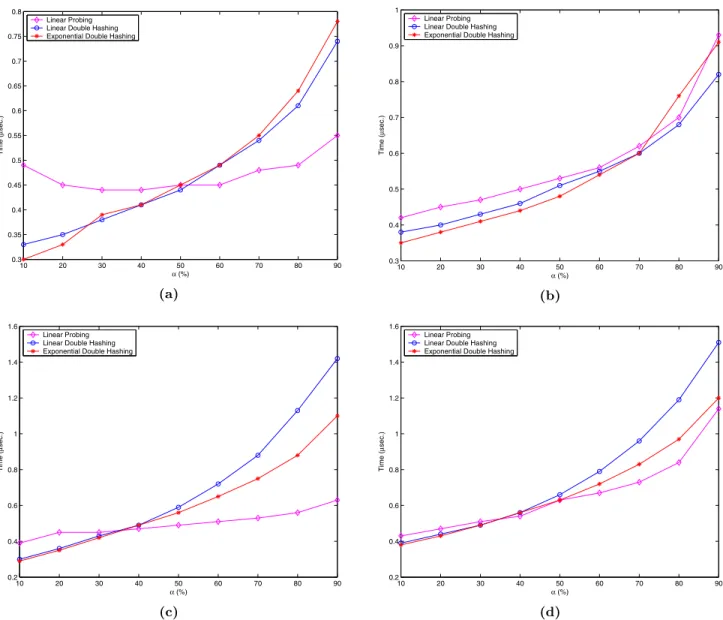
Next let us consider experiments that measure the cache effects related to the data shown previously in Table 3. Once again we tested the four different machine configurations on two different hash table/data record sizes, (1)m= 400,009 with 8-byte data records, and (2)
m = 100,003 with 256-byte data records. Each of the machine configurations produced fairly similar results, with machine configuration 2 slightly more favorable to double hashing due to its larger cache size. Figure 2 we present the results obtained on machine configuration 3. Once again, note that when the data record size is smaller (8 bytes) as in parts (a) and (c), linear probing with universal hashing does gain a slight advantage over the double hashing algorithms once the load factor exceeds approximately 50%. This is due to the larger number of cache hits per probe that occur in the case of linear probing. Notice, however, that in parts (b) and (d), where larger 256-byte records are used, double hashing tends to slightly outperform linear probing with universal hashing.
6 Conclusions.
In this paper we considered the performance of open address hashing algorithms when implemented on con-temporary computers. An emerging computing folklore contends that, in practice, linear probing is a better choice than double hashing, due to linear probing’s more effective use of cache memory. Specifically, although linear probing tends to produce longer probe sequences than double hashing, the fact that the percentage of cache hits per probe is higher in the case of linear prob-ing gives it an advantage in practice. Our experimen-tal analysis demonstrates that, given current technology and realistic data distributions, this belief is erroneous. Specifically, for many applications, where the data set largely fits in cache memory, there is never an advan-tage to linear probing, even when universal hashing is used. If a data set is large enough so that it does not easily fit into cache memory, then linear probing only has an advantage over suitably defined double hashing algorithms if the data record size is quite small. How-ever, it should be noted that one of the most common types of large data sets is the database, and records are typically quite large in databases.
The results provided in the open literature support-ing the superiority of linear probsupport-ing appear to be largely reliant on the assumption of a uniform data distribu-tion. The experimental analysis provided in this paper showed that indeed, assuming a uniform input distri-bution, it is possible for linear probing to consistently outperform double hashing. On the machine configura-tions we tested we were able to create some scenarios under which this occurred, but even in these cases, the advantage was slight. In particular, if the hash table was made large enough (so that the entire table would not fit in the cache), and the data records small enough (so that a large number of them would reside in cache), then by applying a uniform data distribution, linear probing could be made to outperform double hashing across all load factors. However, the performance gain was not very significant, particularly when this is con-trasted with the severe performance loss that accom-panies linear probing for nonuniform data distribution if the input distribution is not sufficiently randomized. In addition, it appears that in the case of the uniform distribution, the distribution itself is largely driving the performance. That is, by using a uniform distribution, there is a high probability that for any reasonably de-fined open address hash function, only one or two probes will be required to find an empty slot. Thus, the probing algorithm itself is largely unused. Therefore, as long as the uniformity of the data is preserved across the initial probes (this was not the case in one of the double hash-ing algorithms we considered), any open address hash function works about as good as any other, particularly when the load factor is not too large. Only the use of more realistic nonuniform data distributions causes the underlying characteristics of the probing algorithms to become evident. It was demonstrated that in this case double hashing, and in particular exponential double hashing, is far superior to linear probing. Indeed, even for very highly skewed input distributions the perfor-mance of exponential double hashing was little changed from that of the uniform input distribution case, while the running time for linear probing grows more signifi-cantly.
Although the effects of cache memory were explic-itly testing in our experiment, we believe that similar results would be obtained in testing the effects of virtual memory on open address hashing. In particular, for uni-form (or nearly uniuni-form) data distributions it should be possible to construct cases where linear probing slightly outperforms double hashing due to virtual memory ef-fects. However, this advantage would rapidly disappear when more realistic data distributions are applied.
10 20 30 40 50 60 70 80 90 0.3 0.35 0.4 0.45 0.5 0.55 0.6 0.65 0.7 0.75 0.8 α (%) Time ( µ sec.) Linear Probing Linear Double Hashing Exponential Double Hashing
(a) 10 20 30 40 50 60 70 80 90 0.3 0.4 0.5 0.6 0.7 0.8 0.9 1 α (%) Time ( µ sec.) Linear Probing Linear Double Hashing Exponential Double Hashing
(b) 10 20 30 40 50 60 70 80 90 0.2 0.4 0.6 0.8 1 1.2 1.4 1.6 α (%) Time ( µ sec.) Linear Probing Linear Double Hashing Exponential Double Hashing
(c) 10 20 30 40 50 60 70 80 90 0.2 0.4 0.6 0.8 1 1.2 1.4 1.6 α (%) Time ( µ sec.) Linear Probing Linear Double Hashing Exponential Double Hashing
(d)
Figure 2: The average insertion time for keys distributed according to the nonuniform distributions machine configuration 3. (a)N(m2,m4) withm= 400,009 and 8-byte data records,(b)N(m2,m4) withm= 100,003 and 256-byte data records, (c) c0.3 withm= 400,009 and 8-byte data records, and (d)c0.3 with m= 100,003 and
In summary, for the practitioner, the use of double hashing is clearly a good choice for general purpose use in dynamic dictionary applications that make use of open address hashing.
References
[1] Andrew Binstock. Hashing rehashed: Is RAM speed making your hashing less efficient? Dr. Dobb’s Journal, 4(2), April 1996.
[2] John R. Black, Jr., Charles U. Martel, and Hongbin Qi. Graph and hashing algorithms for modern archi-tectures: Design and performance. In Kurt Mehlhorn, editor,Proceedings of the 2nd Workshop on Algorithm Engineering (WAE’98), Saarbr¨ucken, Germany, Au-gust 1998.
[3] Andrei Broder and Michael Mitzenmacher. Using multiple hash functions to improve IP lookups. In
Proceedings of the Twentieth Annual Joint Conference of the IEEE Computer and Communications Societies (IEEE INFOCOM 2001), Anchorage, AK, April 2001. [4] Randal E. Bryant and David O’Hallaron. Computer Systems: A Programmer’s Perspective. Prentice-Hall, Inc., Upper Saddle River, NJ, 2003.
[5] J. Lawrence Carter and Mark N. Wegman. Universal classes of hash functions. Journal of Computer and System Sciences, 18(2):143–154, 1979.
[6] Trishul M. Chilimbi, James R. Larus, and Mark D. Hill. Tools for cache-conscious pointer structures. In
Proceedings of the 1999 ACM SIGPLAN Conference on Programming Language Design and Implementation, Atlanta, GA, May 1999.
[7] Thomas M. Cover and Joy A. Thomas. Elements of Information Theory. John Wiley & Sons, Inc., New York, 1991.
[8] The fifth DIMACS challenge–dictionary tests, Center for Discrete Mathematics & Theoretical Computer Science.
http://www.cs.amherst.edu/~ccm/challenge5/dicto/. [9] L. Guibas and E. Szemeredi. The analysis of double
hashing. Journal of Computer and Systems Sciences, 16:226–274, 1978.
[10] John L. Hennessy and David A. Patterson. Computer Architecture: A Quantitative Approach. Morgan Kauf-mann, San Francisco, 3rd edition, 2003.
[11] The King James Bible (KJV) download page. http://patriot.net/~bmcgin/kjvpage.html. [12] Donald E. Knuth. Searching and Sorting, volumeThe
Art of Computer Programming. Addison-Wesley, Reading, MA, 3rd edition, 1973.
[13] Anthony LaMarca and Richard E. Ladner. The influence of caches on the performance of heaps.
ACM Journal of Experimental Algorithmics,
1(4):www.jea.acm.org/1996/LaMarcaInfluence/, 1996.
[14] Anthony LaMarca and Richard E. Ladner. The in-fluence of caches on the performance of sorting. In
Proceedgins of the Eighth Annual ACM-SIAM Sympo-sium on Discrete Algorithms (SODA’97), pages 370– 379, New Orleans, LA, 1997.
[15] Alvin R. Lebeck and David A. Wood. Cache profiling and the SPEC benchmark: A case study. Computer, 27(10):15–26, 1994.
[16] G. Lueker and M. Molodowitch. More analysis of double hashing. In Proceedings of the 20th Annual ACM Symposium on the Theory of Computing, pages 354–359, 1988.
[17] Wenbin Luo and Gregory L. Heileman. Improved expo-nential hashing. IEICE Electronics Express, 1(7):150– 155, 2004.
[18] W. W. Peterson. Addressing for random access stor-age. IBM Journal of Research and Development, 1(2):130–146, 1957.
[19] Hongbin Qi and Charles U. Martel. Design and analysis of hashing algorithms with cache effects. http://theory.cs.ucdavis.edu/, 1998.
[20] Bradely J. Smith, Gregory L. Heileman, and Chaouki T. Abdallah. The exponential hash func-tion. ACM Journal of Experimental Algorithmics, 2(3):www.jea.acm.org/1997/SmithExponential/, 1997.
[21] Jeffrey D. Ullman. A note on the efficiency of hash functions. Journal of the ACM, 19(3):569–575, 1972. [22] Andrew C. Yao. Uniform hashing is optimal. Journal