Ariadna Quattoni1 [email protected] Universitat Polit`ecnica de Catalunya, Barcelona, Catalunya
Borja Balle1 [email protected]
McGill University, Montreal, QC, Canada
Xavier Carreras [email protected]
Universitat Polit`ecnica de Catalunya, Barcelona, Catalunya
Amir Globerson [email protected]
The Hebrew University of Jerusalem, Jerusalem, Israel
Abstract
We frame max-margin learning of latent variable structured prediction models as a convex opti-mization problem, making use of scoring func-tions computed by input-output observable oper-ator models. This learning problem can be ex-pressed as an optimization problem involving a low-rank Hankel matrix that represents the input-output operator model. The direct outcome of our work is a new spectral regularization method for max-margin structured prediction. Our exper-iments confirm that our proposed regularization framework leads to an effective way of control-ling the capacity of structured prediction models.
1. Introduction
Many important problems in machine learning can be framed as structured prediction tasks where the goal is to learn functions that map structured inputs to structured out-puts such as sequences or trees. This work focuses on se-quence tagging problems, where both inputs and outputs are sequences of equal length. This is an important task with applications in many domains where sequential data appears naturally, including speech and natural language processing. We note that although our contributions are de-scribed in a sequence tagging framework, ideas in this work can be generalized to other structured prediction settings. A standard approach to structured prediction is based on discriminative factorized linear models (Lafferty et al., Proceedings of the 31st International Conference on Machine Learning, Beijing, China, 2014. JMLR: W&CP volume 32. Copy-right 2014 by the author(s).
2001; Taskar et al.,2004), a direct generalization of lin-ear multiclass prediction to the setting of structured input-output pairs. The key idea is to break structures into parts and describe the relation between inputs and outputs us-ing a feature representation of each factor. The final scor-ing function for an input-output pair measures the compat-ibility of an outputywith an inputx. In factorized linear models the scoring function is assumed to be linear in the features that describe part-factored(x, y)pairs.
For sequence prediction, factors are usually associated with pairs of input-output sub-sequences, and the feature vec-tor of a complete sequence is obtained by adding the fea-tures of individual factors. With this approach, sequence prediction reduces to a linear multiclass problem with an exponential number of outputs. Prediction in this case re-quires solving an inference problem over the space of pos-sible outputs. Unlike with more complex models, in fac-torized linear models this inference problem can be effi-ciently solved. In addition, for appropriate loss functions, training these models can be formalized as a convex opti-mization problem (e.g., seeTaskar et al.,2004). In prac-tice, the caveat with these simple linear models is that in order to achieve good generalization performance, feature functions providing a good representation of the relevant input-output patterns for each problem domain need to be manually specified.
To address the limitations of factorized linear models, researchers have proposed to introduce latent variables and make the scoring function depend on those (Quattoni et al., 2004; Zhu et al., 2009; Wang & Mori, 2009; Yu & Joachims,2009; Girshick et al.,2011; Schwing et al., 2012). As their name indicates, these variables are not
1
observed at train or test time and their values need to be induced by the learning algorithm. The main idea is that models with latent variables have more freedom in explain-ing the relation between inputs and outputs, and can of-ten identify the relevant patterns in a given domain. How-ever, this increased expressivity comes at a price: the learn-ing problem becomes non-convex, and exact prediction in some of these models becomes intractable. In addition, as the number of parameters increases, choosing appropriate regularization strategies becomes essential to avoid overfit-ting.
Two popular approaches to structured prediction with la-tent variables are based on linear and log-linear models. The latent SVM algorithm (Yu & Joachims,2009) trains a linear model with latent variables by minimizing a regular-ized structured hinge loss under the assumption that pre-dictions are scored by maximizing over all possible assign-ments to the latent variables. Log-linear factorized models can be trained using a conditional logistic loss (Quattoni et al., 2004), or max-margin approaches (Wang & Mori, 2009). Scoring in these models can be done by maxi-mizing over all possible latent assignments, like with lin-ear models. However, when the loss function has a prob-abilistic interpretation (e.g. the conditional logistic loss), log-linear models can be normalized by a partition func-tion to induce a condifunc-tional distribufunc-tion over output struc-tures given an input structure and an assignment to the la-tent variables. A natural score in those cases is to consider the probability obtained by marginalizing over all possible latent assignments. Unfortunately, finding the output struc-ture that maximizes these marginalized scores is usually an intractable inference problem. Alternative approaches con-sider piecewise inference, where each factor of the output structure is predicted independently by marginalizing over all other factors (Quattoni et al.,2004). Overall, more pow-erful methods require solving more complex learning and prediction problems, and in most cases there is no clear match between the loss used at training and the inference rule used at prediction time.
In this paper we propose a model for sequence tagging with latent variables based on observable operator mod-els(OOM) (Jaeger,2000). These models, which include HMMs as a special case, provide a powerful modeling mechanism for scoring input-output sequences. Scoring functions computed by OOM naturally marginalize over the set of latent variables. This implies that finding maxi-mum score taggings involves an intractable inference prob-lem. To make the inference problem tractable we consider a piecewise loss function similar to segmented minimum Bayes-risk decoders used in speech recognition (Goel et al., 2004). We use this inference to define a loss function that explicitly considers the marginalized scores that will be used at prediction time, thus coupling the scores used for
prediction and learning. Then, by leveraging recent tech-niques in spectral learning of HMM and related models (Hsu et al., 2009; Bailly et al., 2009; Balle et al.,2011; Boots et al.,2011) and Hankel matrix completion (Balle & Mohri,2012; Bailly et al.,2013b;a), we give an efficient algorithm for learning OOM for sequence tagging with this loss function. Our algorithm combines a nuclear norm reg-ularized optimization with a spectral technique for recov-ering OOM from Hankel matrices. This provides a learn-ing algorithm without local minima, which, in contrast with other spectral algorithms, tries to agnostically fit a model to the data without making any explicit assumption about the distribution that generated it.
We report experiments where the proposed method is used to solve a word-to-phoneme transcription task. We show that spectral regularization is an effective way to control the capacity of the model, and that it outperforms standard
`2regularization. Furthermore, our method achieves
accu-racies similar to a feature-based Conditional Random Field for smaller training sets, and improves for larger training sets, without the need to design any features for the factors. 1.1. Notation
Bold letters are used to denote vectorsv∈Rdand matrices
M ∈ Rd1×d2. Given a matrixM we writekMk ∗ for its trace/nuclear norm, which is the sum of its singular values. We useM+to denote the Moore–Penrose pseudo-inverse
of M. Columns and rows of a matrix will sometimes be indexed by ordered setsI andJ. In this case we write
M∈RI×J to denote a matrix of size|I| × |J |with rows
indexed byIand columns indexed byJ.
LetX be a finite set. We use the standard notationX? to
denote the set of all finite sequences with elements in X. The empty sequence is denoted by . Given a sequence
x=x1· · ·xT ∈ XT of lengthTand indices1≤s≤t≤ T we usexs:tto denote the subsequencexs· · ·xt. Given
two sequencesu, v∈ X?we writew=u·v=uvfor their
concatenation;uandvare said to be a prefixes and suffixes ofwrespectively. Given two sets of sequencesP,S ⊆ X?
we writeP ·Sfor the set obtained by taking every sequence of the formuvwithu∈ Pandv∈ S.
2. Sequence Tagging with IO-OOM
2.1. Learning SettingLetXbe a set of input symbols andYa set of output sym-bols. Our goal is to learn a model forsequence taggingthat given an input sequence ofTsymbolsx∈ XT produces an
output sequencey ∈ YT. In this setting, a model is given
by ascoring functionF : (X × Y)?→
Rassigning a score F(x, y)to each pair of input and output strings. Given an input sequence x∈ XT the model predicts an output
se-quencey∈ YT by maximizing the score function: ˆ
y(x) = argmax
y∈YT
F(x, y) . (1)
The learning problem is specified via a class of possible scoring functionsFand a set of labeled training examples
S={(xi, yi)}m
i=1.
A widely used scoring function is the class of factorized linear models (e.g., seeLafferty et al.,2001;Collins,2002; Taskar et al.,2004). Assuming that some factor sizekand a feature function φthat maps factors to a vector repre-sentation are provided, the scoring function for sequence tagging is defined as:
F(x, y) = T
X
t=k+1
w·φ(x, yt−k:t) (2)
To measure the accuracy of tagging we are given a task lossfunction` : (Y × Y)? →
Rthat measures the
differ-ence `(y, y0)between two output sequences y, y0 ∈ YT.
For sequence tagging problems, a common choice for`is the Hamming distance that counts the number of symbols wherey andy0 differ. This can be regarded as the analog of the zero-one loss for the sequence prediction task. Minimizing the Hamming loss on the training data is com-putationally intractable for mostFof interest. The standard approach in these cases resorts to minimizing a surrogate lossLupper bounding the task loss. The learning problem is then: argmin F∈F m X i=1 L(xi, yi;F) +τ R(F) (3)
whereR(F)is a regularization term that controls the ca-pacity of the hypothesisF, and τ > 0is a regularization parameter. A common choice forLis thestructured hinge loss(Taskar et al.,2004):
Lhinge(x, y;F) = max
z [F(x, z)−F(x, y) +`(y, z)] .
2.2. Taggers with Latent Variables
The linearity ofF may be too restrictive in some settings. One mechanism for going beyond linearity is to introduce latent variables. We briefly review two such approaches below.
The main assumption behind latent variable predictors is the existence of a set of latent variablesH, each providing a possible explanation for the relation between an inputx
and an outputy. Given one possible explanation h∈ H, these models compute a vector of features: φ(x, y, h) ∈
RDdescribing the interactions betweenx,y, andh. As in
the linear methods, a weight vectorw is used to define a score onx, y, h: S(x, y, h) = T X t=k+1 w·φ(x, yt−k:k, ht−k:k) .
Given a score function S(x, y, h) there are two natural ways of obtaining a prediction.
Maximizing overh: Yu & Joachims(2009) suggested to obtain a prediction by maximizing overhand then overy. Namely, first define:F(x, y) = maxhS(x, y, h), and then predict via: y(x) = argmaxˆ yF(x, y), The loss of this predictor can be approximately minimized by using an ap-propriate variant of the structured hinge loss. This problem is known aslatent SVMand has shown impressive results in several applications, most notably machine vision ( Gir-shick et al.,2011). One major caveat is that the loss in this case is no longer convex, and a concave-convex alternating minimization procedure is used to find local minima. Summing Overh:An alternative inference procedure for
yis to consider the conditional distribution onygiven by:
p(y, h|x)∝exp (S(x, y, h)) .
Marginalizing this overhyields a score functionF(x, y)
(ignoring normalizing factors):
F(x, y) =X h
exp (S(x, y, h)) .
At this point there are two ways of predicting y. Either to further marginalizeF(x, y)to obtainF(x, yi)and take
argmaxyiF(x, yi). This is what is done in latent CRFs (Quattoni et al., 2004). An alternative, more consistent with the structured prediction methodology is to maximize
F(x, y)overy. However, as we argue later, this is a com-putationally hard task even for simple HMM like models. We note that it is also possible to consider intermedi-ate models that interpolintermedi-ate smoothly between the max
and sum inference criteria with soft-max type functions (Schwing et al.,2012).
Training of latent variable models always turns out to be non-convex because of the non-linear structure of the pre-diction. The goal of this work is to construct structured predictors that are as powerful as latent variable ones, but have convex training procedures, and tractable prediction functions. To achieve this, we turn to the powerful fam-ily of predictors corresponding to input-output observable operator models.
2.3. Input-Output Observable Operator Models We will now defineinput-output observable operator mod-els, which are a family of scoring functionsF(x, y)which
generalize the latent variable models above. An IO-OOM with inputX and outputY is a tupleA=hα,β,{Aa,b}i,
whereα,β ∈Rn andAa,b ∈ Rn×n for eacha ∈ X and b ∈ Y. The dimensionnis called the number of states of the model. Vectorsαandβare respectively the initial and final weights of the model. The matricesAa,b are known
as the observable operators of the model.
The IO-OOM can be used to define a score for eachx, y, h
combination as follows: S(x, y, h) =α(h0) T Y t=1 Axt,yt(ht−1, ht) ! β(hT) .
A score F(x, y) is then naturally defined by summation overh, and is given by the compact algebraic expression:
F(x, y) =X h
S(x, y, h) =α>Ax1,y1· · ·AxT,yTβ .
Prediction ofycan now be done as before by maximizing
F(x, y)overy.
We shall writeFAto denote the scoring function computed
byA. IO-OOM are a powerful formalism stemming from stochastic process models in control theory (Jaeger,1998; 2000), with tight relations to weighted automata and trans-ducers (Droste et al.,2009), and predictive state represen-tations (Littman et al.,2001).
To link the F(x, y)of IO-OOM to that of latent variable models in Section 2.2, note that if theφ(x, y, h)used in the latter uses the scope xi, yi, ht, ht−1 then it is exactly
captured by an IO-OOM. This is just a different way of saying that IO-OOM can compute the same functions as HMM. In fact it is well known that the class of functions computed by IO-OOM is a superset of those computed by HMMs (Jaeger,2000).
From now on we will take IO-OOM with arbitrary coeffi-cients as our class of hypothesis scoring functions. In the next section we show how to predict using these models, and in the sequel we focus on learning them from data. 2.4. Piecewise Prediction for IO-OOM
The first challenge to using IO-OOM is that of performing prediction, i.e. maximizingF(x, y)in (2.3). It turns out that this is an NP hard task (Lyngsø & Pedersen,2002) so that approximations are required.
A common approach to approximate the most likely output of IO-OOM is to use a piecewise version ofFfor scoring
k-grams ofyindependently and then obtain an output that maximizes the sum of those scores using a dynamic pro-gramming algorithm (Goel et al.,2004). More formally, suppose we are given a scoring functionF, an orderk≥1, and sequencesx, yof lengthT ≥k. Then one can consider
the following approximate inference rule
ˆ yk(x) = argmax y T X t=k+1 F(xt−k:t, yt−k:t) = argmax y Fk(x, y) . (4)
The above only considers dependencies between input and output k-gram, and their additive effect. A more general version of this can be obtained by looking atl-grams for all
l≤k: ˆ y[k](x) = argmax y k X l=1 T X t=l+1 F(xt−l:t, yt−l:t) = argmax y F[k](x, y) .
Using these piecewise approximations of F we can de-fine tractable relaxations of the structured hinge loss for IO-OOM. In particular, we define the Viterbi-hinge
losses given by Lk(x, y;F) = Lhinge(x, y;Fk) and
L[k](x, y;F) =Lhinge(x, y;F[k]). For sequences of length T these loss functions can be computed in timeO(T|Y|k)
using Viterbi’s algorithm.2
Now that we have a loss that we can evaluate for the class of IO-OOM, we can ask what is a natural regularizer for this class. In this case, an obvious choice is the number of states of an IO-OOM, which we denote by|A|. UsingFto denote the class of all scoring functions computed by IO-OOM, we would now like to learn a sequence tagger of the formFAby solving the optimization problem
argmin A∈F m X i=1 L(xi, yi;FA) +τ|A| , (5)
withL=LkorL=L[k]for some given orderk.
In general this turns out to be a hard problem because even ifLcan be efficiently evaluated for small values ofk, when
k≥2the dependence ofL(x, y;FA)on the parameters of Ais non-convex. In particular, assuming a fixed number of states forA, we see that the expression forL(x, y;FA)
in-volves terms of the formα>Axt,yt· · ·Axt+l,yt+lβ, which are polynomials of degreel+ 3in the parameters ofA =
hα,β,{Aa,b}i, and are non-convex inA. Our agenda for
the following sections is to obtain an approximate solu-tion for this problem by relaxing the objective funcsolu-tion and splitting the learning procedure into two tractable subprob-lems.
3. A Spectral Algorithm for Learning
Max-Margin IO-OOM
To address the non-convexity of (5) we first observe that the loss is convex in the actualvaluesofFA.3 This means that if we represent the optimization variable as a list of values on(X × Y)≤kgiven by some functionF instead of
an IO-OOMA, the optimization problem becomes convex. However, this poses three key challenges:
• The values ofF should correspond to valid IO-OOM. • The regularizer|A|should correspond to the rank of
the IO-OOM described byF.
• Given anFthat corresponds to an IO-OOM, how can one recover the matricesAthat define it?
In what follows, we show that all these difficulties can be addressed, and that optimizing with respect to the values of
FAinstead of the parameters ofAyields an optimization
problem over a set of Hankel matrices. Then, by leveraging recent techniques on spectral learning of OOM via Hankel matrix completion, we can recover an IO-OOM from the solution of this optimization problem with a simple SVD computation.
3.1. IO-OOM and Hankel Matrices
To explain our approach we first introduce the concept of Hankel matrices ofF. These matrices provide an algebraic formalism to study the problem of recovering an IO-OOM from evaluations of its scoring functionF : (X ×Y)?→
R.
LetP,S ⊆(X ×Y)?be sets of input-output sequences. We
call the pairs(u, w)∈ P prefixes and the pairs(v, z)∈ S suffixes. A Hankel matrixH∈RP×S forFover the basis
(P,S)is obtained by taking the entries ofHto be
H((u, w),(v, z)) =F(uv, wz) . (6) A well-known theorem (Sch¨utzenberger,1961;Carlyle & Paz,1971; Fliess,1974) states that a functionF : (X × Y)? →
R can be realized by an IO-OOM withn states
if and only if, for very possible basis the corresponding Hankel matrixH of F has rank at mostn. A construc-tive version of this theorem lies at the very heart of recent spectral algorithms for learning HMM (Hsu et al.,2009), weighted automata (Bailly et al., 2009; Balle & Mohri, 2012), weighted transducers (Balle et al.,2011), and other families of recursively defined functions over sequences with discrete observations (Siddiqi et al.,2010;Boots et al., 2011).
When applied to IO-OOM, the spectral algorithm works as follows. Let us assume thatFcan be realized by a minimal
3Specifically, it is piecewise linear in those.
IO-OOM withnstates and that we are given a basis(P,S)
such that the corresponding Hankel matrix ofF, which we denote byH,, has rankn. Suppose we are also given, for
each(a, b)∈ X ×Y, the Hankel matrixHa,b∈RP×Swith
entries Ha,b((u, w),(v, z)) = F(uav, wbz), and vectors
hP ∈RP andhS ∈RS with entries given byhP(u, w) =
F(u, w)andhS(v, z) =F(v, z). Then the following pro-cedure recovers an IO-OOMA=hα,β,{Aa,b}isuch that FA =F: first, take the reduced SVD ofH,=UΣV>;
and then, build A by taking Aa,b = (H,V)+Ha,bV,
α>=h>
PV, andβ= (H,V)+hS.
A fundamental property of this spectral algorithm is its ro-bustness to noise. In particular, when the entries in these Hankel matrices are noisy estimates of values computed by an IO-OOM, the algorithm will produce a model which is close to the true model in terms of`1distance. The
paradig-matic example of this approach is the algorithm for learning HMM of (Hsu et al.,2009), where the noisy Hankel matri-ces come from empirical estimates of observation proba-bilities. A different approach, which is the one we pursue here, is to obtain an approximate Hankel matrix by solving a matrix completion problem with a loss function defined in terms of the task loss (Balle & Mohri,2012;Bailly et al., 2013b;a). The next section shows how to apply this method to max-margin learning of IO-OOM.
3.2. Max-Margin Completion of Hankel Matrices The discussion in the previous section implies that the set ofF values for an IO-OOM of ranknis equivalent to the set of Hankel matrices of rankn. Thus, the optimization of (5) can be equivalently performed on Hankel matrices with rank regularization. We next elaborate on this problem, and address the difficulty of optimizing the rank.
To obtain a Hankel matrix completion problem from (5) we proceed as follows. First we parameterize an IO-OOM via its corresponding Hankel matrixH(P,S)(over some fixed
basis(P,S)) instead of the originalAmatrices representa-tion. Next we change the regularizer: instead of the number of states of an IO-OOM, the Hankel/IO-OOM equivalence theorem says that we can take the rank of the Hankel matrix as a regularizer that directly controls the number of states of the learned IO-OOM. This yields the following optimiza-tion problem argmin H∈H(P,S) m X i=1 L(xi, yi;H) +τrank(H) , (7)
which by the relation between IO-OOM and Hankel matri-ces is almost equivalent to (5), with the only difference that now the search is conducted over the class of all IO-OOM that can be recovered from Hankel matrices inH(P,S).
The choice of a right basis(P,S)is essential if we want to be able to use information from all training examples,
and also guarantee that we can recover an IO-OOM from the learned Hankel matrix. When using lossL[k], the first
point requires that we have∪k
l=1gramsl(S)⊆ P ·S, where gramsl(S)is the set of all input-outputl-grams observed in
the training sampleS. Similarly, forL=Lkwe need a
ba-sis such that gramsk(S) ⊆ P · S. To recover operators forFusing the spectral method, we will retrieve theH,,
Ha,b,hP0 andhS0 defined in Section3.1as sub-blocks of the learned Hankel matrix; note that these sub-blocks will correspond to a basis(P0,S0)smaller than the(P,S)used in (7) (see (Balle & Mohri,2012) for further details). One way to guarantee that H contains the right sub-blocks is by choosing an initial basis(P0,S0)with(, )∈ P0∩ S0, and then take P = P0·(X0 × Y0) andS = S0, where X0 = X ∪ {}andY0 = Y ∪ {}. Note that (6) implies that entries in Hankel matrices corresponding to pairs of prefixes and suffixes that yield the same input-output se-quence must have the same value. Taking a larger basis implies that more constraints will need to be satisfied in the matrix search space considered by the completion algo-rithm. Therefore, a good strategy to keep the optimization as simple as possible is to choose the minimal basis satis-fying the constraints outlined above.
The last step needed to obtain a convex optimization is to relax the regularization term in (7), replacing it with the nu-clear norm of the Hankel matrix. This last step is a usual approach in matrix completion problems, and can be justi-fied by observing that because the nuclear norm of a matrix is precisely the `1 norm of its singular values,
minimiz-ing the nuclear norm yields (approximately) low rank ma-trices in the same way that`1regularization yields sparse
vectors (Cand`es & Recht,2009). Therefore, assuming the basis(P,S)is given, we can put together the ingredients described so far to get the following optimization problem over a space of Hankel matrices:
ˆ HS ∈ argmin H∈H(P,S) m X i=1 L(xi, yi;H) +τkHk∗ . (8)
One last observation is that in the caseL =Lk, it is pos-sible to choose the basis in a way that the space of Hankel matrices in (8) contains no equality constraints. This can be interesting if we are willing to give up on the ability to recover an IO-OOM from the learned matrix, and use the values in HˆS for predicting using the inference rule (4).
From an algorithmic point of view, this can be interpreted as taking a trade-off between memory and time for predict-ing with the learned model. Obtainpredict-ing the IO-OOM op-erators fromHˆS yields a high rate of compression, at the
price of needing several matrix multiplications every time a score needs to be computed. On the other hand, one can store the whole matrixHˆS and treat it as cached scores for
each possible input-outputk-gram.
4. Optimization Details
In this section we describe the details of an optimization algorithm for solving problem8. For simplicity we focus on the settingL=Lk with a basis(P,S)where the Han-kel matrices inH(P,S)contain no equality constraints. It
is easy to extend the algorithm for basis with equality con-straints by adding an extra projection step.
Recall that our goal is to minimize the following function:
g(H) = m
X
i=1
Lk(xi, yi;H) +τkHk∗ ,
To simplify notation we denote the overall loss byLS(H)
so thatg(H) =LS(H) +τkHk∗.
Since both the loss and the trace norm are convex it turns out thatg(H)is convex, albeit non differentiable. In recent years, many algorithms have been proposed for optimizing trace norm regularized problems (e.g., seeJaggi & Sulovsk, 2010;Shalev-Shwartz et al.,2011;Ji & Ye,2009). Some of these methods only apply to smooth losses and are thus not applicable here.4 Furthermore, some of these require solving optimization problems that are costly in our setting (e.g., backward fitting as inShalev-Shwartz et al.,2011). Here we use a simple optimization scheme known as For-ward BackFor-ward Splitting, or FOBOS (Duchi & Singer, 2009). FOBOS is similar to proximal gradient, with the exception that it linearizes the loss part ofg(H)(and not the regularizer). It corresponds to the following repeated updates on Ht. First, take a step in the direction of the
subgradient of the loss (ignoring the trace norm):
Ht+0.5=Ht−ηt
∂LS(Ht) ∂H
whereηt= √ctis a step size and
∂LS(Ht)
∂H is a sub gradient
of the loss atHt. This is easily evaluated for the hinge loss
we consider, and involves finding the argmax of the hinge loss. In the second step, find anHthat is close toHt+0.5
but with a trace norm penalty:
Ht+1= argmin
H
kHt+0.5−Hk22+ηtτkHk∗ .
This step can be solved via SVD thresholding (see Cai et al., 2010) as follows. Use SVD to write Ht+1 as
Ht+1 = UΣV> with Σ a diagonal matrix and U,V
orthogonal matrices. Denote by σi the ith element on the diagonal of Σ. Define a new matrix Σ¯ with diago-nal elementsσi¯ = max [σi−ηtτ,0]. The update is then:
Ht+1 = UΣV¯ >. Each update requires calculating an
4
Note however that it is possible to smooth the loss using standard methods (Nesterov,2005) and then use algorithms for smooth objectives.
Algorithm 1FOBOS minimization ofLS(H) +τkHk∗. InitializeH0= 0 whilet <MaxIterdo SetGtto a subgradient ofLS(H)atHt. Setηt=√c t. SetHt+0.5=Ht−ηtGt.
Calculate the SVD ofHt+0.5asHt+0.5=UΣV>.
Define a diagonal matrix Σ¯ such that σi¯ = max [σi−ηtτ,0].
SetHt+1=UΣV¯ >. end while
SVD ofH. For the problem sizes we considered this was fairly fast to compute. It can be further sped up by using the fact that only leading singular vectors are required and us-ing methods that only calculate these. FurthermoreHt+0.5
is typically a low rank plus sparse matrix, which can be used for further speedups.
It can be shown (Duchi & Singer,2009) that FOBOS con-verges to the global optimum ofg(H)at a rate ofO(ε−2). Although rates ofO(ε−1)are possible via accelerated gra-dient (Ji & Ye,2009), we find it is sufficient for the appli-cations we consider.
5. Experimental Results
In this section we present experimental results on a text-to-phonemes task. We compare the max-margin sequence tagging method with spectral regularization to several al-ternative methods.
We used the “Nettalk” dataset (a.k.a. the Connection-ist Bench), available from the UCI repository (Sejnowski & Rosenberg, 1987). The data consists of 20,008 En-glish words (formed with 26 letters) paired with a phonetic representation (using 51 phoneme symbols). For exam-ple, appleis paired with@p-L-andhippopotamus
withhIp-xpatxmxs. Input-output sequence pairs in the data have one-to-one monotonic alignments (using a spe-cial symbol “-” to represent many-to-one letter to phoneme associations, as shown in the examples), which results in paired sequences of equal length. We consider the task of predicting the phoneme sequence given an input word. We use Hamming accuracy to compare the performance of different methods. We randomly divided the dataset into 15,000 training sequences, 1,034 development sequences and 3,974 test sequences. We created 6 training sets of in-creasing size to obtain a learning curve.
We trained several types of sequence tagging models that exploit trigram factorizations, and for all of them we used the Viterbi algorithm as inference routine5. We compare 5The number of output trigrams is a constant of all sequence
the following models:
• IO-OOM with Spectral Max-Margin: To set the basis of the Hankel matrix, we use all observed bi-symbols for prefixes and for suffixes. In this config-uration the matrix HˆS we obtain has values for all
input-output trigrams, and we can directly use it to tag sequences. The parameters of the method are the reg-ularization constantτ, an initial learning ratecand the number of iterations.
• IO-OOM with Unregularized Max-Margin: This method drops the spectral regularizer. It is equivalent to settingτ= 0.
• IO-OOM with L2 Max-Margin: This method re-places the spectral regularizer with a standard `2
penalty on the coefficients of the Hankel matrix; that is, the trace norm regularizerkHk∗is replaced with a Frobenius norm regularizerkHkF.
• Spectral IO-HMM:The standard spectral method for HMM applied to joint sequences (Hsu et al., 2009), which estimates Hankel matrices directly from empir-ical counts on the training sample. We also tried the spectral method for conditional IO models by (Balle et al.,2011) but we obtained development accuracies significantly lower than other methods, around 70%. • Latent SVM: The latent SVM by (Yu & Joachims,
2009), which follows a Max-Max approach and at-tempts to solve a non-convex problem. We used their implementation adapted to sequence tagging, using the same features as an IO-OOM seen as a log-linear model. We could only find configurations that ob-tained very moderate training accuracies, at the level of 60%.
• CRF and Averaged Perceptron:A standard feature-based trigram Conditional Random Field tagger (CRF), that represents input-output trigrams using sub-pattern features. We used the code by (Collins et al.,2008), which implements structured prediction learning algorithms and tagging models that obtain state-of-the-art accuracies in part-of-speech tagging. As features, it exploits each bi-symbol with various combinations of the input context, and with various combinations of the the output context in the trigram. taggers, and considering all possible output trigrams for this data (i.e. 513) is impractical. Instead of pairing each input symbol with each output symbol, for each training set we restricted to the set of bi-symbols observed in the training data. For the largest training set, input symbols are paired with 2 to 18 output sym-bols. This dramatically reduces the number of possible trigrams, and has very low impact in prediction accuracy. This strategy is common in tagging tasks such as part-of-speech tagging.
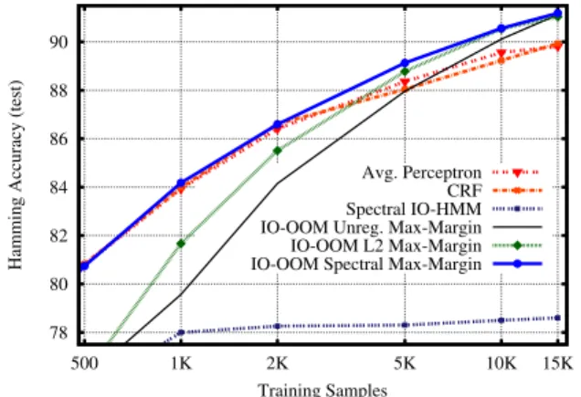
78 80 82 84 86 88 90 500 1K 2K 5K 10K 15K
Hamming Accuracy (test)
Training Samples
Avg. Perceptron CRF Spectral IO-HMM IO-OOM Unreg. Max-Margin IO-OOM L2 Max-Margin IO-OOM Spectral Max-Margin
Figure 1.Learning curve for various methods. We plot test accu-racy with respect to size of the training set.
84.5 85 85.5 86 86.5 87 87.5
Hamming Accuracy (development)
IO-OOM Unreg. Max-Margin IO-OOM L2 Max-Margin IO-OOM Spectral Max-Margin
Figure 2.Regularization path for Spectral and L2 regularization, using a training set of 2,000 samples. We plot development accu-racy with respect to values of the regularization constantτ. The range of relevantτvalues of each model has been normalized.
For parameter estimation we tried the log-linear loss (i.e. CRF), structured max-margin loss, and averaged Perceptron. All methods performed similarly. We trained all models on training sets of different sizes, trying a wide range of regularization constants when ap-plicable. We used accuracy on development sequences to pick the best configuration. Figure1 plots test accuracies for each method. We can see that spectral regularization largely improves over the unregularized model: in the first points of the curve the spectral approach requires half of the training samples to get to the same accuracy as the un-regularized one. Comparing regularizers, the spectral one shows a better curve than the`2, especially in the first part
of the curve. We attribute this to the ability of the regu-larizer to factor input-output trigrams using a hidden rep-resentation. As the number of samples increases, the non-factored representation of trigrams is effective and the two regularizers perform similarly. Figure2presents the regu-larization path for the spectral and`2regularizers for 2,000
training samples. At their best configurations in develop-ment, the Spectral improves 2.2 points over the
unregular-ized model, while the`2improves 1.1 points.
We can observe that in the first part of the curve the spec-tral regularization performs very similarly to feature-based models trained with Perceptron or CRF. This suggests that the factorization obtains a representation that is as effective as manually-specified sub-pattern features. As the number of examples increases, the full trigram parameters become useful and the spectral regularizer leverages them, while the feature-based models stop improving. In all, the spec-tral regularization technique seems to perform the best in any of the empirical scenarios.
6. Conclusion
The central contribution of this paper is to derive a con-vex formulation for max-margin structured prediction with latent variables and max-sum prediction rules. The main outcome of our work is a new regularization approach, inspired by spectral techniques, which is specifically de-signed for structured prediction tasks. This means that, in-stead of designing the features of a factorized linear model, we can consider rich function spaces and implicitly induce features via proper regularization. Our experiments con-firm that the proposed regularization framework leads to an effective way of controlling the capacity of structured pre-diction models.
Spectral methods for latent variable models require a single SVD calculation and are non-iterative in nature. While this is an attractive feature, it is justified only in the case where data is indeed generated from the assumed latent variable model (e.g., inHsu et al.,2009, it is assumed that data is generated from an HMM). In our formalism no such as-sumptions are made. The latent variable construct is only a mechanism for generating a prediction function. Thus the Hankel matrix we consider does not correspond to ob-served statistics of some assumed model but rather corre-sponds to unknown parameters of a prediction function. Our work suggests that core ideas behind spectral learning can have wide applicability to structured prediction. Our results can be generalized to other loss functions as long as they have surrogate piecewise approximations.
Acknowledgments
We thank the reviewers for their helpful comments. This work was supported by projects XLike (FP7-288342), ERA-Net CHISTERA VISEN, TACARDI (TIN2012-38523-C02-00) and by the ISF Centers of Excellence (grant 1789/11). Xavier Carreras was supported by the Ram´on y Cajal program of the Spanish Government (RYC-2008-02223). Borja Balle received support from NSERC and the James McGill Research Fund.
References
Bailly, R., Denis, F., and Ralaivola, L. Grammatical inference as a principal component analysis problem.ICML, 2009. Bailly, R., Carreras, X., Luque, F., and Quattoni, A.
Unsuper-vised spectral learning of WCFG as low-rank matrix comple-tion.EMNLP, 2013a.
Bailly, R., Carreras, X., and Quattoni, A. Unsupervised spectral learning of finite state transducers. InNIPS, 2013b.
Balle, B. and Mohri, M. Spectral learning of general weighted automata via constrained matrix completion.NIPS, 2012. Balle, B., Quattoni, A., and Carreras, X. A spectral learning
algo-rithm for finite state transducers.ECML, 2011.
Boots, B., Siddiqi, S., and Gordon, G. Closing the learning plan-ning loop with predictive state representations. International Journal of Robotics Research, 2011.
Cai, J-F., Cand`es, E.J., and Shen, Z. A singular value thresholding algorithm for matrix completion. SIAM Journal on Optimiza-tion, 2010.
Cand`es, E.J. and Recht, B. Exact matrix completion via con-vex optimization.Foundations of Computational mathematics, 2009.
Carlyle, J. W. and Paz, A. Realizations by stochastic finite au-tomata.Journal of Computer Systems Science, 1971.
Collins, M. Discriminative training methods for hidden markov models: theory and experiments with perceptron algorithms. In Proceedings of the conference on Empirical methods in natu-ral language processing, pp. 1–8, Morristown, NJ, USA, 2002. Association for Computational Linguistics.
Collins, M., Globerson, A., Koo, T., Carreras, X., and Bartlett, P. Exponentiated Gradient Algorithms for Conditional Random Fields and Max-Margin Markov Networks.Journal of Machine Learning Research, 9(2):1775–1822, 2008.
Droste, M., Kuich, W., and Vogler, H. Handbook of weighted automata. Springer, 2009.
Duchi, J. and Singer, Y. Efficient online and batch learning using forward backward splitting.The Journal of Machine Learning Research, 2009.
Fliess, M. Matrices de Hankel. Journal de Math´ematiques Pures et Appliqu´ees, 1974.
Girshick, Ross B., Felzenszwalb, Pedro F., and Mcallester, David. Object detection with grammar models. InIn NIPS, 2011. Goel, V., Kumar, S., and Byrne, W. Segmental minimum
bayes-risk decoding for automatic speech recognition. Speech and Audio Processing, IEEE Transactions on, 2004.
Hsu, D., Kakade, S. M., and Zhang, T. A spectral algorithm for learning hidden Markov models.COLT, 2009.
Jaeger, H. Discrete-time, discrete-valued observable operator models: A tutorial. Technical report, GMD Report 42, German National Research Center for Information Technology, 1998. Jaeger, H. Observable operator models for discrete stochastic time
series.Neural Computation, 2000.
Jaggi, M. and Sulovsk, M. A simple algorithm for nuclear norm regularized problems. InICML, 2010.
Ji, S. and Ye, J. An accelerated gradient method for trace norm minimization. InICML, 2009.
Lafferty, J., McCallum, A., and Pereira, F. Conditional random fields: Probabilistic models for segmenting and labeling se-quence data. InProceedings of the 18th International Confer-ence on Machine Learning, pp. 282–289. Morgan Kaufmann, San Francisco, CA, 2001.
Littman, M. L., Sutton, R. S., and Singh, S. Predictive represen-tations of state. InNIPS, 2001.
Lyngsø, R. B. and Pedersen, C. N. S. The consensus string prob-lem and the complexity of comparing hidden markov models. J. Comput. Syst. Sci., 2002.
Nesterov, Yu. Smooth minimization of non-smooth functions. Mathematical Programming, 103(1):127–152, 2005.
Quattoni, A., Collins, M., and Darrell, T. Conditional random fields for object recognition. InIn NIPS, pp. 1097–1104. MIT Press, 2004.
Sch¨utzenberger, M. P. On the definition of a family of automata. Information and Control, 1961.
Schwing, A.G., Hazan, T., Pollefeys, M., and Urtasun, R. Ef-ficient structured prediction with latent variables for general graphical models. InICML, 2012.
Sejnowski, T.J. and Rosenberg, C.R. Parallel networks that learn to pronounce english text.Complex Systems, 1:145–168, 1987. Shalev-Shwartz, S., Gonen, A., and Shamir, O. Large-scale con-vex minimization with a low-rank constraint. InICML, 2011. Siddiqi, S.M., Boots, B., and Gordon, G.J. Reduced-rank hidden
Markov models.International Conference on Artificial Intelli-gence and Statistics (AISTATS), 2010.
Taskar, B., Guestrin, C., and Koller, D. Max margin Markov net-works. In Thrun, S., Saul, L., and Sch¨olkopf, B. (eds.), Ad-vances in Neural Information Processing Systems 16, pp. 25– 32. MIT Press, Cambridge, MA, 2004.
Wang, Y. and Mori, G. Max-margin hidden conditional random fields for human action recognition. InCVPR, 2009.
Yu, C-N. and Joachims, T. Learning structural svms with latent variables. InICML, 2009.
Zhu, Jun, Xing, Eric P., and Zhang, Bo. Partially observed maxi-mum entropy discrimination markov networks. InProc. NIPS, 2009.