Parametric frailty and shared frailty survival models

(1)

The Stata Journal

Editor

H. Joseph Newton Department of Statistics Texas A & M University College Station, Texas 77843 979-845-3142 979-845-3144 FAX [email protected] Executive Editor Nicholas J. Cox Department of Geography University of Durham South Road

Durham City DH1 3LE United Kingdom [email protected] Associate Editors Christopher Baum Boston College Rino Bellocco Karolinska Institutet David Clayton

Cambridge Inst. for Medical Research Charles Franklin

University of Wisconsin, Madison Joanne M. Garrett

University of North Carolina Allan Gregory

Queens University James Hardin

Texas A&M University Stephen Jenkins

University of Essex Jens Lauritsen

Odense University Hospital

Stanley Lemeshow Ohio State University J. Scott Long

Indiana University Thomas Lumley

University of Washington, Seattle Marcello Pagano

Harvard School of Public Health Sophia Rabe-Hesketh

Inst. of Psychiatry, King’s College London J. Patrick Royston

MRC Clinical Trials Unit, London Philip Ryan

University of Adelaide Jeroen Weesie

Utrecht University Jeﬀrey Wooldridge

Michigan State University

Copyright Statement:The Stata Journal and the contents of the supporting files (programs, datasets, and help files) are copyright cby Stata Corporation. The contents of the supporting files (programs, datasets, and help files) may be copied or reproduced by any means whatsoever, in whole or in part, as long as any copy or reproduction includes attribution to both (1) the author and (2) the Stata Journal.

The articles appearing in the Stata Journal may be copied or reproduced as printed copies, in whole or in part, as long as any copy or reproduction includes attribution to both (1) the author and (2) the Stata Journal. Written permission must be obtain ed from Stata Corporation if you wish to make electronic copies of the insertions. This precludes placing electronic copies of the Stata Journal, in whole or in part, on publically accessible web sites, fileservers, or other locations where the copy may be accessed by anyone other than the subscriber.

Users of any of the software, ideas, data, or other materials published in the Stata Journal or the supporting files understand that such use is made without warranty of any kind, by either the Stata Journal, the author, or Stata Corporation. In particular, there is no warranty of fitness of purpose or merchantability, nor for special, incidental, or consequential damages such as loss of profits. The purpose of the Stata Journal is to promote free communication among Stata users.

TheStata Technical Journal, electronic version (ISSN 1536-8734) is a publication of Stata Press, and Stata is a registered trademark of Stata Corporation.

(2)

2

Parametric frailty and shared frailty survival

models

Roberto G. Gutierrez Stata Corporation

Abstract. Frailty models are the survival data analog to regression models, which account for heterogeneity and random effects. A frailty is a latent multiplicative ef-fect on the hazard function and is assumed to have unit mean and varianceθ, which is estimated along with the other model parameters. A frailty model is an hetero-geneity model where the frailties are assumed to be individual- or spell-specific. A shared frailty model is a random effects model where the frailties are common (or shared) among groups of individuals or spells and are randomly distributed across groups. Parametric frailty models were made available in Stata with the release of Stata 7, while parametric shared frailty models were made available in a recent series of updates. This article serves as a primer to those fitting parametric frailty models in Stata via thestreg command. Frailty models are compared to shared frailty models, and both are shown to be equivalent in certain situations. The user-specified form of the distribution of the frailties (whether gamma or inverse Gaussian) is shown to subtly affect the interpretation of the results. Methods for obtaining predictions that are either conditional or unconditional on the frailty are discussed. An example that analyzes the time to recurrence of infection after catheter insertion in kidney patients is studied.

Keywords: st0006, parametric survival analysis, frailty, random eﬀects, overdis-persion, heterogeneity

1 Introduction

Parametric survival models are regression models in which the distribution of the re-sponse is chosen to be consistent with what one would see if the rere-sponse is time-to-failure. In particular, the distribution of the response should have positive support. Examples of such distributions are the exponential, Weibull, log-normal, log-logistic, Gompertz, and the generalized gamma, among others. Survival models also diﬀer from standard regression models in their ability to account for censoring and truncation.

For purposes of interpretability, the distribution of time-to-failure is oftentimes char-acterized by the hazard function, which is the ratio of the probability density function to one minus the cumulative density function. Hazard functions also provide a conve-nient means to adjust for regressors, either by assuming that the covariates serve to multiplicatively shift the hazard function (proportional hazards) or by assuming that the covariates serve to accelerate or decelerate the eﬀect of time (accelerated failure time).

c

(3)

A frailty model is a generalization of a survival regression model. In addition to the observed regressors, a frailty model also accounts for the presence of a latent multiplica-tive effect on the hazard function. This effect, or frailty, is not directly estimated from the data, but instead is assumed to have unit mean and finite variance, which is esti-mated. In cases where the frailty is greater than one, subjects experience an increased hazard (or risk) of failure and are said to be more frail than their cohorts. In this way, frailty models can provide a useful alternative to a standard survival model when the standard model fails to adequately account for all the variability in the observed failure times.

Frailty models come in two flavors. Thefrailty modelis used with univariate data and is used to model heterogeneity among individuals, analogous to how negative binomial regression generalizes Poisson regression, since the negative binomial may be derived from a Poisson model by introducing a latent gamma-distributed effect. The shared frailty model is used with multivariate survival data where the unobserved frailty is shared among groups of individuals, and thus a shared frailty model may be thought of as a random effects model for survival data. In this way, a shared frailty model would be analogous to how a Poisson random effects model (estimated viaxtpois) generalizes the standard Poisson model.

Frailty models for univariate data have long been used to account for heterogeneous times-to-failure. The term frailty was first suggested by Vaupel et al. (1979) in the context of mortality studies, andLancaster(1979) incorporated the frailty concept into a study of duration of unemployment. Hougaard(1984) discusses the ramifications of the assumed distribution of the frailty, whether gamma or inverse Gaussian. In particular, for the gamma frailty distribution the relative variability of the frailties among survivors is shown to remain constant, whereas for the inverse Gaussian the relative variability decreases with age, making the population of survivors more homogeneous with the passage of time. Hougaard(1986b) considers the positive stable family of distributions for the frailty, not available for estimation in current Stata. The positive stable family is appealing under this family because if individual hazards are proportional, then so are the population hazards. In general, however, the relative shapes of the individual and population (unconditional on the frailty) hazard functions can differ extensively due to thefrailty effect— the more frail individuals tend to fail earlier, leaving a more homogeneous population of survivors.

Shared frailty models for multivariate data have the added appeal that the frailty can be used to model intragroup correlation. Early considerations of these models can be found inClayton(1978) andClayton and Cuzick(1985), and much of the development in this area stems from the extension of methods used to measure correlation in bivari-ate survival data with arbitrary individual hazard functions (including Cox models).

Hougaard(1986a) examines the shared frailty model with Weibull individual hazards,

andWhitmore and Lee (1991) look at the inverse Gaussian shared frailty model with

constant individual hazards (exponential time-to-failure). Sahu et al. (1997) estimate Bayesian shared frailty models using Gibbs sampling.

(4)

Section 2 discusses the univariate (or non-shared) frailty model, and derives the likelihood used to estimate model parameters. A case study involving times to infection after catheter insertion in kidney patients is introduced, and methods for obtaining predictions are given, as well as a note on the interpretation of hazard ratios in the presence of frailty eﬀects. Section 3 mirrors the material covered in Section 2, with the discussion now focused on the multivariate, or shared, frailty model. The kidney data is re-examined in this section. Section4 describes situations for which both the non-shared and the shared frailty model prove equivalent.

2 Frailty models

For a random time-to-failure,T, we deﬁne the probability density function ofT asf(t) and the cumulative distribution function asF(t) =P(T ≤t). Two other functions that prove useful in this context are the survivor functionS(t) =P(T > t) = 1−F(t), and the hazard function h(t) = f(t)/S(t), which can be interpreted as the instantaneous rate of failure given survival up until timet.

Consider a parametric survival model characterized by its hazard function, h(t). Implicit in the deﬁnitions of all these functions are the eﬀects of any covariates, whether we parameterize the model as having proportional hazards (PH) with respect to changes in covariate values, or accelerated failure time (AFT) due to the covariates. For example, in a WeibullPHregression, the hazard function at timetfor individualiwith covariate vectorxi is

hi(t) = exp(xiβ)ptp−1 (1)

In general, we use the notationhi(t) =h(t|xi). The shape parameterpand regression

coeﬃcientsβ are estimated from the data. [R] stregcontains a list of those forms of

h(t) currently available in Stata.

A frailty model in the univariate case introduces an unobservable multiplicative eﬀect

αon the hazard, so that conditional on the frailty

h(t|α) =αh(t) (2)

whereαis some random positive quantity assumed to have mean one (for purposes of model identiﬁability) and varianceθ. Those individuals who possessα >1 are said to be more frail for reasons left unexplained by the covariates and will have an increased risk of failure. Conversely, those individuals with α < 1 are less frail and will tend to survive longer all else being equal (i.e., given a certain covariate pattern). Sinceα

is a multiplicative eﬀect, it is easy to see from (1) how one can think of a frailty as representing the cumulative eﬀect of one or more omitted covariates.

Given the relationship between the hazard and survival functions, it can be shown that the individual survival function conditional on the frailty is S(t|α) = {S(t)}α_,

where S(t) is the survival function from a standard survival model and may include ancillary parameters and covariate eﬀects. The population survival function is then

(5)

obtained by integrating out the unobservableα. Ifαhas probability density function

g(α), then the population or unconditional survival function is given by

Sθ(t) =

_∞

0

{S(t)}αg(α)dα (3) where we use the subscriptθ to emphasize the dependence on the frailty varianceθ.

Whenαis distributed as gamma with mean one and varianceθ,

g(α) =α

1/θ−1_exp(₋_α/θ₎

Γ(1/θ)θ1/θ (4)

and (3) becomes

Sθ(t) = [1−θln{S(t)}]−1/θ

Whenαfollows an inverse Gaussian distribution,

g(α) = 1 2πθα3 1/2 exp −1 2θ α−2 + 1 α (5) and (3) becomes Sθ(t) = exp 1 θ 1−[1−2θln{S(t)}]1/2

2.1 Derivation of the likelihood

The unconditional probability of survival past timetis given bySθ(t), and we can treat

this as we would any other survival function. We can take one minus this function to get the cumulative distribution function (unconditional) oft, and then diﬀerentiate to get the probability density function oft. SinceS(t) may include covariate eﬀects,Sθ(t)

can also be used to measure the eﬀects of the covariates, although the interpretation requires some special consideration (See Section2.5). The point is that in the univariate case, a frailty model is really just a survival model with an additional parameterθ. If ﬁtting a Weibull model, we would estimatepandβ— with a Weibull–gamma model, we now estimatep,β, andθ. Whenθ= 0,Sθ(t) reduces to the standard survival function S(t).

The relationship between the survival function and hazard function still holds un-conditional onα, and thus we can obtain the population hazard function using

hθ(t) =− d

dtSθ(t){Sθ(t)}

−1

In fact, one can show equivalently that hθ(t) = h(t)E(α|T > t). That is, the

uncon-ditional hazard is the average hazard over the survivors at any given time (Hougaard

(6)

As with the standard survival models estimated via Stata’s streg command, the response is organized as the triple (t0i, ti, di) for i= 1, . . . , n with the ith observation

corresponding to the time span (t0i, ti], with either failure occurring at timeti (di= 1)

or the failure time being right-censored at timeti(di= 0). The log likelihood is formed

as a combination of the failures and the censored observations in the usual way as lnL = ln n i=1 {Sθi(ti)}1−di{fθi(ti)}di Sθi(t0i) = n i=1

[ln{Sθi(ti)} −ln{Sθi(t0i)}+dihθi(ti)]

where we use the subscripti notation so that, for example,hθi(t) =hθ(t|xi).

2.2 Kidney data

We consider a dataset given inMcGilchrist and Aisbett(1991) that examines the recur-rence times to infection at point of catheter insertion for kidney patients using portable dialysis equipment. The data consist of 38 patients with two recurrence times given for each, along with each patient’s age and gender (0==male, 1==female).

The recurrence time measures the time between catheter insertion and infection, which occurs where the catheter is inserted. When infection occurs, the catheter is removed and the infection is treated, and then, after a pre-determined period of time, the catheter is reinserted. When the catheter is removed for reasons other than infection, the time to infection is treated as censored. As such, the second recurrence time may also be censored if the follow-up period terminated prior to infection.

. use kidney, clear . list in 1/10, nodisplay

time1 fail1 time2 fail2 age gender 1. 16 1 8 1 28 0 2. 13 0 23 1 48 1 3. 22 1 28 1 32 0 4. 318 1 447 1 31.5 1 5. 30 1 12 1 10 0 6. 24 1 245 1 16.5 1 7. 9 1 7 1 51 0 8. 30 1 511 1 55.5 1 9. 53 1 196 1 69 1 10. 154 1 15 1 51.5 0

For the purposes of our discussion of the univariate model with heterogeneity, we’ll conﬁne ourselves to considering the ﬁrst recurrence time for each patient. However, in subsequent sections on shared frailty models we do consider both recurrence times.

We ﬁt a Weibull regression model with gamma-distributed heterogeneity using the frailty(gamma)option tostreg.

(7)

. stset time1 fail1

(output omitted)

. streg age gender, dist(weibull) frailty(gamma) time nohr nolog failure _d: fail1

analysis time _t: time1

Weibull regression -- accelerated failure-time form Gamma frailty

No. of subjects = 38 Number of obs = 38 No. of failures = 27

Time at risk = 3630

LR chi2(2) = 4.78 Log likelihood = -48.410832 Prob > chi2 = 0.0917 _t Coef. Std. Err. z P>|z| [95% Conf. Interval] age -.0109489 .013751 -0.80 0.426 -.0379004 .0160026 gender 1.338382 .5071762 2.64 0.008 .3443351 2.332429 _cons 3.570254 .6510318 5.48 0.000 2.294255 4.846253 /ln_p .4965479 .3129399 1.59 0.113 -.1168032 1.109899 /ln_the .3610338 .7067754 0.51 0.609 -1.02422 1.746288 p 1.643039 .5141727 .8897603 3.034052 1/p .6086281 .190464 .3295923 1.123898 theta 1.434812 1.01409 .3590763 5.733282 Likelihood ratio test of theta=0: chibar2(01) = 4.20 Prob>=chibar2 = 0.020

In addition to the usual Weibull parameters, we estimate θ= 1.43 and a signiﬁcant likelihood ratio test for the presence of heterogeneity.

The above results hint towards the existence of an unobserved individual effect; how-ever, they may also indicate a homogeneous population for which the Weibull hazard function (which is monotone) is unsuitable. For example, if we have a homogeneous population with a hazard function that increases at first then decreases, then by assum-ing a monotone hazard, the model would have no choice but to attribute the observed hazard to the frailty effect.

If we choose instead an individual hazard function that is non-monotone (say the log-normal), we see that the frailty variance is now insigniﬁcant. In this case, the heterogeneity may be attributed to the passage of time.

. streg age gender, dist(lnormal) frailty(gamma) nolog failure _d: fail1

Log-normal regression -- accelerated failure-time form Gamma frailty

Time at risk = 3630

LR chi2(2) = 5.02 Log likelihood = -48.351289 Prob > chi2 = 0.0813

(8)

_t Coef. Std. Err. z P>|z| [95% Conf. Interval] age -.0097803 .0144447 -0.68 0.498 -.0380913 .0185307 gender 1.260102 .5566201 2.26 0.024 .1691466 2.351057 _cons 3.653898 .7309858 5.00 0.000 2.221192 5.086604 /ln_sig .1257008 .2199912 0.57 0.568 -.305474 .5568757 /ln_the -1.965189 2.298354 -0.86 0.393 -6.46988 2.539502 sigma 1.133943 .2494575 .736774 1.745211 theta .1401294 .3220669 .0015494 12.67336 Likelihood ratio test of theta=0: chibar2(01) = 0.21 Prob>=chibar2 = 0.324

The above analysis could be redone using thefrailty(invgauss)option instead of frailty(gamma)throughout — thus assuming an inverse Gaussian distribution for the frailties — with similar results.

The log-normal homogeneous model does result in a slightly higher likelihood, yet it is still hard to say which of the two alternate explanations best represent our data. We could further explore this issue by considering a more ﬂexible individual hazard function like a piecewise exponential, and in fact we do this later when we revisit these data in Section3.

2.3 Obtaining predictions

Predictions are obtained in the usual way using predict, and after ﬁtting a univari-ate frailty model the predictions are automatically adjusted for the estimunivari-ate of the frailty variance,θ, and the assumed frailty distribution. A wide array of predictions are available, including median times-to-failure, the hazard function, the survival function, martingale residuals, and Cox–Snell residuals to name a few. For a complete list, see [R] streg. In order to predict the population hazard and survival function, one could type, for example

. predict h, hazard . predict S, surv

which generates the new variableshandSthat respectively contain estimates of hθ(t)

andSθ(t).

We can predict the population hazard functions for both models considered in the previous section using predict, and graph them for comparison. Before we do that, however, for plotting purposes we append some dataset containing a grid of values of t. For the appended data, we set the values of gender and age to baseline. Note that since we have already stsetthe data prior to appending the grid, the estimation sample will remain the same.

(9)

. set obs 438 obs was 38, now 438

. replace _t = _n - 39 in 39/l (400 real changes made) . replace gender = 0 in 39/l (400 real changes made) . replace age = 0 in 39/l (400 real changes made)

We can now re-estimate the two models, predicthθ(t) for both, and graph.

. quietly streg age gender, dist(weibull) frailty(gamma) time nohr . predict h_weib in 39/l, hazard

(38 missing values generated)

. quietly streg age gender, dist(lnormal) frailty(gamma) . predict h_lnorm in 39/l, hazard

. graph h_weib h_lnorm _t in 39/l, c(ll[-]) s(ii) sort /* > */ l1title("Population hazard") /*

> */ key1(c(l) "Weibull") key2(c(l[-]) "Log-Normal")

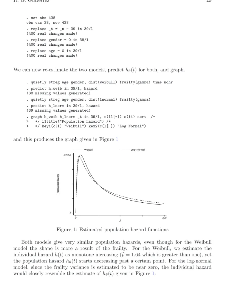
and this produces the graph given in Figure1.

Population hazard _t Weibull Log−Normal 0 399 0 .02056

Figure 1: Estimated population hazard functions

Both models give very similar population hazards, even though for the Weibull model the shape is more a result of the frailty. For the Weibull, we estimate the individual hazardh(t) as monotone increasing (p= 1.64 which is greater than one), yet the population hazardhθ(t) starts decreasing past a certain point. For the log-normal

model, since the frailty variance is estimated to be near zero, the individual hazard would closely resemble the estimate ofhθ(t) given in Figure 1.

(10)

2.4 Obtaining conditional predictions

The previous section serves to point out that predict used after a univariate frailty model will give population (unconditional) predictions. That is, the predictions are adjusted for the estimated frailty varianceθ and for the assumed frailty distribution. Should we want predictions that are instead conditional on arbitraryα, we would have to start from the hazard function given in (2) and work our way through to how α

enters into the prediction, given the functional form of the individual hazard, parameter estimates, and covariate values.

Of particular interest is the case whereα= 1, the mean frailty. When α= 1, pop-ulation or frailty-adjusted quantities such ashθ(t) reduce to their respective individual

quantities such ash(t). Predictions that condition onα= 1 are obtained via the option alpha1topredict.

For example, in order to compare the individual hazards for the Weibull/gamma ver-sus the Log-normal/gamma models, we repeat the previous example, this time utilizing thealpha1option:

. quietly streg age gender, dist(weibull) frailty(gamma) time nohr . predict ih_weib in 39/l, hazard alpha1

. quietly streg age gender, dist(lnormal) frailty(gamma) . predict ih_lnorm in 39/l, hazard alpha1

. graph ih_weib ih_lnorm _t in 39/239, c(ll[-]) s(ii) sort /* > */ l1title("Individual hazard") /*

> */ key1(c(l) "Weibull") key2(c(l[-]) "Log-Normal")

The above generates the graph shown in Figure2, and demonstrates the frailty eﬀect in the Weibull model.

Individual hazard _t Weibull Log−Normal 0 200 0 .140508

(11)

This technique may be used not only to obtain the predicted individual hazard, but to obtain any prediction conditional onα= 1. In general, sinceαis a scalar one may use the relationship in (2) to take a prediction that is conditional onα= 1 and transform it into a prediction conditional on anyα. For example, from (2) we getS(t|α) ={S(t)}α_,

and so if we wanted to predict the survival function conditional on α = 0.5, say, we would simply type

. predict S, surv alpha1 . replace S = S^0.5

Note: In general,predict, survcalculatesS(t)/S(t0), and so if you are usingpredict, survto obtainS(t) over a plotting grid of values of t, be sure to set t0equal to zero over that grid.

2.5 A note on hazard ratios

When we analyzed the kidney data in Section2.2, we ﬁt a Weibull/gamma model in the accelerated failure time metric (AFT). We chose this parameterization to ease the comparison with the log-normal model which is parameterized as AFT. However, we could just have easily estimated the Weibull model in the proportional hazards (PH) metric, since both parameterizations are available instreg.

. use kidney, clear . stset time1 fail1

(output omitted)

. streg age gender, dist(weibull) frailty(gamma) nolog failure _d: fail1

Weibull regression -- log relative-hazard form Gamma frailty

Time at risk = 3630

LR chi2(2) = 4.78 Log likelihood = -48.410833 Prob > chi2 = 0.0917 _t Haz. Ratio Std. Err. z P>|z| [95% Conf. Interval] age 1.018152 .0251684 0.73 0.467 .9699991 1.068696 gender .1109124 .1306617 -1.87 0.062 .0110208 1.116217 /ln_p .4965477 .31294 1.59 0.113 -.1168033 1.109899 /ln_the .3610336 .7067754 0.51 0.609 -1.024221 1.746288 p 1.643039 .5141726 .8897602 3.034051 1/p .6086282 .1904641 .3295923 1.123898 theta 1.434812 1.01409 .3590761 5.733281 Likelihood ratio test of theta=0: chibar2(01) = 4.20 Prob>=chibar2 = 0.020

(12)

The results are the same as before, except for the regression coeﬃcients, which are now parameterized in thePHmetric and displayed (by default) as hazard ratios.

In standard models, a hazard ratio is interpreted as a proportional shift in the hazard function due to a unit change in the associated covariate. When using a frailty model, however, reported “hazard ratios” carry this usual interpretation only if comparing two hazards conditional on a given α. For example, one would interpret the hazard ratio reported for the covariategender as “all other things equal (including the frailty α), the hazard function for females is 0.11 times the hazard for males”.

Unconditionally, however, the proportionality of hazards does not generally hold. When comparing two population hazards, for most distributions of the frailty the re-ported hazard ratios are only true hazard ratios at timet= 0. The exception to this rule is when the frailties follow a distribution from the positive stable family, in which case the hazard ratios remain constant over time; seeHougaard(1986b).

However, for those distributions of frailty currently in Stata, namely the gamma and inverse Gaussian, with the passage of time the eﬀect of the covariates on the population hazard will diminish in favor of the frailty eﬀect. In other words, with the passage of time, gender (for instance) becomes less of a factor and frailty becomes more of a factor in determining the chance of remaining infection free.

It is on this point where we can see a subtle, yet important, diﬀerence between the gamma and inverse Gaussian distributions. For gamma frailties, the relationship between individual and population hazards is

hθ(t) =h(t)[1−θln{S(t)}]−1

If we have an individual hazardh∗(t) =ch(t) for some constantc, thenS∗(t) ={S(t)}c and the ratio of the population hazards

h∗_θ(t)

hθ(t)

=h

∗₍_t_)[1₋_θ_ln_{_S∗₍_t₎_}_]−1

h(t)[1−θln{S(t)}]−1 equalscat t= 0 but will tend towards 1 as tgoes to inﬁnity.

For inverse Gaussian frailties, the relationship between the individual and population hazards is remarkably similar to that for gamma frailties

hθ(t) =h(t)[1−2θln{S(t)}]−1/2

However, in this case an individual hazard ratio ofc translates to a population hazard ratio equal tocatt= 0 tending towards√c astgoes to infinity. In other words, when the frailty is distributed as inverse Gaussian the effect of the covariates diminishes with time, but never completely vanishes as it does when frailties follow a gamma distribution. If estimating in theAFTmetric, however, the interpretation of regression coefficients remains the same, conditionally and unconditionally. Recall that in a standard (non-frailty) regression theAFTparameterization assumes that

(13)

for some baseline survival function S0(t) = S(t|x = 0), vector of covariates x, and regression coefficientsβ. That is, under this metric the effect of the covariates is to either accelerate or decelerate the effect of time on the probability of survival. Examination of (3) shows that this relationship still holds in a frailty model. That is,

Sθ(t) =Sθ0{exp(xβ)t}

withS0

θ(t) =Sθ(t|x=0).

3 Shared frailty models

A natural extension of the univariate frailty model would be a multivariate survival model where individuals are allowed to share the same frailty value. Sharing a frailty value also generates dependence between those individuals who share frailties, whereas conditional on the frailty those individuals are independent.

For data consisting of n groups with the ith group comprised of ni individuals

(i= 1, . . . , n), (2) generalizes to

hij(t|αi) =αihij(t)

forj = 1, . . . , ni withhij(t) =h(t|xij). That is, for any member of theith group, the

standard hazard function is now multiplied by the shared frailtyαi. For example, in

the case of WeibullPHregression, the conditional hazard for an individual is given by

hij(t|αi) =αihij(t) =αiexp(xijβ)ptp−1

and the conditional survival function is

Sij(t|αi) ={Sij(t)}αi = exp{−αiexp(xijβ)tp}

3.1 Derivation of the likelihood

The likelihood of the observed data is obtained by calculating the group-level conditional likelihoods and integrating out the frailty. Suppose we have data for i = 1, . . . , n

groups with j = 1, . . . , ni observations per group consisting of the trivariate response

(t0ij, tij, dij), which indicate the start time, end time, and failure/censoring for thejth

individual from theith group.

Givenαi, the contribution to the likelihood of theijth individual is thus Lij(αi) = Sij(tij|αi) Sij(t0ij|αi){ hij(tij|αi)}dij = Sij(tij) Sij(t0ij) α_i {αihij(tij)}dij

(14)

and if we deﬁneDi= n_i

j=1dij, the likelihood of theith group is Li(αi) =αDi i ni j=1 Sij(tij) Sij(t0ij) αi {hij(tij)}dij

Unconditionally, we can obtain the likelihood of theith group by integrating outαi, Li=

_∞

0

Li(αi)g(αi)dαi

where g() is the probability density function of the frailty, given by (4) in the case of gamma, and by (5) for the inverse Gaussian. When the frailties follow a gamma distribution,Li can be expressed compactly as

Li=  ni j=1 {hij(tij)}dij  Γ(1/θ+Di) Γ(1/θ) θ Di   1−θ ni j=1 ln Sij(tij) Sij(t0ij)    −1/θ−Di

When the frailties follow an inverse Gaussian distribution, the expression forLiis quite

complex, and involves integer half orders of the modiﬁed Bessel function of the third kind (commonly known as the BesselK function).

Given the unconditional group likelihoods, we can estimate the regression parameters and frailty varianceθby maximizing the overall log-likelihood lnL=n_i₌₁lnLi.

3.2 Kidney data revisited

Let’s once again consider the kidney data from Section2.2. This time, however, we’ll consider both recurrence times given for each patient. The data are in wide form, and so before westsetour dataset, we need toreshapeit into long form.

. use kidney, clear . gen patient = _n

. reshape long time fail, i(patient)

(output omitted)

. list patient time fail age gender in 1/10

patient time fail age gender 1. 1 16 1 28 0 2. 1 8 1 28 0 3. 2 13 0 48 1 4. 2 23 1 48 1 5. 3 22 1 32 0 6. 3 28 1 32 0 7. 4 318 1 31.5 1 8. 4 447 1 31.5 1 9. 5 30 1 10 0 10. 5 12 1 10 0 . stset time fail

(15)

Since it is reasonable to expect some correlation between the two recurrence times for a given patient, we can model this as a shared frailty model where the sharing takes place on the patient level. This is easily done by adding the option shared(patient) to our previous calls of streg, frailty().

First, we ﬁt a Weibull/gamma shared frailty model,

. streg age gender, dist(weibull) frailty(gamma) shared(patient) time nohr nolog failure _d: fail

analysis time _t: time

Weibull regression -- accelerated failure-time form Gamma shared frailty

Time at risk = 7424

LR chi2(2) = 14.81 Log likelihood = -98.006931 Prob > chi2 = 0.0006 _t Coef. Std. Err. z P>|z| [95% Conf. Interval] age -.0067052 .0102377 -0.65 0.512 -.0267707 .0133602 gender 1.506616 .3659291 4.12 0.000 .7894085 2.223824 _cons 3.557985 .5224117 6.81 0.000 2.534077 4.581894 /ln_p .2410369 .1336503 1.80 0.071 -.0209129 .5029866 /ln_the -.4546298 .4747326 -0.96 0.338 -1.385089 .475829 p 1.272568 .1700791 .9793043 1.653653 1/p .7858127 .1050241 .6047219 1.021133 theta .6346829 .3013047 .2503016 1.609348 Likelihood ratio test of theta=0: chibar2(01) = 10.87 Prob>=chibar2 = 0.000

and, as before, see a significant frailty effect when we assume that the marginal hazard is Weibull. Sahu et al.(1997) fit a Bayesian formulation of the above model estimated using Gibbs sampling, and obtained similar estimates to the maximum-likelihood esti-mates displayed above, with theirθ= 0.585 resembling our θ= 0.635.

Assuming a log-normal marginal hazard, however,

. streg age gender, dist(lnormal) frailty(gamma) shared(patient) nolog failure _d: fail

analysis time _t: time

Log-normal regression -- accelerated failure-time form Gamma shared frailty

Time at risk = 7424

LR chi2(2) = 16.65 Log likelihood = -97.594575 Prob > chi2 = 0.0002

(16)

_t Coef. Std. Err. z P>|z| [95% Conf. Interval] age -.0067002 .0098278 -0.68 0.495 -.0259623 .0125619 gender 1.422234 .3343544 4.25 0.000 .7669111 2.077556 _cons 3.331102 .4911662 6.78 0.000 2.368434 4.29377 /ln_sig .0670784 .1187767 0.56 0.572 -.1657197 .2998764 /ln_the -1.823592 .995803 -1.83 0.067 -3.77533 .1281455 sigma 1.069379 .1270173 .8472837 1.349692 theta .1614447 .1607671 .0229295 1.136718 Likelihood ratio test of theta=0: chibar2(01) = 1.57 Prob>=chibar2 = 0.105

we find the frailty to be insignificant at the 10% level. As in Section2.2, it is of interest to determine which model better fits the data, the Weibull model with significant frailty effect, or the log-normal model with insignificant frailty.

In order to answer that question, we follow the lead ofSahu et al.(1997), who also fit via Gibbs sampling a piecewise exponential model (piecewise constant hazard) with shared frailty. This requires that we firststsplitour records so that we can generate the appropriate indicator variables that specify the pieces. However, before we do that we need to re-stsetour dataset and assign each record a unique identifier variable.

. gen obs = _n

. stset time fail, id(obs)

(output omitted)

. stsplit my_t, at(1(1)562) /* 562 is the max(_t) */ (7348 observations (episodes) created)

Note that we still plan on sharing frailties at the patient level, and the variable obs used above merely uniquely identiﬁes the individual observations (distinct recurrences of infection) for purposes of splitting the records. Once we split the records, we generate the indicator variables, which comprise a grid of ten intervals spanning [ 0,60), [ 60,120), . . . , [ 480,540), [ 540,∞).

. forvalues k = 1/9 {

2. gen in_‘k’ = ((‘k’-1)*60 <= my_t) & (my_t < ‘k’*60) 3. }

and the indicators are constructed so that the baseline interval (that for which all the indicators equal zero) is the interval [ 540,∞).

We are now ready to ﬁt the piecewise exponential/gamma shared frailty model.

. streg age gender in_*, dist(exp) frailty(gamma) shared(patient) nolog nohr time failure _d: fail

analysis time _t: time id: obs

(17)

Exponential regression -- accelerated failure-time form Gamma shared frailty

Time at risk = 7424

LR chi2(11) = 20.90 Log likelihood = -95.241838 Prob > chi2 = 0.0344 _t Coef. Std. Err. z P>|z| [95% Conf. Interval] age -.0060301 .0119445 -0.50 0.614 -.0294409 .0173807 gender 1.416426 .4525747 3.13 0.002 .5293963 2.303456 in_1 2.566041 1.350038 1.90 0.057 -.0799854 5.212067 in_2 3.229574 1.339194 2.41 0.016 .6048016 5.854347 in_3 2.366064 1.29691 1.82 0.068 -.1758328 4.907961 in_4 2.1349 1.305189 1.64 0.102 -.4232243 4.693024 in_5 2.44805 1.373428 1.78 0.075 -.2438189 5.139919 in_6 2.788362 1.52622 1.83 0.068 -.2029743 5.779697 in_7 2.659777 1.518699 1.75 0.080 -.3168189 5.636373 in_8 2.319784 1.501516 1.54 0.122 -.6231325 5.262701 in_9 1.233349 1.296951 0.95 0.342 -1.308628 3.775326 _cons 1.057467 1.488013 0.71 0.477 -1.858986 3.973919 /ln_the -.8007126 .5527555 -1.45 0.147 -1.884094 .2826683 theta .4490089 .2481921 .1519667 1.326665 Likelihood ratio test of theta=0: chibar2(01) = 6.62 Prob>=chibar2 = 0.005

The estimated frailty variance using maximum likelihood, θ= 0.449, again compares favorably with the Bayesian estimate of the related model of Sahu et al. (1997), for whomθ= 0.499. After assuming a more ﬂexible individual hazard, the results seem to favor the Weibull model over the log-normal, and we now have stronger evidence of the existence of latent patient frailty.

3.3 Obtaining conditional predictions

When one speciﬁes the option shared()with streg, frailty(), the default predic-tions obtained from predict are conditional on αi = 1 for all i = 1, . . . , n. This is

diﬀerent from whenshared()is not speciﬁed (see Section2.3), in which case predict will give unconditional predictions that are averaged over the distribution ofα.

The main reason for this change in behavior inpredictwhen going from a univariate frailty model to a shared frailty model has to do with the interpretation of “population” functions likehθ(t) and Sθ(t). In a non-shared frailty model the interpretation is

rela-tively straightforward — the functionSθ(t) is the new generalized survival function with

all the usual interpretations and from which all the likelihood calculations are derived. In a shared frailty model, however, the functionSθ(t) from (3) is not always a true

survival function in the strictest sense. For example, consider a hypothetical popula-tion of groups where the relative size of each group is correlated with the frailty for

(18)

that group. In this case the use ofSθ(t) to estimate population dynamics such as the

proportion of the population that survives past a given timetwould lead to misleading results. One can get around this problem by interpretingSθ(t) as giving the probability

of survival, say, of a randomly chosen individual from a randomly chosen group, or by assuming (and carefully checking the assumption) that group size is orthogonal to frailty. In any case, there are diﬃculties with having a statement such as

. predict S, surv

which implies that one is getting the population “survival” function, when in fact this might not be the case. Of course, we may still be interested in obtaining an estimate ofSθ(t) if we are willing to make the appropriate assumptions as to its interpretation,

and this is easily accomplished as shown in Section3.4.

For now, however, we can usepredict to obtain the estimated individual hazard functions (givenαi= 1) for the three shared frailty models we have already ﬁt.

. reshape long time fail, i(patient)

(output omitted)

. gen obs = _n

. stset time fail, id(obs)

(output omitted)

. stsplit my_t, at(1(1)562) /* _N == 7424, now */ (7348 observations (episodes) created)

. set obs 7824 /* add 400 observations for graphing */ obs was 7424, now 7824

. replace _t = _n - 7424 in 7425/l /* generate graphing grid */ (400 real changes made)

. replace my_t = _t in 7425/l /* indicators for exp graph */ (400 real changes made)

. replace gender = 0 in 7425/l /* baseline for graphs */ (400 real changes made)

. replace age = 0 in 7425/l (400 real changes made) . forvalues k = 1/9 {

2. gen in_‘k’ = ((‘k’-1)*60 <= my_t) & (my_t < ‘k’*60) 3. }

. quietly streg age gender in_*, dist(exp) fr(gamma) sh(patient) nohr time . predict h_exp in 7425/l, hazard

. quietly streg age gender, dist(weibull) fr(gamma) sh(patient) nohr time . predict h_weib in 7425/l, hazard

. quietly streg age gender, dist(lnormal) fr(gamma) sh(patient) . predict h_lnorm in 7425/l, hazard

(19)

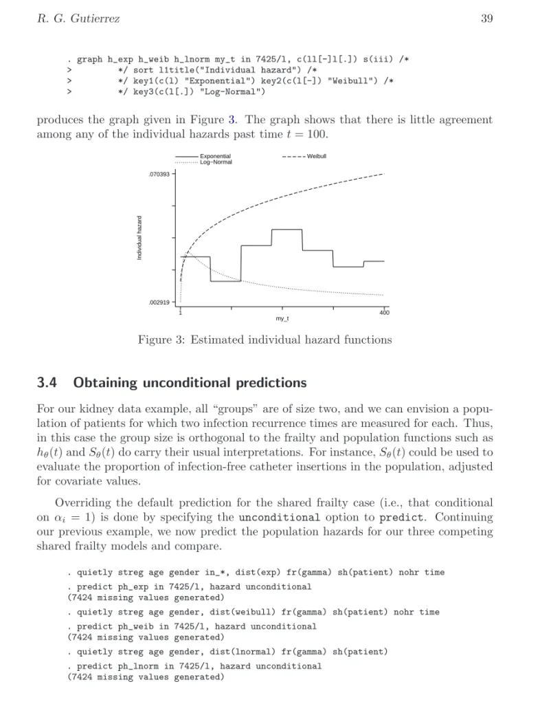
. graph h_exp h_weib h_lnorm my_t in 7425/l, c(ll[-]l[.]) s(iii) /* > */ sort l1title("Individual hazard") /*

> */ key1(c(l) "Exponential") key2(c(l[-]) "Weibull") /* > */ key3(c(l[.]) "Log-Normal")

produces the graph given in Figure3. The graph shows that there is little agreement among any of the individual hazards past timet= 100.

Individual hazard my_t Exponential Weibull Log−Normal 1 400 .002919 .070393

Figure 3: Estimated individual hazard functions

3.4 Obtaining unconditional predictions

For our kidney data example, all “groups” are of size two, and we can envision a popu-lation of patients for which two infection recurrence times are measured for each. Thus, in this case the group size is orthogonal to the frailty and population functions such as

hθ(t) andSθ(t) do carry their usual interpretations. For instance,Sθ(t) could be used to

evaluate the proportion of infection-free catheter insertions in the population, adjusted for covariate values.

Overriding the default prediction for the shared frailty case (i.e., that conditional onαi = 1) is done by specifying the unconditional option topredict. Continuing

our previous example, we now predict the population hazards for our three competing shared frailty models and compare.

. quietly streg age gender in_*, dist(exp) fr(gamma) sh(patient) nohr time . predict ph_exp in 7425/l, hazard unconditional

. quietly streg age gender, dist(weibull) fr(gamma) sh(patient) nohr time . predict ph_weib in 7425/l, hazard unconditional

. quietly streg age gender, dist(lnormal) fr(gamma) sh(patient) . predict ph_lnorm in 7425/l, hazard unconditional

(20)

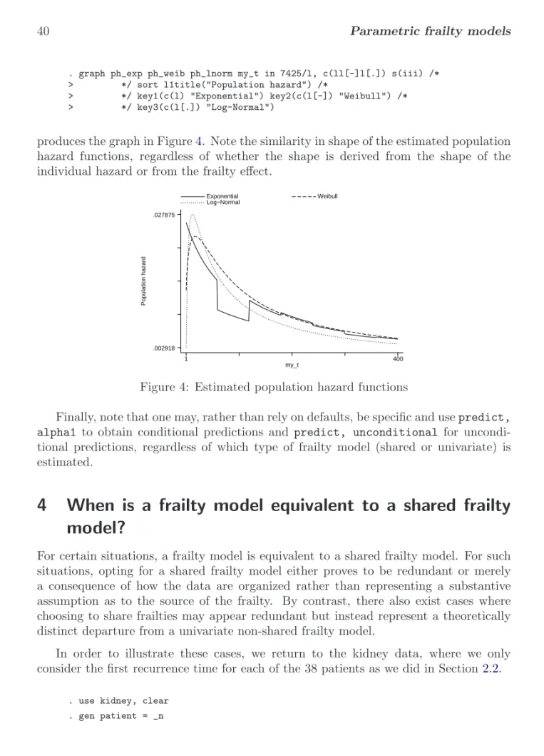
. graph ph_exp ph_weib ph_lnorm my_t in 7425/l, c(ll[-]l[.]) s(iii) /* > */ sort l1title("Population hazard") /*

> */ key1(c(l) "Exponential") key2(c(l[-]) "Weibull") /* > */ key3(c(l[.]) "Log-Normal")

produces the graph in Figure4. Note the similarity in shape of the estimated population hazard functions, regardless of whether the shape is derived from the shape of the individual hazard or from the frailty eﬀect.

Population hazard my_t Exponential Weibull Log−Normal 1 400 .002918 .027875

Figure 4: Estimated population hazard functions

Finally, note that one may, rather than rely on defaults, be speciﬁc and usepredict, alpha1 to obtain conditional predictions and predict, unconditional for uncondi-tional predictions, regardless of which type of frailty model (shared or univariate) is estimated.

4 When is a frailty model equivalent to a shared frailty

model?

For certain situations, a frailty model is equivalent to a shared frailty model. For such situations, opting for a shared frailty model either proves to be redundant or merely a consequence of how the data are organized rather than representing a substantive assumption as to the source of the frailty. By contrast, there also exist cases where choosing to share frailties may appear redundant but instead represent a theoretically distinct departure from a univariate non-shared frailty model.

In order to illustrate these cases, we return to the kidney data, where we only consider the ﬁrst recurrence time for each of the 38 patients as we did in Section2.2.

(21)

. list patient time1 fail1 age gender in 1/10

patient time1 fail1 age gender 1. 1 16 1 28 0 2. 2 13 0 48 1 3. 3 22 1 32 0 4. 4 318 1 31.5 1 5. 5 30 1 10 0 6. 6 24 1 16.5 1 7. 7 9 1 51 0 8. 8 30 1 55.5 1 9. 9 53 1 69 1 10. 10 154 1 51.5 0

4.1 Singleton groups of complete observations

We deﬁne acomplete observation to be a single record representing a time span that begins at timet = 0 and ends either in failure or right-censoring, in other words, the most simple form of survival data. For the kidney data given above, the entry time

t= 0 is assumed for each patient since we do not specify otherwise when westsetthe data.

. stset time1 fail1, id(patient)

(output omitted)

. list patient _t0 _t age gender in 1/5

patient _t0 _t age gender 1. 1 0 16 28 0 2. 2 0 13 48 1 3. 3 0 22 32 0 4. 4 0 318 31.5 1 5. 5 0 30 10 0

Since we have only one observation per patient, specifying id(patient) when we stset our dataset is for most purposes not necessary, but we do so anyway because we plan onstsplitting the dataset later.

In this case, when ﬁtting a frailty model whether we choose to share the frailties on the patient level does not matter, and we would get identical results for either model. In order to save space, we demonstrate this fact by only displaying the log likelihoods for each model, but in fact all the parameter estimates, standard errors, etc. would also be identical.

. quietly streg age gender, dist(weibull) frailty(invgauss) . display e(ll)

-49.253638

. quietly streg age gender, dist(weibull) frailty(invgauss) shared(patient) . display e(ll)

(22)

The above seems obvious given that we are sharing frailties on groups each consisting of one observation, but as we illustrate below, this is only true because we have singleton groupsandeach singleton observation is complete.

4.2 Singleton groups with left-truncation

Left-truncated observations are those for which subjects are not observed beginning at

t= 0 but instead initially come under observation at some timet0 >0. For example, suppose we now assume that our 38 patients came under observation at timet= 1; i.e., by the time we initially observe each patient, he has already been infection free up to timet= 1. Otherwise we would not have observed him. We represent this assumption by specifying an entry time equal to 1 when westsetour dataset,

. stset time1 fail1, id(patient) enter(time 1)

(output omitted)

. list patient _t0 _t age gender in 1/5

patient _t0 _t age gender 1. 1 1 16 28 0 2. 2 1 13 48 1 3. 3 1 22 32 0 4. 4 1 318 31.5 1 5. 5 1 30 10 0

and observe that the only diﬀerence is that now t0==1for all observations.

In cases where some or all observations are not complete but are instead left-truncated, sharing frailties at the patient level will result in a diﬀerent estimation, even though the sharing still takes place across singleton groups.

-49.075185

-49.063301

In this case, since the observations are not complete, whether we share frailties at the patient level is relevant to what we assume about the model. If we do not share frailties, we assume that each patient has a spell-speciﬁc frailty for the unobserved period (0,1] and a diﬀerent frailty for the period afterwords. For example, we can think of the frailty as representing a latent time-dependent covariate with unique values over each period. However, when we do share frailties at the patient level, for each patient the frailties for the two periods (unobserved and observed) are assumed equal. In this case, the frailty may represent a latent covariate that is unique to each patient, yet constant over time. That the period (0,1] is unobserved doesn’t matter since although we do not observe the patient over this period, we still condition on the patient’s survival to the end of that period when evaluating the likelihood.

(23)

4.3 Uninformative episode splitting

Stata’s st family of commands are well-suited for dealing with multiple records per individual, with each record representing the time span (t0, t]. Using multiple records is necessary to deal with time-varying covariates, left truncation, and gaps in which subjects are left unobserved. In cases where multiple records are utilized for any or all of these purposes, the splitting of episodes for a given individual is said to beinformative. Informative episode splitting, for reasons described previously assuming that frailties are shared over these episodes, yields diﬀerent parameter estimates than those obtained by not sharing frailties and by instead assuming that the frailties are episode-speciﬁc.

However, sometimes multiple records exist for individuals as a result of how the data were collected or organized, and the splitting of records does not reﬂect time-varying covariates, left truncation, or observation gaps. The splitting of records in this case is uninformative, and the records could be collapsed into single complete observations without any loss or change of information. In these situations, sharing frailties on the groups formed by having what are really complete observations that have been split uninformatively will produce the same results as if the frailties had not been assumed shared.

To illustrate, let’sstsplit the complete observations in our kidney data to form a dataset containing multiple records for each patient.

. stset time1 fail1, id(patient)

(output omitted)

. stsplit my_t, at(5(5)562)

(702 observations (episodes) created)

. list patient _t0 _t age gender if patient <= 3

patient _t0 _t age gender 1. 1 0 5 28 0 2. 1 5 10 28 0 3. 1 10 15 28 0 4. 1 15 16 28 0 5. 2 0 5 48 1 6. 2 5 10 48 1 7. 2 10 13 48 1 8. 3 0 5 32 0 9. 3 5 10 32 0 10. 3 10 15 32 0 11. 3 15 20 32 0 12. 3 20 22 32 0

Since the splitting was done arbitrarily beginning with a dataset comprised of complete observations, the splitting of records is uninformative with no loss, gain, or change in the information contained in the complete observations. As a result, a model with frailties shared over the multiple records for each patient is equivalent to one with frailties shared on the singleton groups of complete observations, and this in turn is equivalent to a model where the frailties are not shared.

(24)

-49.253638

5 References

Clayton, D. 1978. A model for association in bivariate life tables and its applications in epidemiological studies of familial tendency in chronic disease incidence. Biometrika 65: 141–151.

Clayton, D. and J. Cuzick. 1985. Multivariate generalisations of the proportional hazards model (with discussion). Journal of the Royal Statistical Society, Series A148: 82– 117.

Hougaard, P. 1984. Life table methods for heterogeneous populations: Distributions describing the heterogeneity. Biometrika71: 75–83.

—. 1986a. A class of multivariate failure time distributions. Biometrika73: 671–8. —. 1986b. Survival models for heterogeneous populations derived from stable

distribu-tions. Biometrika73: 397–96.

—. 1995. Frailty models for survival data. Lifetime Data Analysis 1: 255–273.

Lancaster, T. 1979. Econometric methods for the duration of unemployment. Econo-metrica47: 939–56.

McGilchrist, C. A. and C. W. Aisbett. 1991. Regression with frailty in survival analysis. Biometrics 47: 461–466.

Sahu, S. K., D. K. Dey, H. Aslanidou, and D. Sinha. 1997. A Weibull regression model with gamma frailties for multivariate survival data. Lifetime Data Analysis 3: 123– 137.

Vaupel, J. W., K. Manton, and E. Stallard. 1979. The impact of heterogeneity in individual frailty on the dynamics of mortality. Demography 16: 439–54.

Whitmore, G. A. and M.-L. T. Lee. 1991. A multivariate survival distribution generated by an inverse Gaussian mixture of exponentials. Technometrics33: 39–50.

About the Author