Optimal power control strategy of a hybrid energy system considering
demand response strategy and customer interruption cost
O. Dzobo*
a, Y. Sun
aaDepartment of Electrical & Electronic Eng. Science, University of Johannesburg, Johannesburg, South Africa.
Abstract: The integration of distributed renewable energy sources into the conventional power system network have created opportunities for electricity customers to reduce their electricity cost. This paper investigates the optimal power scheduling of a hybrid energy system connected to the grid in the presence of demand response strategy and inconvenience cost. A new proposed method of calculating the inconvenience cost which is dependent on total home appliance load, customer interruption cost (CIC) and delay time operation of home appliances is proposed. The hybrid energy system consists of solar photovoltaic (PV) module and battery bank storage system. The home appliance scheduling is formulated as a non-convex mixed integer programming with a binary decision variable to switch ON/OFF the home appliances. The optimization objective is to minimize both the total daily electricity cost and inconvenience cost of a residential customer with different time shiftable, power shiftable home appliances and customer time preference constraints. The results show that it is important to schedule home appliances and include their inconvenience cost so that home appliances are not only shifted to the lower electricity tariff periods but can also start at their customer preferred operation times. The results also show that the hybrid energy system is able to cater for all the energy requirements of home appliances during the day, reducing power demand from grid by a significant percentage and thus relieve the power system network and afford electricity consumers significant monetary savings.
Keywords: Battery bank storage, customer interruption cost, demand response, electricity cost/bill, home appliance scheduling, solar PV module system.
1. INTRODUCTION
Demand side management (DSM) plays an important role in facilitating the integration of distributed renewable energy sources into the conventional power system network. It has been estimated that it could translate into as much as US$59 billion in societal benefits by 2019 [1]. DSM programs can be categorized as demand response (DR) programs and energy efficiency programs. In DR programs the electricity consumers are given incentives to shift their loads during periods of peak demands [2, 3]. This reduces the stress on the power system network and allows for more electricity to be provided to customers with less expensive base load generation [4, 5]. Traditionally, DR programs have been applied to large electricity consumers such as industrial or commercial buildings [3]. These mechanisms are still very rare in residential customers where the implementation costs were considered to be relatively high. However, recent advances in integration of hybrid energy systems and development of smart home appliances have led to a new dimension of research to optimize the power control strategies between the power utility and the residential customer [6]. *Address correspondence to this author at the Department of Electrical & Electronic Eng. Science, University of Johannesburg, Johannesburg, South Africa, Tel/Fax: +27-11-559-4010, +27-11-559-2344; E-mails: [email protected]
Residential customers perform different daily activities during the day. These daily activities are characterized by different home appliances that are scheduled to operate at preferred time intervals [7]. Some of the home appliances are continuously connected throughout the whole day, e.g., refrigerator. These type of home appliances consume electricity throughout the day and have mechanisms to adjust their electricity consumption levels. In some cases, the home appliances are scheduled to run sequentially in order to complete a task or an activity. Many research studies have been done to minimize the electricity cost of residential customers through optimally scheduling their home appliances [8, 9]. However, in some research studies the constraints considered ignore that home appliances may have to run sequentially without interruption resulting in home appliances being scheduled at inconvenience times which may be inappropriate for their operation. It is therefore important to reveal further the resultant home appliance schedule achieved from the minimization of load and electricity cost to ascertain whether the load or cost reduction is not achieved as a result of inappropriate scheduling of the home appliances. The cost of scheduling home appliances at inconvenience times is commonly considered as inconvenience cost [8]. In most research studies, the inconvenience costs due to postponement of home appliance schedules are estimates from the load not supplied [8].
However, the activity interruption cost incurred by the customer as a result of deferring some of their daily activities is not always equal to the energy not supplied or energy saved [10]. In most cases, the activity interruption cost incurred by electricity customers is far more than the energy not saved. Several research studies have been done to ascertain the cost of power supply interruption to different electricity customers daily activities [11, 12]. Generally, the cost due to power supply interruption of customer daily activities is represented as a customer damage function model [11, 13]. A customer damage function model is a linear representation of cost incurred by electricity customers whenever a power supply interruption occurs. This cost due to power supply interruption on residential customer daily activities is commonly referred to as customer interruption cost (CIC) [13]. The cost incurred by electricity customers is studied for different durations, seasons, time of day etc [13, 14]. In most cases, the customer damage function model is developed using customer interruption cost (CIC) estimates from customer surveys [11]. This is a good representation of the cost of power supply interruption to the daily activities of electricity customers since the cost estimates are taken from the electricity customers themselves. In this paper, a new hybrid energy system optimization model which uses the customer damage function model to represent the cost incurred by electricity customers due to postponement of their daily activities is proposed. The customer damage function model considered in this paper is taken from a customer survey performed in Cape Town, South Africa [15].
General home appliance scheduling models without storage and/or renewable energy sources are presented in [16, 17, 5]. On the other hand, the application of renewable energy sources, e.g., solar PV energy systems, and battery bank energy storage systems in residential customers is considered without home appliance scheduling problem in [18, 19, 20, 21]. The main disadvantage of decoupling home appliance scheduling models and renewable energy sources including energy storage systems is that the cost saving opportunities that may exists between their interdependency is ignored [9]. Thus, the decoupled optimization models may forge suboptimal electricity consumption behavior as well as higher electricity costs than they would otherwise in a optimally efficient interdependent energy systems [21]. A review of the modeling techniques, solving methods, reliability, emission, uncertainty, stability, demand response(DR), and multi-objective standpoint in the microgrid and Virtual Power Plants frameworks were presented [22, 23, 24]. The authors pointed the same concern about the exclusion of demand response strategies in optimization control of smart grids. The purpose of this paper is to formulate a practical optimization model for a residential customer in order to determine the optimal home appliance scheduling that simultaneously minimizes their daily electricity cost/bill and inconvenience cost. A case study of a hybrid energy system consisting of a solar PV module and battery bank storage system is presented.
The main contributions of the paper are:
(i) A new model that includes the customer damage function model to estimate the inconvenience cost due to postponement of residential customer home appliances time of operation.
(ii) The constraints for time-shiftable and power shiftable home appliances are included in the
analyses. The optimization model also includes constraints for home appliances to run sequentially without interruption and customer preference for home appliance to operate within particular time intervals at different energy consumption levels. (iii)The results show the electricity cost savings or
reduction in demand during peak hours with the actual schedule of the home appliances presented. The rest of the paper is organized as follows: Section 2 introduces the DR mathematical problem formulation; Section 3 presents the case study. Section 4 covers the numerical simulations using mixed binary integer linear programming on two scenarios and present obtained results. The conclusion is presented in Section 5.
2. PROPOSED MATHEMATICAL CALCULATION METHODOLOGY
In this section, the proposed calculation methodology for total daily electricity cost and the inconvenience cost is outlined.
2.1. Total daily electricity cost
EcTo calculate the total daily electricity cost
Ec , the homeappliance load at each given hour
h and the permissiblepower utility maximum hourly load
U h must be known. Let A denote the set of home appliances for a residential customer. For each home appliance aA, the hourly home appliance demands are fixed constants during their operation periods. The home appliance demand scheduling vector Lafor the
entire scheduling horizon (H) is given by Eqs. 1 and 2.
1, ,... ,...
2 h H
(1)
a a a a aL
L L
L
L
,
0
(2)
h h a a h a a AL
L
U
a
A L
whereLhaLhfixed a, + Lhflexible a, ,
,
i.e,
sum of fixed andflexible home appliance loads at any given hour h
.
U h is the permissible power utility maximum total hourly load and is limited by the power utility. This constraint is important to avoid simultaneous scheduling of home appliances at the same time. In this paper, the maximum total hourly load limit is set at Uh2400W.Flexible home appliances are operated in optional time intervals. The residential customer is willing to defer its use for a later time or can be readily adjusted according to electricity price signals, e.g., water boiler, vacuum cleaner etc. The total load due to flexible home appliances at each given hour Lhflexible a, ,is calculated using the calculation model
explained in detail in ref [9]. The calculation model uses a binary switching vector, S
a, to select the optional operating
time interval of flexible home appliances. By using the binary integer switching vector, S
a, the home appliance demand
scheduling vector Lhflexible a, , is calculated as in Eqn. 3:
, , ,
(3)
T C T
flexible a flexible a flexible a flexible
L
L
S
a
A
where LTflexible a, , is the
H
H
, circulant matrix of thefundamental home appliance load demand pattern given as ,
c L
2 2 1 3 , 1 1 n H a a a C a a a flexible a H H a a a
L
The binary integer switching vector S
a, is defined as:
1, ,...,2 ,. ..
, , h H Sflexible a sa sa sa sa where h ,
0;1 ,
1, 2,...,
;
24.
flexible as
h
H
H
It has onlyone non-zero element that is equal to one (1) to ensure that the home appliance is switched ON only once during each operation. The position of the non-zero element in the binary integer switching vector indicates the time slot, ( )h , at which
the home appliance is switched ON. For home aA, this
constraint is written as in Eqn. 4:
1 (4) , 1 H h Sflexible a h
The fixed home appliances are switched ON and operate in fixed predetermined time intervals, e.g. lights, hand iron etc. The user would not defer the use of these home appliances to participate in demand response program as they impact heavily on their benefit. For example, security lights cannot be switched OFF during the night period as this pose a great security risk to the residential customer. For fixed home appliances the scheduling controller (SC) should know the beginning of acceptable operation time, fixed a, , end of the
acceptable operation time, ,
fixed a
, and acceptable operation
time of the appliance, Z ,
fixed a– where 1
, , ;
Z fixed afixed afixed a . The SC should finish
operation of the home appliance a A
fixed , by deadline i.e. the operation should be scheduled between fixed a, and
,
fixed a
. Given the pre-set parameters L ,
fixed a, Zfixed a, , ,
fixed a
and ,
fixed a
, the total energy consumed, E ,
fixed a, during the scheduling horizon is given by Eqn. 5
, , , , 1 , , , 0, , , ,
(5)
hLfixed a afixedA Zfixed a fixed a fixed a h Zfixed a
Lfixed a
h
Lfixed a h fixed aandh fixed a
Eq. 5 ensures that the home appliance operates during its acceptable operation time only and the total home appliance energy consumption during the scheduling horizon is equal to the total energy requirement for the home appliance operation. The aggregated residential customer home appliances load data used in this paper is presented in Table 1. The scheduling horizon ( )h for the home appliances is assumed to be 1 hour.
The total hourly energy consumption of the vacuum cleaner, television (TV) and cooker are assumed to be the average hourly energy consumption in this paper.
After getting the home appliance load as outlined above, the total daily electricity cost,
Ec , is then calculated. In most1 See:
http://www.eskom.co.za/CustomerCare/TariffsAndCharges- /WhatsNew/Documents scheduleStdPrices2015_16_27
research studies of DR programs in the literature, different techniques and algorithms to minimize total daily electricity cost of consumers are proposed [16, 25]. Commonly, time-dependent electricity pricing scheme, e.g., time-of-use (TOU) electricity pricing scheme, is applied in many power utilities. In this type of tariff scheme, the electricity price is varied throughout the day according to time of day and/or season in order to encourage electricity consumers to change their electricity consumption behavior. By having more electricity consumers that are willing to curtail their home appliance loads during periods of higher electricity tariffs and/or shift the flexible home appliance loads to periods of lowest electricity tariffs, both the power utility and the electricity consumers are able to save revenue [26, 27, 28]. Fixed electricity pricing scheme has also been applied in some research studies [25]. The main disadvantage of this tariff scheme is that there is a disconnection between the electricity price rates paid by electricity consumers and the short-term power generation costs. This may lead to inefficient electricity consumption behavior by electricity consumers as they do not adjust their home appliance loads to suit the supply side conditions. Therefore, fixed electricity pricing schemes may result in suboptimal power control strategies by not taking advantage of the home appliance load shifting capabilities. In this paper, actual TOU electricity pricing scheme used in South Africa is adopted. The TOU electricity pricing scheme uses average hourly electricity charges for residential customers.
Let the electricity price vector denote the time of use
electricity price rate for a day i.e.
1 2, ,..., h,..., H , h 0
.The residential customer
utilizes the electricity pricing data to schedule home appliances in order to minimize the total daily electricity cost. The total home appliance load at each time slot, h, is given by a A aLh.Therefore, the total electricity cost at each time slot, h, is calculated as in Eqn. 6.
(6) h h h h Ec La La a A a A
where LhaLhfixed a, + Lhflexible a, ,, i.e, sum of fixed and
flexible home appliance loads at any given hour h. The TOU electricity tariffs used in this paper are obtained from Eskom's 2015/16 Tariff book1 and are shown in Table 2 below. The
non-negative constant electricity prices are given in South African Rands (RSA) per kWh. 1US$ 15 RSA.
2.2. Inconvenience cost
Household activities tend to follow a daily pattern. When residential customers defer the use of their home appliances they incur an inconvenience cost. Several hypothetical inconvenience costs have been included in optimization of home appliance scheduling. However, home appliances are quite different and thus the inconvenience cost incurred by the residential customer is also diverse. This implies that residential customers need to be asked to estimate the inconvenience cost to their daily activities as it vary on daily and hourly basis. This creates an opening for a new approach
to estimate the temporal variations of inconvenience costs of residential customers.
To be able to quantify the temporal variations of inconvenience cost, customer valuations of how these effects
of disruption affect the inconvenience experienced by residential customers is needed. Commonly, in most residential customer surveys, these valuations are often included and made on an inconvenience scale [29]. The
Table 1: Aggregate electricity customer appliance loads
Appliance Type Ea (Wh)
α
a(h)β
a (h)) Za (h Inflexible Lights (8) Non-Shiftable 36 7 9 3 12 14 3 200 18 22 5 150 23 6 9Hand iron Non-Shiftable 250 17 17 1
Flexible Cooker Shiftable 750 7 9 1 12 14 1 20 22 1 Television Shiftable 70 7 10 2 12 15 2 20 23 2
Vacuum Cleaner Shiftable 400 10 12 2
20 22 2
Inflexible without inconvenience
Refrigerator (3) Power shiftable Hourly consumption = 350Wh - 540Wh Daily energy requirement = 10kWh
1 24 24
Air Conditioner Non-shiftable (Customer preference) Hourly consumption = 1kWh 12 16 5
20 22 3
Water boiler -
Power shiftable (Customer preferences) Hourly energy consumption = 0 - 1kWh
Total energy requirement = 1kWh 3 8 -
Total energy requirement = 1kWh 9 16 -
Total energy requirement = 1kWh 17 20 -
EV Power shiftable (Customer preference) Hourly consumption = 0.1 - 1.5kWh 21 9 -
Daily energy requirement = 5kWh
Table 2: TOU electricity prices for residential electricity customers in South Africa
Time (h) 1 2 3 4 5 6 7 8 9 10 11 12
TOU prices (RSA/kW h) 40:88 40:88 40:88 40:88 40:14 64:13 92:93 92:93 92:93 64:13 64:13 64:13
Time (h) 13 14 15 16 17 18 19 20 21 22 23 24
TOU prices (RSA/kW h) 64:13 64:13 64:13 64:13 64:13 92:93 92:93 64:13 64:13 40:88 40:88 40:88
values of the inconvenience scale are not used in absolute terms but rather to identify how residential customers rank the effect of power supply interruption on their daily activities.
Such studies have been done by [14], where different household activity levels were calculated at different times of day. Fig 1 shows the results from such a research study.
Place Fig 1 here
To capture the CIC incurred by residential customers during power supply interruption on their daily activities, contingent valuation methods are commonly used. In contingent valuations, residential customers are asked how much they are willing to pay (WTP) to avoid power supply interruption on their daily activities or how much they are willing to accept (WTA) a power supply interruption on their daily activities. Fig 2 shows the CIC of residential customers in Cape Town, South Africa used in this paper [15]. The CDF model is defined by line curve ABCD. Generally, the CIC increases as the duration of power supply interruption to residential customer daily activities increases. However, it can be clearly seen that as the duration of power supply interruption increases beyond 1.25 hours the rate of increase of CIC decreases. The least rate of increase of CIC is when the duration of power supply interruption to residential customer daily activities is between 1.25hrs and 4hrs.
Place Fig 2 here
The CIC values are constrained between the studied duration of power supply interruption. The CIC values for any given duration of power supply interruption to residential customer daily activities are defined by Eqs. 7 and 8.
2.83 9.7925 1.25 0.32( 1.25) 13.33 1.25 4 (7) 2.72 3.38( 4) 13.65 4 11 7 h if h CIC h if h h h if h
0
h
11
(8)
In the proposed model, the inconvenience cost is dependent on the home appliance load, CIC and operation delay time of the home appliance. The inconvenience cost for each home appliance, ICh
a,, at any given hour, h, is formulated as a quadratic function as in Eq. 9.
0 , , 0 2 0
(
, ,)
(9)
a h a h h h a a a h a hIC
L
CIC
wherea h, ,and a h0, ,are the baseline and optimal switching times of home appliance a at time h,. The quadratic function is preferred in this paper in order to increase the inconvenience cost exponentially as home appliance is shifted from its baseline switching time. The total inconvenience cost (IC) for all the home appliances is given as in Eqn. 10 subject to Eqn. 11 and 12. 0 , , 0 2 0 , , 1
(
)
(10)
a h a h H h a a h a h a A hIC
L
CIC
a
A
subject to 0 , ,11
(11)
a h a h
00
11
(12)
where 0, is the weighting factor based on how much emphasis is given to inconvenience cost by the residential
customer over the financial cost. Constraint 11 ensures that each home appliance is not shifted by more than 11 hours from its baseline switching time. This is because the maximum duration of power supply interruption for the CDF used in this research study is 11 hours. Constraint 12 ensures that the weighting factor lies between 0 and 1.
3. CASE STUDY: HYBRID ENERGY SYSTEM
The integration of renewable energy sources and demand response models in the conventional power system network is a new global research dimension for smart grids. In most research studies the most common renewable energy source considered for residential customers is the roof-top solar PV energy system [18]. However, the main disadvantage of solar PV energy systems has been identified as the dependency of its power output on intermittent solar radiation incident on the solar PV module. Several research authors have modelled the power output values of the solar PV energy system as stochastic values [19, 20]. This is intended to take into consideration the probability of occurrence of cloud cover on the solar PV module. However, in most cases, one probability distribution profile is used to represent the power output profile of the solar PV module and thus neglecting the time dependency of solar radiation levels during specific time periods of the day. In this paper, average solar PV module power output values for a case study location in South Africa are used in the analysis.
Small-scale renewable generation grids for residential customers have presented a lot of challenges to power system operators. The two main challenges are that of reverse power flows and metering solutions. In South Africa, the use of smart meters with bi-directional flow of power is still very limited. Therefore, in this paper, a solar PV module with battery bank storage system, without in-feed to the grid is considered. Figure 3 shows the power flows for the hybrid energy system model considered in this paper. The maintenance and operation costs of the solar PV module and battery bank are not considered in the analysis. The hybrid energy system is designed for maximum use of solar PV module. Thus, at each time slot h the total home appliance electricity demand is
supplied by the solar PV module.
Place Fig 3 here
During periods when solar radiation is high, the solar PV module is expected to generate enough power to supply the total home appliance electricity demand and/or charge the battery bank storage system until it reaches the maximum allowable capacity. However, the power output levels of solar PV module are not always adequate to supply the total home appliance electricity demand of the residential customer. Under such conditions, the backup battery bank storage system will complement the supply from the solar PV module by discharging the reserved power until minimum allowable capacity is reached. In cases where both the solar PV module and the battery bank storage system is unable to supply the total home appliance electricity demand, the extra energy requirement is supplied from the grid. The following section outlines how the solar PV module and battery bank are modeled in this paper.
Table 3: Solar PV module power output for summer and winter seasons in South Africa
Time (h) 1 2 3 4 5 6 7 8 9 10 11 12
Average power output (kW) 0 0 0 0 0 0 0:083 0:478 1:161 1:966 2:377 2:516
Time (h) 13 14 15 16 17 18 19 20 21 22 23 24
Average power output (kW) 2:470 2:268 1:809 1:317 0:557 0:162 0:002 0 0 0 0 0
3.1. Solar PV module and Battery bank model
The power output of a solar PV module is a function of solar irradiance incident on the solar PV module at any given time. The average hourly solar PV module power output profiles are presented in Table 32 – Diogenes Barrel, 0184
Pretoria, South Africa. The solar PV module power output,
h P
pv and the total home appliance load, h
La
,
at any given timeslot,h
,
determines battery bank charging power, P h( ) c , ordischarge power, PD( )h
.
As the battery bank charges ordischarges its state of charge (SOC), PSOC( )h
B
,
at any giventime slot h
,
depends on the SOC of the battery bank at the previous hour (h1),
as in Eqn. 13 below.( )
(
1)
( )
( ) (13)
SOC SOC B B C C D DP
h
P
h
P h
P h
where c
,
is the battery charging efficiency, andD
,
is the battery discharging efficiencyIn general, the available battery bank charge at any given time h is given as in Eqn. 14 below.
1 1
( )
(0)
h( )
h( ) (14)
SOC SOC B B C C D DP
h
P
P
P
where PSOC(0)B
,
is the initial SOC of the battery bank,( ) 1
h Pc c
,
is the power that has been accepted by the battery bank between 1,
and h,
and h 1PD( )hD
,
is thepower discharged by the battery bank between 1
,
and h,
To ensure that the battery bank does not charge and discharge at the same time the following constraint in E.q. 15 below is used.( )
( ) 0
(15)
C D
P h
P h
The available battery bank charge must not be less than a pre-set minimum allowable capacity, PBmin
,
and cannot begreater than the maximum allowable capacity, Pmax B
.
If thebattery bank operates outside the pre-set values, its life span
2
https://www.sunnyportal.com/Templates/PublicPageOvervie w.aspx
will be shortened. Eq. 16 ensures that the battery bank is bounded between the pre-set minimum and maximum values.
max
min
( )
SOC(16)
SOC SOC
B B B
P
P
h
P
Where SOCmin
(1
)
SOCmax(17)
B B
P
DOD P
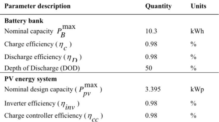
where DOD is the allowable depth of discharge given as a percentage. In this paper, the depth of discharge is assumed to be 50%. This DOD value is known to prolong the lifespan of the battery [17]. The data for the solar PV module and battery bank energy system are presented in Table 4.
Table 4: Solar PV module and battery bank energy storage system parameters
Parameter description Quantity Units
Battery bank
Nominal capacity PBmax 10.3 kWh
Charge efficiency ( c ) 0.98 % Discharge efficiency ( D ) 0.98 %
Depth of Discharge (DOD) 50 %
PV energy system
Nominal design capacity (Pmax
pv ) 3.395 kWp
Inverter efficiency (
inv
) 0.98 %
Charge controller efficiency (
cc
) 0.98 %
In this paper, the optimal operation of the hybrid energy system is investigated using two scenarios.
3.1.1 Scenario 1: Base case study
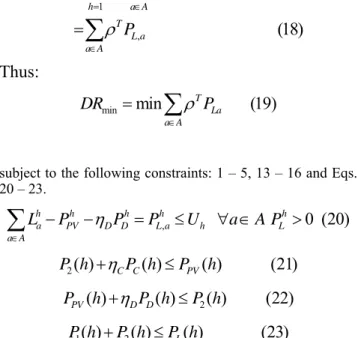
In this scenario, the DR optimization objective is to minimize the total daily electricity cost without considering the inconvenience cost of the residential customer, i.e, 0 0 , and is defined as in Eqn. 18
1 ,
(
)
(18)
H h h h h C a pv D D h a A T L a a AE
L
P
P
P
Thus:
minmin
(19)
T La a ADR
P
subject to the following constraints: 1 – 5, 13 – 16 and Eqs. 20 – 23. ,
0 (20)
h h h h h a PV D D L a h L a AL
P
P
P
U
a
A P
2( )
C C( )
PV( )
(21)
P h
P h
P
h
2( )
( )
( )
(22)
PV D DP
h
P h
P h
1( )
2( )
L( )
(23)
P h
P h
P h
3.1.2 Scenario 2: DR strategy with inconvenience cost
In Scenario 2, the DR optimization objective is to minimize both the total daily electricity cost and inconvenience cost of the residential customer, i.e, 0 1
,
. The optimization objective is formulated as in Eqn. 24 below.
0 , , 2 0 min , 0 , , , 1 1min
(24)
ah ah H H h h La La ah ah h a AhDR
P
P
CIC
subject to the following constraints: 1 – 5, 11 – 16 and Eqs. 20 – 23.
3. RESULTS AND DISCUSSION
All computations were carried out using Matlab software. In Fig. 4, the binary integer switching vector variables s07, s12,
s20 and s09, s14, s22, take the value 1 indicating the operation
time of cooker for scenarios 1 and 2 respectively.
Place Fig 4 here
The operation time of the cooker is shifted from s7 to s9, s12 to
s14 and s20 to s22 when DR optimization with inconvenience
cost for home appliance scheduling is applied. Figure 5 shows operation of TV for the different scenarios. The binary integer switching vector variable takes the value 1 at s08,09, s12,13 and
s22,23 for scenario 1 and s09,10, s14,15 and s20,21 for scenario 2.
The time of operation of the TV is shifted to the customer preferred end time during the day while in the evening the TV is shifted to start at the customer preferred starting time. On contrary, when DR optimization with inconvenience cost is applied, the operation time of TV during the day is shifted to customer preferred starting time and during the evening it is shifted further to the customer preferred end time.
Place Fig 5 here
The water boiler has flexible energy consumption levels and operates at different customer specified time intervals. It can be clearly seen from Figure 6 that the customer preference time intervals are not violated in the optimization models.
When DR optimization with inconvenience cost is applied, the respective energy consumption profiles of the water boiler are almost similar to scenario 1, between 0300hrs to 0600hrs and 1500hrs to 1600hrs. The energy consumption of the water boiler is higher at s07,12,20 and s09,14,17,18,19 in scenarios 1 and 2
respectively.
Place Fig 6 here
Figure 7 shows operation of vacuum cleaner for the different scenarios. The binary integer switching vector variable takes the value 1 at s10,11 and s21,22 for scenario 1 and
s11,12 and s20,21 for scenario 2. The time of operation of the
vacuum cleaner is shifted to 1100hrs and 1200hrs during the day while in the evening the vacuum cleaner is shifted to operate at 2000hrs and 2100hrs because of addition of the inconvenience cost to the DR optimization problem. The sequential operation of the vacuum cleaner can be clearly seen that it is not violated in all scenarios.
Place Fig 7 here
In Fig. 8, the electric vehicle is charged at different energy levels. From the figure, it can be clearly seen that the EV consumes more energy between 0100hrs to 0900hrs in all scenarios. During this time period both demand and cost is found to be less. The least energy requirement for the EV is at 2200hrs for both scenarios.
Place Fig 8 here
Table 5 below shows the total daily electricity cost for the residential customer for all the scenarios. The results show that different scenarios yield different total daily electricity cost for the residential customer.
Table 5: Total daily electricity consumption cost/bill of total home appliance load for different scenarios
Scenarios Total daily electricity cost (RSA)
Scenario 1 615.09
Scenario 2 621.97
In Figure 9, the power import from grid in scenario 2 has its first peak time occurring at 0700hrs as a result of three flexible home appliances all operating at this time, i.e., cooker, electric vehicle and water boiler. The second peak time for scenario 2 occurs at 2200hrs. At this time, in both scenarios, the water boiler is the only flexible appliance that is switched OFF. Much of the home appliance energy consumption is therefore coming from lights, TV, cooker, vacuum cleaner and electric vehicle. During this time the security lights are ON and therefore contributing to the total electricity consumption of the residential customer.The total daily electricity cost for scenario 2 is increased by about 1.1% when compared to scenario 1. Although there is an increase in cost the home appliance scheduling for flexible home appliances are in most cases starting at the preferred starting time of the residential customer. This point to the importance of inconvenience cost in DR optimization models for residential home appliance scheduling with flexible home appliances. The effect of flexible home appliances is very important to consider; however, it is also equally important not to shift all the home appliances to lower electricity tariff time periods without considering the inconvenience caused to the residential customer. By load shifting the flexible home
appliances during periods of higher electricity tariffs to the lowest electricity tariff periods the residential customer is able to save revenue. The use of TOU electricity tariffs therefore gives the opportunity for the residential customers to reduce their electricity cost through participating in DR strategies.
Place Fig 9 here
In Figure 10, the peak time for all scenarios occurs at 2100hrs and 2200hrs. The effect of solar PV module is clearly seen from the graph. During times when the solar radiation is not present, the power import from grid is high.
Place Fig 10 here
However, during the day, the power output of the solar PV module increases and in both scenarios, it is able to supply the energy consumption for all the home appliances. It can be seen that between 0100hrs to 0600hrs, the battery bank is able to supply power to all the home appliances for both scenarios. During the day, the solar PV module and battery bank storage system are able to supply the total appliance load between 1000hrs to 1900hrs for both scenarios. It can therefore be concluded that the use of solar PV module and battery storage bank have a significant effect on power import from the grid. Although the battery bank was able to supply the flexible home appliance between 0100hrs to 0400hrs, it was not enough to supply all the total energy requirement of all the home appliances for both scenarios between 0500hrs and 0800hrs. There is higher power import from grid for scenario 1 at 0800hrs before the solar PV module comes into effect. This was caused by the operation of water boiler and electric vehicle charging during this time. As the day progress, it can be seen that both the solar PV module and battery bank were able to cater for the total home appliance load for both scenarios. However, scenario 1 starts earlier at 0900hrs as compared to scenario 2 which starts at 1000hrs. During evening period, the battery bank in scenario 2 is able to supply the energy requirement of the home appliances until 2000hrs whereas for scenario 1 the battery bank only supplies the home appliance load until 1900hrs. The solar PV module was able to charge the battery bank between 0900hrs to 1700hrs and the stored energy was able to supply the excess energy requirement for the home appliances during sunset times
4. CONCLUSION
This paper presents the optimal operation of a hybrid energy system connected to the grid, incorporating DR strategy and inconvenience cost. The optimization problem of home appliance scheduling is presented as a mixed integer programming with a binary decision variable for switching home appliance ON and OFF. The optimization objective is to minimize both the total daily electricity cost and inconvenience cost of a residential customer with different time shiftable, power shiftable home appliances and customer preference constraints. The strategy of DR combined with inconvenience cost shows that it is important to schedule home appliances with the inconvenience cost incurred by the residential customer so that home appliances are not only shifted to the lower electricity tariff time periods but can also start at their customer preferred starting time. The results also show that the hybrid energy system is able to cater for all the energy requirements of home appliances during the day and this help to reduce the strain on the grid. This implies that solar PV
module power output and SOC of the battery bank are important parameters as it considerably affects the power flows of the hybrid energy system and the total electricity import from the grid. The results are important to both the residential customers and electricity suppliers, as they illustrate the optimal decisions considered in the presence of conflicting objectives. For residential customers, it can be used to balance the tradeoff between home appliance usage preferences and economic benefits. On the other hand, electricity suppliers can use the models to balance the tradeoff between electricity price and demand.
The analysis performed in this research work assumes that the residential customer follows the optimal home appliance schedule obtained by the model. However, this is not the case as the daily activities of the residential customer can be influenced by other factors like weather or other incentive schemes provided by the power utility. Thus, future work is on-going on designing a dynamic electricity pricing to include other incentive schemes that can better manage the demand response and ensure the stability of the power supply as may be influenced by renewable energy sources.
CONFLICT OF INTEREST
The authors declare that there is no conflict of interests regarding the publication of this paper.
ACKNOWLEDGEMENTS
This research is supported partially by South African National Research Foundation Grant (No. 112108) and South African National Research Foundation Incentive Grant (No. 95687).
REFERENCES
[1] Mckinsey on smart grid -sedc. [Available Online:] http://sedc-coalition.eu/wp-content/uploads/2011/06/mckinsey-10-08-05-smart -grid-benefits.pdf, 2011.(Accessed Nov 23, 2016)
[2] H. Aalami, G. Yousefi, M. Moghadam, Demand response model considering EDRP and TOU, in: IEEE PES, Transmission and Distribution Conference and Exposition, 2008, 21 - 24 April, Chicago IL.
[3] M. Malette, G. Venkataramanan, Financial incentives to encourage demand response participation by plug-in hybrid electric vehicle owners, IEEE Energy Conversation Congress and Exposition (ECCE), 2010, 4278 – 4284
[4] D. Setlhaolo, X. Xia, J. Zhang, Optimal scheduling of household appliances for demand response, Electric Power Systems Research,
2014, 116, 24 – 28.
[5] V. A. Evangelopoulos, P. S. Georgilakis, N. D. Hatziargyriou, Optimal operation of smart distribution networks: A review of models, methods and future research, Electric Power Systems Research, 2016, 140, 95 – 106.
[6] M. Erol-Kantarci, H. Mouftah, Wireless sensor networks for cost efficient residential energy management in the smart grid, IEEE Transactions on Smart Grid 1, 2011, 320 – 325.
[7] M. Song, K. Alvehag, J. Widen, A. Parisio, Estimating the impacts of demand response by simulating household behaviors
under price and CO2 signals, Electric Power Systems Research,
2014, 111, 103 – 114.
[8] D. Setlhaolo, X. Xia, Optimal scheduling of household appliances with a battery storage system and coordination, Energy and Buildings, 2015, 94, 61 – 70.
[9] O. Dzobo, X. Xia, Optimal operation of smart multi-energy hub systems incorporating energy hub coordination and demand response strategy, Journal of Renewable and Sustainable Energy, 2017, 9 (4), 045501
[10] O. Dzobo, K. Alvehag, C. T. Gaunt, R. Herman, Multi-dimensional customer segmentation model for power system reliability-worth analysis, International Journal of Electrical Power & Energy Systems, 2014, 62, 532 – 539.
[11] O. Dzobo, C. T. Gaunt, R. Herman, Reliability worth assessment of electricity consumers: a South African case study, Journal of Energy in Southern Africa, 2012, 23 (3), 31 – 39.
[12] O. Dzobo, C. T. Gaunt, R. Herman, M. J. Saulo, The effect of backup power supply on calculation of reliability cost and worth indices, in: Proceedings of the Third IASTED African Conference,
2010, vol. 684, pp. 032 – 128.
[13] O. Dzobo, C. T. Gaunt, R. Herman, Investigating the use of probability distribution functions in reliability-worth analysis of electric power systems, International Journal of Electrical Power & Energy Systems, 2012, 37 (1), 110 – 116.
[14] K. Alvehag, L. Söder, An activity-based interruption cost model for households to be used in cost-benefit analysis, in: Proceedings of Power Technology, 2007.
[15] R. Herman, C. T. Gaunt, Direct and indirect measurement of residential and commercial cic: Preliminary findings from South African surveys, in: Proceedings of the 10th International Conference on Probabilistic Methods Applied to Power Systems, PMAPS '08., 2008
[16] F. Fernandes, H. Morais, Z. VaZ., C. Ramos, Dynamic load management in a smart home to participate in demand response events, Energy and Buildings, 2014, 82, 592 – 606.
[17] P. Du, N. Lu, Appliance commitment for household load scheduling, IEEE Transactions on Smart Grid, 2011, 2, 411 – 419.
[18] H. Tazvinga, X. Xia, J. Zhang, Minimum cost solution of photovoltaic-diesel-battery hybrid power systems for remote consumers, Solar Energy, 2013, 96, 292 – 299.
[19] M. J. Morshed, A. Asgharpour, Hybrid imperialist competitive-sequential quadratic programming (hicsqp) algorithm for solving economic load dispatch with incorporating stochastic wind power: a comparative study on heuristic optimization techniques, Energy Conversion and Management, 2014, 84 30 – 40.
[20] G. J. Osorio, J. M. Lujano-Rojas, J. C. O. Matias, J. P. S. Catal, A probabilistic approach to solve the economic dispatch problem with intermittent renewable energy sources, Energy, 2015, 82, 949 – 959.
[21] V. S. Tabar, M. A. Jirdehi, R. Hemmati, Energy management in microgrid based on the multi objective stochastic programming incorporating portable renewable energy resource as demand response option, Energy, 2017, 118, 827 – 839.
[22] S. M. Nosratabadi, R. Allah Hooshmand, E. Gholipour, A comprehensive review on microgrid and virtual power plant concepts employed for distributed energy resources scheduling in power systems, Renewable Energy and Sustainable Energy Reviews, 2017, 67, 341 – 363.
[23] N. Good, K. A. Ellis, P. Mancarella, Review and classification of barriers and enablers of demand response in the smart grid, Renewable and Sustainable Energy Reviews, 2017, 72, 57 – 72.
[24] J. Wang, H. Zhong, Z. Ma, Q. Xia, C. Kang, Review and prospect of integrated demand response in the multi-energy system, Applied Energy, 2017, 202, 772 – 782.
[25] L. Swan, V. Ugursal, Modeling of end-use energy consumption in the residential sector: A review of modeling techniques, Renewable and Sustainable Energy Reviews, 2009, 13, 1819 – 1835.
[26] X. Xia, D. Setlhaolo, J. Zhang, Residential demand response strategies for South Africa, in: IEEE PES Power Africa 2012-Conference and Exhibition, 2012, 9 -13 July, Johannesburg, South Africa.
[27] P. Khajavi, H. Monsef, H. Abniki, Load profile reformation through demand response programs using smart grid, in: Proc. of the International Symposium on Modern Electric Power Systems, 2010, 20 – 22 September, Wroclaw, Poland.
[28] J. H. Yoon, R. Bladick, A. Novoselac, Demand response for residential buildings based on dynamic price of electricity, Energy and Buildings, 2014, 80, 531 – 541.
[29] K. Alvehag, L. S oder, Considering extreme outage events in
cost-benefit analysis of distribution systems, in: Proceedings of Australasian Universities Power Engineering Conference (AUPEC),

![Fig 2 shows the CIC of residential customers in Cape Town, South Africa used in this paper [15]](https://thumb-us.123doks.com/thumbv2/123dok_us/11087038.2995708/5.892.139.439.552.714/shows-residential-customers-cape-town-south-africa-paper.webp)