A Robust Panel Unit Root Test in the Presence of Cross Sectional Dependence

Volume 14 | Issue 2 Article 14

11-1-2015

A Robust Panel Unit Root Test in the Presence of

Cross Sectional Dependence

Nurul Sima Mohamad Shariff

Universiti Sains Islam Malaysia, [email protected]

Nor Aishah Hamzah

University of Malaya, Malaysia

Follow this and additional works at:http://digitalcommons.wayne.edu/jmasm

Part of theApplied Statistics Commons,Social and Behavioral Sciences Commons, and the

Statistical Theory Commons

Recommended Citation

Shariff, Nurul Sima Mohamad and Hamzah, Nor Aishah (2015) "A Robust Panel Unit Root Test in the Presence of Cross Sectional Dependence,"Journal of Modern Applied Statistical Methods: Vol. 14 : Iss. 2 , Article 14.

DOI: 10.22237/jmasm/1446351180

Dr. Shariff is a Lecturer with the Faculty of Science of Technology. Email her at

[email protected].

A Robust Panel Unit Root Test in the

Presence of Cross Sectional Dependence

Nurul Sima Mohamad Shariff

Universiti Sains Islam Malaysia Negeri Sembilan, Malaysia

Nor Aishah Hamzah

University of Malaya Kuala Lumpur, Malaysia

Problems arise in testing the stationarity of the panel in the presence of cross sectional dependence and outliers. The currently available panel unit root tests are very much affected by the presence of outliers. As such, this article introduces an alternative test which is robust to outliers and cross sectional dependence. The performance and robustness of the proposed test is discussed and comparisons are made to the existing tests via simulation studies.

Keywords: Cross sectional dependence, outliers, unit root, robust test, panel model.

Introduction

The investigation of the stationary in panel data has received great attention in panel analysis for the past few decades. It is an important issue in modeling the panel with the involvement of times series dimension in this study. This investigation can be done via unit root test. The panel unit root tests can be found in Im et al. (2003), Levin and Lin (1992, 1993), Levin et al. (2002), Bai and Ng (2004), Philips and Sul (2003), Moon and Perron (2004), Pesaran (2007) and Choi (2001, 2002). Hurlin (2010) distinguished two generations of unit root tests on which the first generation tests relied on the assumption that all cross sectional units are independent. The first generation of unit root tests were those proposed by Quah (1994), Breitung and Meyer (1994) and Levin and Lin (1992, 1993).

For the second generation of panel unit root tests, the presence of cross sectional dependence (hereafter CD) among the residuals is allowed within the panel. The assumption of CD is due to the evidence obtained on the strong co-movements among the economic variables (Barbieri, 2009). The assumption that the individual time series in the panel are cross sectional independent is not practical in the context of cross country regressions. As argued by O’Connell,

(1998), the presence of such CD may affect the finite sample behaviour of the panel unit root test which subsequently results to the incorrect decision in a unit root test. Those who proposed the tests which incorporated the CD were: Pesaran (2007), Philips and Sul (2003), Bai and Ng (2004), Moon and Perron (2004) and Choi (2002).

The existence of outliers implies that some shocks will only have temporary effects and thus, providing that they are sufficiently large or sufficiently frequent indicated that the series is stationary (Franses & Haldrup, 1994). Martin and Yohai (1986) showed via the simulation experiment that an additive outliers biases Ordinarily Least Squares (OLS) estimator downward for the parameter in a stationary first order autoregressive process. Hence, in some situations it could be expected that the additive outliers will establish the wrong impression that a time series is stationary when it is actually non-stationary. In addition, the presence of a cross sectional dependence may deteriorate the asymptotic distribution of the standard unit root test which is normally distributed (Philips & Sul, 2003; Banerjee, 1999). Due to such interest, a robust unit root test in the panel data model is proposed which aims at reducing the effects of outliers in the presence of the CD. Specifically, the presence of the unit root will be tested when both the CD and outliers exist in the panel. The finite sample behaviour of the proposed test is studied and its performance is evaluated through the Monte Carlo simulation study.

Model and Tests

Pesaran Unit Root Test

Specifically, in the presence of CD, the following model was considered by Pesaran (2007) to test the presence of the unit root:

1

;

1, 2, , .

1, 2, ,

it i i it i t it

y



b y

_



f



i

N t

T

  









(1)

where Δ

y

it =

y

it -

y

it-1;

y

it is an ith observation observed at a particular time t,

α

i is

the intercept, and

b

i is a parameter for the variable of

y

it-1. The presence of CD is

represented by

γ

i

f

t where

f

t is the latent factor and

γ

i is factor loadings that is common across cross sectional units i and



_it is the random error. This model can be employed for a larger and complicated set of time series. In the absence of the unit root, negative values for

b

i are expected. Specifically, the hypothesis test for a unit root is defined as follows:

0 1 : 0; for all 1, 2,..., : 0; for some 1, 2,..., i i H b i N H b i N     (2)

Rejecting the null explains that the panel is stationary (no unit root). Model (1) can be expressed as cross sectional Augmented Dickey-Fuller (CADF) model:

1 1

;

1, 2, , .

1, 2, ,

it i i it i t i t it

y



b y

_

c y

_

d y

e

i

N t

T

  



  





(3)

where the standard of Augmented Dickey-Fuller (ADF) model is improved up to more variables in independent variables in model (3), that are; cross section averages of lagged levels (

y

_t1) and first differences of the individual series (



y

_t ),

i in the model. Pesaran has shown that the effect of CD can be eliminated by using model (3). Thus, let CADFi be the ADF statistics for the ith _{cross sectional unit}

given by the t-ratio of the OLS estimate

b

ˆ

_i of

b

i in the CADF regression (3). Then, the Pesaran unit root test is given by

1 CADF CIPS N i i N  



(4)

where CIPS stands for cross sectional augmented IPS (Im et al. (1997) unit root test) . This CADFiis given by



 







1 , 1 , 1 , 1 1 2 , 1 , 1 CADF ( , ) T T i i i i i i T i i i t N T            y My y M y y My (5) where y_{i, 1} 



y_i1, ,y_iT₁



T ,



2, 3, ,



T i yi yi yiT   y   ; 2 2 1 ˆ 4 it T t i e T



_  



,with

ˆ

_{it it}

ˆ

_it

e

   

y

y

and M is defined as



T



1 T t    M I H H H H and

H

 

( ,

1 y y

_t

,

_t₁

)

. t

I

is a unit matrix of order

T T



and H is the combination of the dummy variables, average of cross section of the first difference of

y

it and its first lagged value

y

it-1. The asymptotic distribution of this distribution is more skewed

compared to the ADF (asymptotically normal) distribution in the presence of CD (Philips and Sul, 2003). The critical value of the test statistics in (5) is given in

Table 1 and those are obtained from the simulation experiment based on the CADF model.

Proposed Unit Root Test

The Pesaran’s unit root test uses the OLS procedure that is non-robust. It has been known in the literature that the OLS is sensitive to the influence of outliers in the data. Hence, to limit the influence of outliers in the data in investigating the presence of the unit root in the model, the Generalized M-estimator is applied and it is obtained by solving the following equation:



1

 

1



 

_

_

1 1 1 ˆ 0; for 1, 2, , ˆ T it i i it i it i it t i i it e b u y v y y i N v y                 



(6) where

u y

_i

 

_it1



1

and









1 1 1 . i it it v y d y  

 The

d y

 

_it1 is given as a measure of the outlying the

y

it-1 in the X-space from its mean value. Here,

ψ

i (.) is the derivative

of

ρ

i (.), where

ρ

i (.) is a differential convex function (with minimum at 0) and is known as the robustifying criterion function while

e

ˆ

it

 

b

i is the estimated residuals and



ˆ

_i is the robust scale obtained from the first iteration of M-estimation.

To test for a unit root, a similar hypothesis statement as in (2) is considered. Under H0 of no unit root, the generalization of the test is given by:

ˆ ˆ ( ) i i i i b b t Var b      (7) where ˆ i

b is the Generalized M-estimator where it is computed as follows:



 

1



, 1 , 1 , 1 ˆ i T T i i i i i i b  y G y   y Gy (8)

where y_{i, 1} 



y_i1, ,y_iT1



T ,   y_i



y_i2,y_i3, ,y_iT



T and

G

_i



M W

 _i

 

z

_it

with



₁

  

ˆ ˆ it i it i it i e b z d y



  . The ( )ˆ i Var b is given by





 





 





2 1 ₂ 1 , 1 , 1 2 1 ˆ ˆ ˆ _ˆ ( ) . ˆ ˆ i it i i i i it T i i i it i i i i it e b E v y Var b e b E v y                    _{ }          _  _  _{  }   y M y (9)

where

E





_i

 

.



and E



_i,

 

.



are the expected values of robustifying criterion function



i

 

.

and derivative of



i

 

.

, respectively. The

 M is computed as





1 T T t   _{ }    

M I H H H H ;

I

_t is an identity T by T matrix and

   



,



y

t 1

,



y

t











H

1

. The value of



 

.

in Htakes the form

 

 





 

1 1 1 1 1 1 1 ,if median , , ,elsewhere and t t t t t Nt i t t y y c y sign y y y y y                  

 



1



,if median , , ,elsewhere t t _i t Nt y d sign y y y           (10)

where c and d are the critical values and computed as 1

ˆ

3

t y



_ and

3

ˆ

t y



_ , respectively. The 1

ˆ

t y



_ and

ˆ

t y



_ are robust scale with

 

1 1 1 ˆ 1.4825 median median , t y t t t y t y



_  _  _

 

ˆ 1.4825 median median t y t t t y t y



_     , respectively. These robust scales are

chosen to achieve specified level of efficiency and are called as the Median Absolute Deviation (MAD) with the tuning constant 1.4825 where

1

ˆ

t y



_ and

ˆ

t y



_

are consistent for

σ

at the normal distribution.

1 RCIPS i i N i t t N     



(11) where

t

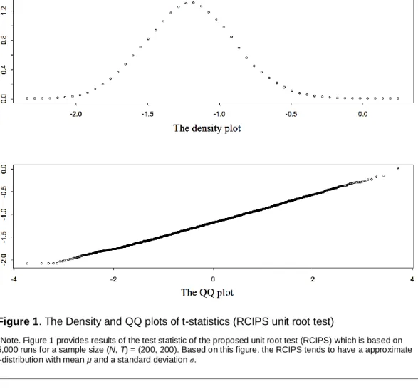
_i is given in (7).

The asymptotic distribution of the test statistics given in (7) is obtained through the extensive simulation experiment. Based on Figure 1, the RCIPS unit root test tends to have an approximate t-distribution with a mean

μ

and a standard deviation,

σ

. As the sample size increase, it is believed that the RCIPS will approach to a standard normal distribution. This result is comparable with Pesaran (2007) under conditions where

e

it is normally distributed.

To investigate the performance of the RCIPS, the critical region of test statistics is required. Therefore, the critical region of RCIPS test is obtained through simulation experiment at the 0.05 level of significance and it is given in Table 2. The data generating process (DGP) and results are given in the next section.

Finite Sample Behavior of the Tests

Following Pesaran (2007), the following DGP is considered:

1

(1

)

it i i i it it

y







 



y

_



e

;

e

_it





_iT

f

_t





_it ;



_i

~

iidN

(0,1)

;



_it

~

iidN

(0,



_i2

)

;





2

~

0.5,1.5 .

i

iidU



The presence of CD is characterized by the latent factor

f

t ~ iidN(0, 1) and strong CD,

γ

i ~ iidU (0.5, 1.5). The performance of the tests is measured by setting: 1)

φ

i = 1 and 2)

φ

i ~ U [0.75, 0.95] for computing the size (incorrect detection) and power (correct detection) of the test, respectively.

A panel contaminated by outliers is represented by

y

_it



y

_it





 

L



I

_it

 



for i = 1, 2, …, N. t = 1, 2, …, T, where

y

_it is the observed contaminated series,

y

it is the uncontaminated series, ξ (L) is the dynamic pattern of the outliers, ω is the magnitude of outliers.

I

it (τ) is the indicator function of the presence of outlier and will takes the value of 1 at time t = τ (chosen at random) and 0 elsewhere.

Figure 1. The Density and QQ plots of t-statistics (RCIPS unit root test)

*Note. Figure 1 provides results of the test statistic of the proposed unit root test (RCIPS) which is based on 5,000 runs for a sample size (N, T) = (200, 200). Based on this figure, the RCIPS tends to have a approximate t-distribution with mean μ and a standard deviation σ.

Two types of outliers are considered in this study; additive outliers (AO) and temporary change (TC). The AO only affect the level but leave the variance unaffected. The TC will produce an abrupt step and dies out gradually in time. Hence, in

y

_it ,



 

L



1

in the presence of AO and TC takes the form of

 

1 1 L L   

 where δ represents the velocity of the dynamic effect and is bounded

by [0, 1] (Tsay, 1998). The performance of the tests is investigated at the 5% level of significance using the sample sizes N = (20, 30, 50) and

Results and Discussion

The size and power of the unit root tests are investigated for the uncontaminated panel, the panel with AO and the panel with TC. These are tabulated in Tables 3 to

4 for the size and power of the tests, respectively. The results of the tests are reported by rows: 1) CIPS and 2) RCIPS with three columns of the number of cross sectional units, N = (20, 30, 50). For each column of N = (20, 30, 50), results of the size and power of the unit roots tests are reported when the panel is 1) uncontaminated, 2) contaminated with AO, and 3) contaminated with TC.

In the uncontaminated panel, the CIPS unit root test gives a smaller size for a small sample but attains a reasonable size as T increases whereas the RCIPS is slightly oversized even when N and T are large. In the presence of the AO and TC, the sizes for the CIPS test are all zeros for all sample sizes. The RCIPS has smaller size in the presence of AO but achieves a good size of the test in the presence of TC compared to CIPS. These results are comparable when the panel is free from the outliers effect (see column of “no cont” of Table 3).

In investigating the power of the test in the uncontaminated panel, the CIPS gives slightly lower correct detection (power) of a unit root for T ≤ 50. The probability of correctly detect the presence of unit root however increasing (good power) as T increases and the result is comparable to those obtained in Pesaran (2007). The RCIPS outperforms the CIPS even for small sample. In the presence of the AO and TC the panel, the powers for the CIPS test are poor when T ≤ 50. The power however increases for T ≥ 100 with an increasing N. The powers for both tests are good as N increases in the presence of TC in the panel. The RCIPS provides a sensible power when T ≤ 30 in the presence of the AO but outperforms the CIPS in the presence of the TC. Based on these results, the RCIPS provides a good reasonable size (close to 0.05) and power (greater than 0.95) in the presence of the AO and TC relative to CIPS especially when N and T are small.

Conclusion

An alternative approach to Pesaran unit root test is proposed in order to investigate the stationarity of the data when outliers occur in the panel. The proposed test is robust to the effect of spurious observation in data. The finite sample behaviour of the tests is studied and compared via the Monte Carlo experiments. The results show that the proposed unit root test provide comparable size and power of the test in uncontaminated panel and yield better results than Pesaran unit root test in the presence of outliers in the panel especially for the small pair of sample size.

Table 1. Critical Values of CIPS N 20 30 50 Level of significance / T 1% 5% 10% 1% 5% 10% 1% 5% 10% 20 -2.40 -2.21 -2.10 -2.32 -2.15 -2.07 -2.25 -2.11 -2.03 30 -2.38 -2.20 -2.11 -2.30 -2.15 -2.07 -2.23 -2.11 -2.04 50 -2.36 -2.20 -2.11 -2.30 -2.16 -2.08 -2.23 -2.11 -2.05 100 -2.36 -2.20 -2.11 -2.30 -2.16 -2.08 -2.23 -2.12 -2.05 200 -2.36 -2.20 -2.11 -2.30 -2.16 -2.08 -2.23 -2.12 -2.05

These results are quoted from Pesaran (2007). The critical values are obtained from the estimates of

  

Y

_it



_i

bY

_{i it}₁

  

c Y

_{i t}

d Y

_{i t}₁



e

_it with the test statistic is

given by regression based on 10,000 runs. The test statistic is given by

1

/

i i N i

t

t

N







(the details of this expression can be referred in equation (5)) and the results of the test statistics are reported at 1%, 5% and 10% level of significance.

Table 2. Critical Values of RCIPS

N 20 30 50 Level of significance / T 1% 5% 10% 1% 5% 10% 1% 5% 10% 20 -1.6240 -1.3834 -1.2711 -1.5179 -1.3423 -1.2458 -1.4291 -1.2888 -1.2124 30 -1.6565 -1.4592 -1.3637 -1.6139 -1.4300 -1.3319 -1.5264 -1.3843 -1.2931 50 -1.7569 -1.5555 -1.4484 -1.6979 -1.4987 -1.4138 -1.6126 -1.4483 -1.3692 100 -1.8267 -1.6090 -1.5238 -1.7662 -1.5894 -1.6866 -1.6866 -1.5242 -1.4575 200 -1.8983 -1.6946 -1.5992 -1.8397 -1.6613 -1.5646 -1.7706 -1.6182 -1.5319

Following the work of Im et al. (2003), the DGP computing critical values for RCIPS test is given by

y

it



y

it1



e

it

,

with

e

it

~

iidN

(0,1)

; for

i = 1, 2, …, N. t = 1, 2, …, T based on 5,000 runs. The test statistic is given by

1

/

i i N i

t



t



N







(the details of this expression can be referred in equation (11)) and the results of the test statistics are reported at 1%, 5% and 10% level of significance.

Table 3. The size of the unit root tests CIPS no cont AO TC no cont AO TC no cont AO TC T/N 20 30 50 20 0.006 0.000 0.000 0.003 0.000 0.000 0.006 0.000 0.000 30 0.011 0.000 0.000 0.004 0.000 0.000 0.002 0.000 0.000 50 0.012 0.000 0.000 0.014 0.000 0.000 0.009 0.000 0.000 100 0.047 0.000 0.000 0.022 0.000 0.000 0.028 0.000 0.000 200 0.034 0.000 0.008 0.035 0.000 0.000 0.025 0.000 0.000 RCIPS no cont AO TC no cont AO TC no cont AO TC T/N 20 30 50 20 0.041 0.008 0.039 0.058 0.006 0.038 0.056 0.004 0.056 30 0.074 0.013 0.042 0.042 0.011 0.023 0.062 0.002 0.045 50 0.053 0.004 0.030 0.049 0.026 0.032 0.059 0.021 0.054 100 0.076 0.048 0.051 0.078 0.073 0.045 0.074 0.052 0.039 200 0.069 0.081 0.042 0.057 0.076 0.052 0.080 0.073 0.044

The values are the probability of rejecting the null of a unit root based on 1000 replications in uncontaminated panel (column no cont), contaminated with AO (column AO) and contaminated with TC (column TC). The size (probability of rejecting the null of a unit root when the unit root is present in the data) of the test is computed for

φ

i = 1. The H0 is rejected if the respective test statistics is greater

Table 4. The Power of the unit root tests CIPS no cont AO TC no cont AO TC no cont AO TC T/N 20 30 50 20 0.002 0.000 0.000 0.022 0.000 0.000 0.018 0.000 0.000 30 0.207 0.000 0.000 0.241 0.000 0.000 0.283 0.000 0.001 50 0.862 0.011 0.026 0.952 0.005 0.023 0.999 0.007 0.022 100 1.000 0.918 0.836 1.000 0.282 0.955 1.000 0.355 0.977 200 1.000 0.981 1.000 1.000 0.993 1.000 1.000 1.000 1.000 RCIPS no cont AO TC no cont AO TC no cont AO TC T/N 20 30 50 20 0.793 0.422 0.788 0.912 0.481 0.833 0.952 0.683 0.961 30 0.920 0.617 0.865 0.964 0.755 0.965 0.981 0.804 0.980 50 0.994 0.834 0.968 1.000 0.922 0.988 1.000 0.986 1.000 100 1.000 1.000 1.000 1.000 1.000 1.000 1.000 1.000 1.000 200 1.000 1.000 1.000 1.000 1.000 1.000 1.000 1.000 1.000

The values are the probability of rejecting the null of a unit root based on 1000 replications in uncontaminated panel (column no cont), contaminated with AO (column AO) and contaminated with TC (column TC). The power (probability of correctly rejecting the null of a unit root when the unit root is absence in the data) of the test is computed for

φ

i ~ U [1.75, 0.95]. The H0 is rejected if the respective

test statistics is greater than theirs critical values (tabulated in Tables 1 and 2) at 5% level of significance.

Acknowledgments

The authors gratefully acknowledge the helpful comments from the participant at the International Conference on Computing, Mathematics and Statistics 2013 held in Bay View Beach Resort, Penang, Malaysia and the grant support USIM/ERGS-FST-33-50312from the Universiti Sains Islam Malaysia (USIM), Malaysia.

References

Bai, J. & Ng, S. (2004). A PANIC attack on unit roots and cointegration.

Econometrica, 72(4), 1127-1177.

Banerjee, A. (1999). Panel data unit root and cointegration: An overview.

Oxford Bulletin of Economics & Statistics, 61(S1), 607-629. doi:10.1111/1468-0084.0610s1607

Barbieri, L. (2009). Panel unit root tests under cross-sectional dependence: An overview. Journal of Statistics: Advances in Theory and Applications, 1(2), 117–158.

Breitung, J. & Meyer, W. (1994). Testing for unit roots in panel data: Are wages on different bargaining levels cointegrated? Applied Economics, 26(4), 353-361. doi:10.1080/00036849400000081

Choi, I. (2001). Unit root tests for panel data. Journal of International Money and Finance, 20(2), 249-272. doi:10.1016/S0261-5606(00)00048-6

Choi, I. (2002). Combination Unit Root Tests for Cross-Sectionally Correlated Panels. Mimeo, Hong Kong University of Science and Technology.

Franses, P. H. & Haldrup, N. (1994). The effects of additive outliers on tests for unit roots and cointegration. Journal of Business and Economic Statistics,

12(4), 471-478. doi:10.1080/07350015.1994.10524569

Hurlin, C. (2010). What would Nelson and Plosser find had they used panel unit root tests? Journal of Applied Economics, 42(12), 1515-1531.

doi:10.1080/00036840701721539

Im, K. S., Pesaran, M. H., & Shin, Y. (1997). Testing for Unit Roots in Heterogenous Panels. DAE, Working Paper 9526, University of Cambridge.

Im, K. S., Pesaran, M. H. & Shin, Y. (2003). Testing for Unit Roots in Heterogeneous Panels. Journal of Econometrics, 115(1), 53-74.

doi:10.1016/S0304-4076(03)00092-7

Levin, A. & Lin, C. F. (1992). Unit Root Test in Panel Data: Asymptotic and Finite Sample Properties. University of California at San Diego, Discussion Paper. 92-93.

Levin, A. & Lin, C. F. (1993). Unit Root Test in Panel Data: New Results. Discussion Paper No 93-56. Department of Economics, University of California at San Diego.

Levin, A., Lin, C. F. & Chu, C. S. J. (2002). Unit root tests in panel data: Asymptotic and finite-sample properties. Journal of Econometrics, 108(1), 1-24. doi:10.1016/S0304-4076(01)00098-7

Martin, R. D. & Yohai, V. J. (1986). Influence functionals or time series.

The Annals of Statistics, 14(3), 781-818. doi:10.1214/aos/1176350027

Moon, H. R. & Perron, B. (2004). Testing for a unit root in panels with dynamic factors. Journal of Econometrics, 122(1), 81-12.

doi:10.1016/j.jeconom.2003.10.020

O’Connell, P. (1998). The overvaluation of purchasing power parity.

Journal of International Economics, 44(1), 1-19. doi:10.1016/S0022-1996(97)00017-2

Pesaran, M. H. (2007). A simple panel unit root test in the presence of cross section dependence. Journal of Applied Economics, 22(2), 265-312.

doi:10.1002/jae.951

Philips, P. C. B. & Sul, D. (2003). Dynamic panel estimation and

homogeneity testing under cross section dependence. Econometrics Journal, 6(1), 217-259. doi:10.1111/1368-423X.00108

Quah, D. (1994). Exploiting cross-section variation for unit root inference in dynamic data. Economics Letters, 44(1-2), 9-19.

doi:10.1016/0165-1765(93)00302-5

Tsay, R. S. (1998). Outliers, level shift, and variance changes in time series.