Statistical methods for modeling RNA-Seq short-read data

(1)

STATISTICAL METHODS FOR MODELING RNA-SEQ SHORT-READ DATA

BY

DAVID DALPIAZ

DISSERTATION

Submitted in partial fulfillment of the requirements for the degree of Doctor of Philosophy in Statistics

in the Graduate College of the

University of Illinois at Urbana-Champaign, 2014

Urbana, Illinois

Doctoral Committee:

Associate Professor Ping Ma, Chair, Director of Research Professor Jeffrey Douglas

Professor Douglas Simpson

(2)

Abstract

This thesis explores various methods for analyzing data generated using the next-generation sequencing technology, RNA-Seq. Two methods are developed which at-tempt to accurately calculate RNA expression, the first using a penalized regression approach to remove bias based on nucleotide composition, as well as a second which demonstrates the use of variation as an estimate of gene expression. Another method is developed which utilizes RNA-Seq gene expression data to identify genomic regu-latory elements using a semi-parametric model with multiple responses considered si-multaneously. Lastly, a method is established which identifies differentially expressed genes in timecourse data using a functional ANOVA mixed-effect model.

(3)

Acknowledgements

First and foremost I would like to thank my committee members Jeffery Douglas, Ping Ma, Douglas Simpson and Wenxuan Zhong for working with me during this process. A special thanks to my advisor Ping for guiding me through the last four years. Funding for this work has come from the grants of Ping and Wenxuan which include NSF 0800631, 1055815, 1120256, 1222718, and DMS-1228288. Additionally thanks to Han Wu and Xiaoxiao Sun for their assistance and guidance in creating data for this work. I would also like to express my appreciation for all of the help provided by Melissa Banks during my time with the Department of Statistics. Lastly, I would like to thank my friends and family for their support over the years.

(4)

Chapter 1 Introduction

1.1 RNA-Seq Short-Read Data

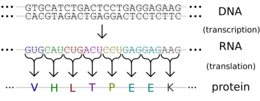
The central dogma of molecular biology, stated in Cricket al.(1970), explains each of the possible avenues for information transfer in biological systems. Specifically it de-scribes the ways in which information flows between the three major macromolecules which are essential for life: deoxyribonucleic acid (DNA), ribonucleic acid (RNA), and finally proteins. Figure 1.1 outlines five of these nine possible information transfers. Transfers from DNA to DNA, DNA to RNA, and RNA to protein are considered the group of general transfers. These general transfers are referred to as DNA replication, transcription and translation respectively. The special transfer of RNA to DNA is called reverse transcription and is an important step in the creation of data in this work.

Many of the methods developed in this thesis are centered around the biological process of gene expression which is shown in Figure 1.2. The most basic definition of gene expression is used to attribute a particular phenotype to a particular geno-type. The genotype is defined by the genome of an organism which is encoded using DNA. DNA, deoxyribonucleic acid, is composed of four nucleotides adenine, cytosine, thymine, and guanine. These are notated using A, C, T and G. DNA is composed of two strands of these nucleotides arranged in a double helix. The nucleotides, also called base pairs, are connected between the two strands according to pairing rules, specifically, A goes with T and C goes with G, so the information of the genome is

(7)

Figure 1.1: The central dogma of biology. The central dogma of biology, from Crick et al. (1970) establishes the possible information transfers in biology. Shown here are the general transfers; DNA replication (DNA to DNA), transcription (DNA to RNA), and translation (RNA to protein). Also shown are two special trans-fers; reverse transcription (RNA to DNA) and RNA replication (RNA to RNA). Reverse transcription plays an important role the next-generation sequencing tech-nology RNA-Seq.

(8)

Figure 1.2: Gene expression. Gene expression shown via both transcription to RNA as well as translation to protein.

known through a single strand. Specific sections of the genome, various lengths of sequences of A, C, T and G, are labeled genes. The term gene has many associated definitions but for the purpose of this work a section of the genome which is used to create a gene product will be labeled a gene. Gene product may be either RNA or ultimately protein. Stretches of DNA sequences which are not considered genes are sometimes called “junk DNA.” A more appropriate term is non-coding DNA. While some DNA may truly serve no purpose, however this seems increasingly unlikely, some non-coding DNA is currently known to serve a number of functions. One in particular which will be discussed in Chapter 4 is regulation through the use of transcription factor binding sites.

The genetic code which makes up the genotype determines the phenotype. Specif-ically, genes are used to create RNA and then protein, which are both gene products. The process of creating RNA or protein from the corresponding genes is called gene expression. The process of creating RNA copies from the DNA of a gene is referred to as transcription. Transcription takes place in a cell nucleus using RNA polymerase. The RNA polymerase reads the DNA sequence one nucleotide at a time and simul-taneously adds the corresponding RNA nucleotide to a newly created RNA strand. While DNA uses the nucleotides adenine, cytosine, thymine, and guanine, RNA in-stead uses guanine, adenine, uracil and cytosine which are notated using G, A, U and

(9)

C. So DNA nucleotides A, C and G become RNA nucleotides A, C and G. The DNA nucleotide T is replaced by an RNA nucleotide U.

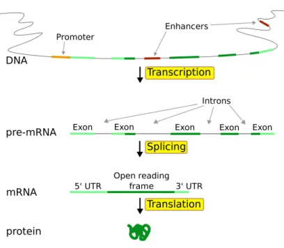
The initial transcription step transfers all of the coding DNA of a particular gene while nearby non-coding DNA such as promoters are left out. Before translation to protein, eukaryotic organisms require a second RNA processing step called splicing, which is shown in Figure 1.3. The product of the initial transcription is called pre-mRNA which contains two distinct type of sequences, namely introns and exons. The sequences labeled introns will be removed during splicing, while sequences labeled exons are retained during splicing and join to create messenger RNA, mRNA. (The definitions of intron and exon and based on their retention or removal during splicing. While introns are removed before the creation of mRNA they are still believed to have other biological functions.) Before splicing the RNA content may be called the transcriptome, while after splicing it is referred to as the exome. The mRNA sequence produced from the DNA of a particular gene may also be referred to as a gene to indicate it came from a particular sequence of DNA.

The final gene product, protein, is created from mRNA via translation. Certain exons of the final mRNA are considered part of the coding sequence and are used for translation into protein. Others, at either end of the sequence are part of the untranslated region. (This distinction can be used to label exons as coding and non-coding.) The coding sequence of RNA nucleotides is considered in triplets called condons such as UUU, UCA, GAC, and so on. Each codon is translated into a particular amino acid, the combination of which makes up the final protein.

Quantifying gene expression is a common task in biology research. Researchers would ultimately like to measure the final gene product, protein, but this is currently a difficult task. The much easier and more common measurement is that of mRNA. Numerous methods exist for measuring mRNA. RT-qPCR, or reverse transcription quantitative polymerase chain reaction can be used to to measure the number of

(10)

Figure 1.3: From DNA to Protein. Details of the gene expression process including the splicing step.

copies of known mRNA sequences. DNA microarrays can be used to simulataneously measure the relative mRNA abundance of a number of known genes.

RNA-Seq is a high-throughput sequencing technology which is used to investi-gate the RNA content of a sample by sequencing its cDNA. (Wang et al. (2009)) RNA-Seq is sometimes referred to as “next-generation sequencing” and is the current successor to DNA microarrays for sequencing the entire transcriptome. Unlike mi-croarrays, RNA-Seq can be used to provide nucleotide level information for the entire transcriptome, thus making it a powerful tool for transcriptomics.

RNA-Seq data creation begins with gathering a sample of RNA which is then used to produce a cDNA fragment library. This cDNA library is obtained through the use of the previously mentioned reverse transcription which transfers information from the RNA of the sample to cDNA. (cDNA, complementary DNA, is the name given to DNA which has been synthesized from RNA using reverse transcription.) Each of these cDNA fragments are then sequenced to obtain “short-reads.” A “short-read”

(11)

refers to the nucleotide composition of the sequence. RNA molecules are composed of four nucleotides: guanine, adenine, uracil and cytosine. These are notated using G, A, U and C. However, since RNA-Seq uses reverse transcription, “short-reads” are always written using the corresponding DNA nucleotides which are adenine, cytosine, thymine, and guanine. These nucleotides are notated using A, C, T and G. (Often reference will be made to base pairs (bp) which comes from the double-stranded nature of DNA despite the single stranded nature of cDNA and mRNA.) For example, the sequence AATGCTCGTTAGCTAGTCGATGGCC, is a “short-read” of length 25. Frequently, RNA-Seq analysis focuses specifically on messenger RNA (mRNA) which is used for translation into amino acids and thus the creation of protein. Several methods exist for mRNA isolation of RNA samples. (Aranda IV et al.(2009))

Currently this sequencing is done using a number of sequencing technologies in-cluding the Illumina Genome Analyzer IIx, Applied Biosystems SOLiD and Roche 454. Read length can vary from roughly 30-400 base pairs, before trimming based on quality scores. After obtaining millions of short-reads from sequencing, these reads are mapped (or “aligned”) to a reference genome or reference transcripts. (Or used to obtain a de novo assembly, which will not be considered in this text but is a con-siderable advantage over the previous microarray technology.) A number of software packages exist for read mapping, including Bowtie, SeqMap, Short Oligonucleotide Analysis Package (SOAP), and CLC Genomics. Once the reads have been mapped, relative abundance can be used to determine RNA gene expression levels. The most commonly used method of quantifying gene expression, RPKM developed in Mor-tazavi et al. (2008), is used to correct for two well known biases. RPKM, or reads per kilobase per million mapped reads, is the number of reads mapping to a partic-ular gene, normalized both by the length of the gene, as well as the total number of mapped reads over the entire genome. Correcting for the length of gene and total mapped reads allows for comparison between genes within an experiment, as well as

(12)

comparison of the same gene between experiments, respectively.

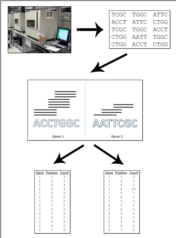
Figure 1.4 details the data creation process, which is necessary before embarking on statistical analysis. Again, using a sample of RNA, short-reads are obtained. At this point there are essentially two steps remaining before statistical analysis, mapping and storing the data for analysis.

For the majority of the following chapters, the data has been mapped to the reference using the alignment tool Bowtie. (Langmead et al. (2009)) At the most basic level, each short-read is compared with each possible position on the genome and checked for matching nucleotide composition. (The actual algorithms used in practice are much more efficient.) More specifically, there are a number of options for how we determine the alignments. An alignment is a combination of a short-read (sequence of A, C, T and G) and a position on the reference genome. (Where each nucleotide of the read matches the reference.)

First, there are a number of options determining what is a valid alignment. It is possible to define a valid alignment as those where the read exactly matches the reference. For practical reasons however, this is usually not the case. In practice valid alignments maybe be allowed to contain a limited number of mismatches with the reference. This will allow for reads with sequencing errors to still be mapped. This also allows for alignment given the presence of genetic variation such as a single-nucleotide polymorphism. There are a number of metrics for allowing mismatches, all of which are detailed in the Bowtie documentation. (Frequently a small number of mismatches, usually between one and five depending on the read length, are allowed, as long as their combined quality scores do not exceed a predetermined threshold. This would mean they are all rather unlikely to truly be mismatched.)

Second, it must be decided which alignments are reported. There are generally a number of ways to do this, arising from the fact that with current read lengths, there are frequently reads with multiple valid alignments. The default behavior of

(13)

the Bowtie aligner is to simply output the first valid alignment for a read, and not consider any further alignments. While this is by far the fastest method, it is not frequently used. One method, after finding all possible valid alignments, simply reports them all. (Methods for estimating gene expression which rely on this type of data probabilistically assign the reads with multiple reported alignments.) Another method only reports alignments with one valid alignment. A middle-ground between reporting all valid alignments and uniquely aligning reads, would be to first find all valid alignments, then report the best alignment based on quality scores. Each of these methods are currently used in practice with the unique method seemingly the most popular.

Once a list of reported alignments has been created, that data is converted into a format which will be used for statistical analysis by summarizing the alignments at each nucleotide. The bottom two images of Figure 1.4 illustrate two ways this may be done. The first lists read counts at each nucleotide position determined by the number of reads which begin at that particular position. The second, instead of only considering the start positions, lists the number of reads that cover each position. (Either of these can be used to obtain a simple count of the total number of reads mapping to a gene which could then be used to calculate simple expression estimates such as RPKM.) While both of these methods are used in practice, it is frequently more beneficial to have data based on the starting position of the reads.

1.2 Chapter Descriptions

• Chapter 2: Bias Correction in RNA-Seq Short-Read Counts using Penalized

Regression includes work which appeared in Statistics in Biosciences in 2012 along with Ping Ma and Xuming He. A penalized regression approach is used to remove bias in RNA-Seq short-read counts based on the information of the

(14)

Figure 1.4: RNA-Seq data creation process. An illustration of two ways to conceptualize RNA-Seq data. Top Left: Physical samples are sequenced. Top Right: Output of sequencing, a series of short-reads. Middle: The sequenced reads are mapped to the genome. Here for example the example reads are mapped to two example genes. Bottom Left: First data conceptualization. The mapped reads are stored according to the start position of their mapping. Bottom Right: Second data

(15)

surrounding nucleotides of a given read in a computationally efficient manner.

• Chapter 3: Gene Expression Quantification Using Transcript Reads Variation

includes work with Ping Ma which introduces a novel approach to estimating gene expression levels based on a mixture of mean and variance rather than only the mean of the read counts. Preliminary results were presented at the 2012 Joint Statistical Meetings.

• Chapter 4: Identification Of Regulatory Elements Using Next-Generation

Se-quencing Datais work with Wenxuan Zhong. We develop a method for identify-ing regulatory elements usidentify-ing a semi-parametric model with multiple responses considered simultaneously. Preliminary results were presented at the 2012 Al-gorithms for Threat Detection Workshop.

• Chapter 5: Identifying Differentially Expressed Genes Using Timecourse

RNA-Seq Short-Read Count Data is work with Ping Ma to identify differentially expressed genes using timecourse RNA-Seq read count data. The proposed method uses a functional ANOVA mixed-effect model and a test is developed based on the resulting Kullback-Leibler ratio.

(16)

Chapter 2 Bias Correction in RNA-Seq

Short-Read Counts using Penalized

Regression

RNA-Seq produces tens of millions of short reads. When mapped to the genome or reference transcripts, RNA-Seq data can be summarized by a very large number of short-read counts. Accurate transcript quantification, such as gene expression calculation, relies on proper correction of sequence bias in the RNA-Seq short-read counts. We use a linear model for the sequence bias, which is much more flexible than the popular Poisson model. We fit the model using a penalized regression method, which allows for a significant dimension reduction. The algorithm is scalable for modeling RNA-Seq data. We demonstrate the excellent performance of the proposed method by applying it to real data examples. The methods are implemented in open-source code, which is available in the R packagelmbc.

2.1 Introduction

With the rapid development of second-generation sequencing technologies, RNA-Seq has become a popular tool for transcriptome analysis (Mortazavi et al. (2008), Na-galakshmiet al. (2008), Wilhelm et al.(2008)). It produces digital signals and offers the chance to detect novel transcripts by obtaining tens of millions of short reads. When mapped to the genome or reference transcripts, RNA-Seq data can be summa-rized by a tremendous number of short-read counts. The huge number of short-read counts enables researchers to make transcript quantification in ultra-high resolution. A number of researchers have worked on transcript quantification, in particular,

(17)

the gene expression calculation, using these short-read counts. Mortazaviet al.(2008) develop a simple method, in which the expression level of a transcript is quantified as reads per kilobase of the transcript per million mapped reads to the transcriptome (RPKM). A variant, FPKM is developed in Trapnell et al. (2010). These analysis methods assume, explicitly or implicitly, a naive constant-rate Poisson model, which often fits the data poorly.

Recent work found that short-read counts have significant sequence bias, e.g., GC-rich regions tend to have larger read counts than AT-GC-rich regions, see Dohm et al. (2008), which renders simple transcript quantification methods like RPKM invalid. Thus, more elaborate statistical models that can effectively remove the sequence bias of the short-read counts are highly desirable to make transcript quantification more accurate. Li et al. (2010) and Bullard et al. (2010) developed Poisson regression models with variable rates for modeling the read counts. However, the short-read counts data are observed to be overdispersed, which renders the the Poisson model inadequate. Moreover, Poisson model-fitting using the iterative re-weighted least squares is computationally expensive with the large amount of data produced by RNA-Seq. Because of the inadequate fit of the Poisson model, Li et al. (2010) also attempted a regression tree model, MART (Friedman (2001), Friedman (2002)), which provides a much better fit. However, the price paid is that as an algorithmic approach, the MART model does not enjoy the nice interpretation of the Poisson model and it is hard to make statistical inference based on the method.

To surmount these challenges, in this chapter we develop a model-based bias correction approach, in which we linearly model the sequence bias of logarithm-transformed read counts as a function of the surrounding dinucleotide configurations. The linear model enjoys an easy interpretation and has many readily available infer-ence tools. We fit the model using a distance weighted penalized regression method, which enables effective dimension reduction. The LARS algorithm is employed for

(18)

model-fitting, which provides efficient and fast computation. We demonstrate the ex-cellent performance of our proposed method by applying it to real data examples. The methods are implemented in open-source code, which is available in the R package lmbc. Details can be found in the appendix.

2.2 Materials and Methods

2.2.1 Dinucleotide Linear Model

Letnij denote the counts of reads that are mapped to the genome starting at the jth

nucleotide of theith gene, wherei= 1,2, . . . , G, j = 1, . . . , Li. As observed in Liet al.

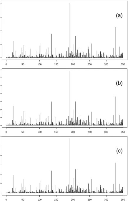
(2010), the read counts in each nucleotide in the same gene are highly heterogeneous, and highly correlated across tissues, which can be seen in Figure 2.1.

Figure 1 of Li et al. (2010) also suggests that the read counts in a nucleotide might have bias associated with its genomic position, which can be determined by the neighborhood nucleotides composition. Thus Li et al. (2010) considered associ-ating the read counts with neighborhood single nucleotide composition by additive models. In this paper, we develop a linear model relating the short read count at a nucleotide with its neighborhood overlapping dinucleotide compositions, through which the nucleotide interactions are naturally built in. We assume that the log transformed count of reads,yij = log(nij+ 1), depends onKu nucleotide pairs

imme-diately upstream andKd nucleotide pairs immediately downstream the read, denoted

as bij,−Ku, bij,−(Ku−1), . . . , bij,(Kd−1), bij,Kd, see Figure 2.2, through the following linear

model: yij =α+vi+ Kd X k=−Ku X h∈H βkhI(bijk =h) +ij, (2.1)

(19)

0 50 100 150 200 250 300 350 0 500 1000 1500 2000 Nucleotide Position Counts (a) 0 50 100 150 200 250 300 350 0 200 400 600 800 1000 1200 1400 Nucleotide Position Counts (b) 0 50 100 150 200 250 300 350 0 200 400 600 800 1000 1200 Nucleotide Position Counts (c) Nucleotide Position Count

Figure 2.1: Counts of reads along gene Apoe in different tissues of the Wold

(20)

Figure 2.2: An illustration of the neighborhood overlapping dinucleotide

composition A read is mapped to the genome starting at position 0. Upstream

positions are labeled as negative and downstream positions are labeled as positive. (AAwas used as baseline), αis the grand mean, vi is the main effect of genei, under

the constraintP

vi = 0,I(bij,k=h) equals 1 if thekth dinucleotide of the surrounding

sequence is h, and 0 otherwise, βkh is the coefficient of the effect of dinucleotide h

occurring in thekth position, and ij ∼N(0, σ2). LetK =Ku+Kd. The constant 1

is added to the original counts to account for positions with zero reads mapped. This linear model uses 15K+G parameters to model the sequence bias of read counts. It is worth noting that the trinucleotide composition may be considered in the model, but the large number of parameters, i.e, 63 parameters for each trinucleotide position, incurs a rapid surge of the computation costs for model-fitting.

2.2.2 Model-fitting and the Distance-weighted Penalized

Regression

In practice, the number of upstream nucleotides Ku and Kd in model 2.1 need to be

(21)

related dinucleotides are all included in the model. However, if we set Ku = 40 and

Kd = 40 (thus K = 80), we will have roughly 1200 dinucleotide coefficients βkh to

estimate. With such a huge number of coefficients, many of which are redundant, the calculations are unstable and error-prone. To alleviate the computational cost and to stabilize the algorithm, we use a penalized regression method to determine the number of nucleotides adaptively. Since the number of overlapping dinucleotides

K corresponds toK single nucleotides, our penalized regression directly searches for an optimal number of single nucleotides. Among penalized regression methods, the

L1 penalized likelihood procedure is very effective since the L1 penalty encourages

shrinkage of irrelevant predictors to be exactly zero. The standard L1 penalty uses

the same weights for different predictors. However, the predictors in our model are dinucleotides, and it is observed in Liet al.(2010) that the impact of the nucleotides on the modeling read counts becomes smaller as the nucleotides get further away from the mapped reads. We thus consider a distance-weighted L1 penalty (Zhu &

Liu (2009)) in our algorithm so different nucleotides are penalized according to their relative distance to the mapped reads.

Algorithm:

(1.) We first fit a single nucleotide model with distance-weighted penalty,

G X i=1 Li X j=1 ( yij −α−vi− Kd X k=−Ku X h∈H∗ β_kh∗ I(b∗_ijk=h) )2 +λ Kd X k=−Ku X h∈H∗ wk|βkh∗ |, (2.2)

where b∗_ijk is the nucleotide composition of the kth nucleotide away from the jth nucleotide in ith gene, λ is the tuning parameter and H∗ ₌ _{_{C, G, T}_} ₍_A _{was used}

as baseline). The weightwk >0 will be chosen to be proportional to a certain power

of distance between nucleotide j and the kth nucleotide in the surrounding sequence (Zou (2006), Zhu & Liu (2009)), i.e., wk = (|k|+ 1)γ. We use the LARS/Lasso

(22)

algorithm (a.k.a. the homotopy algorithm) to find the solutions for all values of λ. Even though the solution path for all values of λ can be effectively computed, it is still highly desirable that one solution is given for a carefully chosen value of λ. To choose a value of λ with a good balance of goodness-of-fit of the model and model parsimony, we minimize the Bayesian Information Criterion (BIC).

(2.) Based on the parameters of the penalized fit in step 1, we then select the new sequence endpoints K_u∗ = min{k :β_kh∗ 6= 0 ∀h∈ {C, G, T}}, and K_d∗ = max{k :

β_kh∗ 6= 0 ∀h∈ {C, G, T}}.

(3.) With the selected K_u∗ and K_d∗ and the dinucleotide expansion, we fit the model (2.1) using the least squares,

G X i=1 Li X j=1    yij−α−vi− K_d∗ X k=K∗ u X h∈H βkhI(bijk =h)    2 (2.3)

where H={CC, GG, T T, AC, CA, AG, GA, AT, T A, CG, GC, CT, T C, GT, T G}. The model with the updated surrounding sequence and fit using the dinucleotide expansion will then be used for estimation of gene expression levels.

2.3 Results and Discussion

2.3.1 Datasets

Our model was fitted to three genome-wide RNA-Seq datasets. These datasets will be referred to as Wold, Burge and Grimmond as in Liet al.(2010). The Wold data, which comes from Mortazavi et al. (2008) consists of 79, 76, and 70 million reads, which are of length 25, generated by Illumina’s Solexa. The 79, 76, and 70 million reads each correspond to a subdataset from brain tissue, liver tissue, and skeletal muscle tissue, respectively. Like Li et al. (2010), when fitting the data, we will use the top 100 genes according to RPKM. So for the brain, liver and muscle Wold datasets, we

(23)

are considering 146828, 171776 and 143570 nucleotides for each datasets’ 100 genes, respectively. The Burge data, which comes from Wanget al. (2008) consists of three subdatasets which will be referred to as G1, G2 and G3. G1 consists of adipose, brain and breast tissue. G2 consists of colon, heart and liver tissue. G3 consists of lymph node, skeletal muscle and testes tissue. Each has reads ranging from 61 to 77 million. The datasets G1, G2, and G3 each consider 157614, 125056 and 103394 nucleotides respectively. The Burge data was also generated from Illumina’s Solexa with reads of length 32. Lasty, the Grimmond data, of Cloonan et al. (2008) was generated from ABI’s SOLiD with an original read length of 35. (Some are truncated into 30 or 25 nucleotides to ensure high quality.) The data consists of two subdatasets, each consisting of 16 million reads from each of two cell lines, which will be referred to as EB (embryoid bodies) and ES (undifferentiated mouse embryonic stem cells). The EB subdataset’s top 100 genes considers 51751 nucleotides and the ES subdataset uses 64966 nucleotides. Reads were uniquely mapped using Seqmap (Jiang & Wong (2008)) allowing for two mismatches.

We use the read counts data for the top 100 genes as prepared by Liet al. (2010).

2.3.2 Tuning the Algorithm

Our algorithm requires several tuning parameters. In this section, we present some results of various choices we attempted for the parameters. As an assessment of goodness-of-fit, we calculated the Bayesian Information Criterion (BIC),

BIC =−2loglike + (15K +G) log

G X i=1 Li ! (2.4) where the log likelihood of the fitted model is,

loglike = G X i=1 Li X j=1 ( 1 2log 1 2πσˆ2 − (log(nij)−log(\nij))2 2ˆσ2 ) (2.5)

(24)

where log(\nij) is the fitted value of the model. ˆσ2 is the estimated σ2 using the

residual sum of squares.

Determining Weights for Penalized Least Squares

In the penalized regression, γ, the power of the weights, wk = (|k|+ 1)γ needs to

be determined. By fixing γ = 1,2, . . . ,10 one-at-a-time, we calculated BIC based on the resulting surrounding sequence, which is presented in Table 2.1. By inspecting Table 2.1, we can find the γ which results in the best BIC. For simplicity, we opt to use the cubic weight (γ = 3) as our final choice when determining a surrounding sequence as it frequently preforms very well.

γ 1 2 3 4 5 6 7 8 9 10 Wold Brain 2.38 2.38 2.38 2.38 2.41 2.38 2.40 2.58 2.66 2.86 Liver 2.56 2.56 2.55 2.55 2.57 2.55 2.58 2.74 2.80 3.00 Muscle 2.75 2.74 2.74 2.74 2.76 2.74 2.75 2.87 2.93 3.09 Burge G1 2.82 2.82 2.82 2.82 2.83 2.82 2.86 2.94 2.98 3.08 G2 3.06 3.06 3.04 3.04 3.06 3.04 3.06 3.14 3.18 3.28 G3 2.96 2.95 2.94 2.94 2.96 2.93 2.97 3.06 3.12 3.22 Grimmond EB 3.51 3.51 3.51 3.51 3.56 3.51 3.54 3.59 3.64 3.76 ES 3.31 3.25 3.26 3.25 3.28 3.26 3.30 3.35 3.40 3.49 Table 2.1: Bayesian Information Criterion (BIC) for linear model with

var-ious penalty weights, γ. BICs are scaled with respect to the sample size of the

(25)

Determining Surrounding Sequence

In our algorithm, the distance-weighted penalized regression results in a sparse set of parameters βkh. Since each nucleotide position has three associated βkh, we need to

translate the sparse set of parametersβkh into a sparse set of surrounding nucleotides.

In the second step of our algorithm, we select theKu as the upmostkwith allβkh 6= 0

for h∈ {C, G, T}, and Kd as the downmost k with allβkh 6= 0 for h∈ {C, G, T}. To

examine the effectiveness of this strategy, we compare it with an alternative strategy which selects Ku as the upmost k with at least one of βkh 6= 0 for h ∈ {C, G, T},

and Kd as the downmost k with at least one of βkh 6= 0 for h ∈ {C, G, T}. This

alternative strategy results in a larger Ku and Kd, however after refitting with the

dinucleotide expansion, the goodness-of-fit does not improve enough to justify the increased number of parameters. This suggests that the strategy used in step 2 is appropriate.

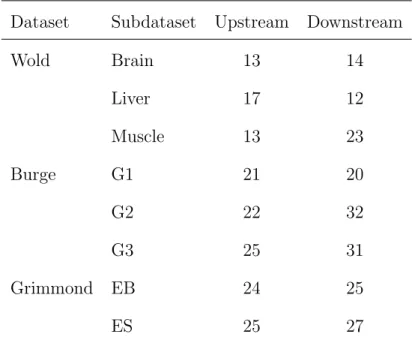
Table 2.2 presents the sequence lengths determined by our algorithm. Dataset Subdataset Upstream Downstream

Wold Brain 13 14 Liver 17 12 Muscle 13 23 Burge G1 21 20 G2 22 32 G3 25 31 Grimmond EB 24 25 ES 25 27

Table 2.2: The resulting surrounding sequence lengths upstream and down-stream of the reads.

(26)

This data-driven method of selecting a surrounding sequence gives different results from that in Li et al. (2010). We find shorter surrounding sequences are needed for the Wold datasets, but larger surrounding sequences for the Burge and Grimmond data.

Dinucleotide composition

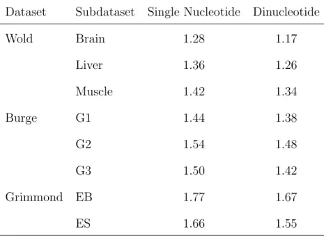
We also compare the linear model using neighborhood single nucleotide composition with the linear model using our neighborhood overlapping dinucleotide compositions. Table 2.3 presents the (negative) log likelihoods for the two models. We can see the (negative) log likelihood of the linear model with dinucleotide composition improves upon that with single nucleotide composition. This improvement can also be seen through an increase in R2. For example in the Wold Brain data, R2 is increased by 25%.

Dataset Subdataset Single Nucleotide Dinucleotide

Wold Brain 1.28 1.17 Liver 1.36 1.26 Muscle 1.42 1.34 Burge G1 1.44 1.38 G2 1.54 1.48 G3 1.50 1.42 Grimmond EB 1.77 1.67 ES 1.66 1.55

Table 2.3: Negative log-likelihoods for linear models with single nucleotide

expansion and the fit with the dinucleotide expansion. Both fit with

(27)

2.3.3 Comparison of Linear Models with the existing

Models

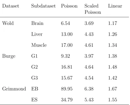
Dataset Subdataset Poisson Scaled Poisson Linear Wold Brain 6.54 3.69 1.17 Liver 13.00 4.43 1.26 Muscle 17.00 4.61 1.34 Burge G1 9.32 3.97 1.38 G2 16.81 4.64 1.48 G3 15.67 4.54 1.42 Grimmond EB 89.95 6.38 1.67 ES 34.79 5.43 1.55

Table 2.4: Negative log-likelihoods for Poisson and linear models. Likelihoods are scaled with respect to the sample size of the dataset. The Poisson models are fit with a surrounding sequence of 40. The surrounding sequences used for the linear model are the surrounding sequences found in Table 2.2.

We now compare our linear model with the Poisson and MART models in Liet al. (2010). As a direct comparison of goodness-of-fit, we consider the log-likelihoods of our linear model and the Poisson model (The MART model is an algorithmic method, thus the log likelihood cannot be calculated). Since the read counts are clearly over-dispersed, we also fit a scaled (over-dispersed) Poisson model as a fair comparison.

For the Poisson model, the log-likelihood is

loglike = G X i=1 Li X j=1 nij σ log( 1 σ ˆ nij σ )− ˆ nij σ −log ˆ nij! σ (2.6) where ˆnij is the fitted value of the model. For the scaled Poisson model σ is the

(28)

dispersion parameter estimated by a quasi-likelihood method (Wedderburn (1974)). For the unscaled Poisson model,σ is taken to be 1.

The resulting likelihood of the models for each dataset were summarized in Ta-ble 2.4. Even after adjusting for the dispersion, we see that the linear model outper-forms the scaled Poisson model in terms of log-likelihoods.

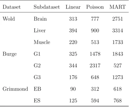
In addition to goodness-of-fit, the computational costs of our linear and existing models are also compared. Table 2.5 summarize the total runtime for each method.

Dataset Subdataset Linear Poisson MART

Wold Brain 313 777 2751 Liver 394 900 3314 Muscle 220 513 1733 Burge G1 325 1478 1843 G2 344 2317 527 G3 176 648 1273 Grimmond EB 90 312 618 ES 125 594 768

Table 2.5: Runtime for the Linear, Poisson and MART Models. CPU time (in seconds) for fitting the models obtained on a PC with an Intel Xeon E5540 processor and 24 Gbytes of RAM running openSUSE 11.4 and R 2.12.1. When fitting the linear model, the time used to determined the surrounding sequence is included.

When recording the runtime of the linear model, we include the time to deter-mine the surrounding sequence and the time to refit the model with the dinucleotide expansion. For the MART model, we use a predetermined surrounding sequence and use the default parameters for fitting as suggested by Liet al.(2010). From Table 2.5, we can clearly see that there is a substantial runtime difference between the Poisson and the linear models. This observation is most notable when fitting with the

(29)

dinu-0 50 100 150 200 250 0 1000 2000 3000 4000 Nucleotide Position Counts

(a)

0 50 100 150 200 250 0 1000 2000 3000 4000 Nucleotide Position Counts

(b)

0 50 100 150 200 250 0 1000 2000 3000 4000 Nucleotide Position Counts

(c)

Nucleotide Position Count

Figure 2.3: Predicted counts for gene Tnnc2. (a) True read counts for the Tnnc2 gene of the Wold muscle data. (b) Predicted counts for the linear model for the Tnnc2 gene. (c) Predicted counts for the Poisson model for the Tnnc2 gene.

(30)

cleotide expansion. As an example, for the wold brain Dataset the linear model (with sequence selection) runs roughly three times faster than the Poisson model, which uses an iterative re-weighted least squares algorithm.

2.3.4 Estimating Gene Expression Levels

Using our linear model, we have two methods to estimate gene expression levels. First, to estimate the gene expression for genei, we can use ˆα+ ˆvi from the estimated

model. As an alternative, we can also estimate the gene expression by bias-removed read counts Li X j=1 nij/Wi where Wi = Li X j=1 exp αˆ+ K X k=1 X h∈H ˆ βkhI(bijk =h) ! (2.7)

which is the sum of the sequence bias across all the nucleotide positions of gene i. Because there is no gold standard to validate the gene expression estimates, we opt to correlate our estimates with the estimates using the MART model in Li et al. (2010). We find that both methods are highly correlated with the results in Li et al. (2010) using the non-linear MART model with the sum of sequencing preferences. Our second method, using the sequence bias, does slightly better than the first method based on the estimated ˆα+ ˆvi. Table 2.6 shows the Spearman rank correlation between

the linear model and the MART model for each dataset using the sequence bias for gene expression estimation. Figure 2.4 compares the gene expression estimates of the MART method and the linear model.

Our work suggests that we can use the estimates from the linear model in place of the MART model. Since their results are very similar, the linear model may be a better choice due to its significantly lower computation time and easily interpretable parameters.

(31)

Wold Correlation ● ● ● ● ● ● ● ● ● ● ●●● ● ●● ● ● ● ●●● ● ●● ● ● ● ●● ● ●● ● ● ● ● ● ● ●● ●● ● ● ● ● ● ● ●● ●● ●● ● ● ●●● ●●● ● ● ● ●●● ●● ● ●●● ● ● ● ● ●● ●●●●●●●●●●●● ● ● ●●● ●● 0 1 2 3 1 2 3 4 5 6 LM Predicted MAR T Predicted Burge Correlation ● ● ●● ● ● ● ● ●● ● ● ● ● ● ● ● ● ● ● ● ● ● ● ● ● ● ● ● ● ● ● ● ● ● ● ● ● ● ●● ● ● ● ●● ● ●● ● ● ● ●● ● ● ● ● ● ● ● ●●● ● ● ● ● ● ● ● ● ● ● ● ● ● ● ● ● ● ● ● ● ● ●●●●● ● ●● ● ● ●● ● ● ● −0.5 0.0 0.5 1.0 1.5 2.0 2.5 2 3 4 5 6 LM Predicted MAR T Predicted Grimmond Correlation ● ● ● ● ● ● ● ● ● ● ● ● ● ● ● ● ● ● ● ● ● ● ● ● ● ● ● ● ● ● ● ● ● ● ● ● ● ● ● ● ● ● ● ● ● ● ● ● ● ● ●● ● ● ● ● ● ● ● ● ● ● ● ● ● ● ● ● ● ● ● ● ● ● ● ● ● ● ● ● ● ● ● ● ● ● ● ● ● ● ● ● ● ● ● ● ● ● ● ● −1 0 1 2 4 5 6 7 8 LM Predicted MAR T Predicted

Figure 2.4: Gene expression estimates of the MART and linear model. Es-timates of the expression are plotted for the linear and MART models fit on each subdataset of the Wold, Burge and Grimmond data. Subdatasets are differentiated by color and point shape. Plotted on a log scale.

(32)

Dataset Subdataset Correlation Wold Brain 99.2 Liver 99.4 Muscle 99.3 Burge G1 96.8 G2 95.6 G3 97.2 Grimmond EB 97.4 ES 98.0

Table 2.6: Spearman rank correlations between MART and linear model gene expression estimates.

2.4 Conclusion

We propose a linear model for the sequence bias in RNA-seq read counts data using the neighborhood overlapping dinucleotides. We develop a penalized least squares algorithm for model-fitting. Fitting the linear model using a penalized least squares approach, we use weights to penalize parameters which are further away from the read in the surrounding sequence. We then use a data-driven method to determine an appropriate number of dinucleotides in the neighborhood sequence. Finding the sparse set of surrounding sequence which captures as much variation of read counts as possible results in a great savings in computational cost, especially compared with a computationally intense method such as MART. We also find that the gene expression estimates from our model are highly correlated with the estimates from the non-linear model MART.

After publication of the work in this chapter, we were made aware of some addi-tional work in correcting bias in RNA-seq. In particular, Zhenget al.(2011) directly

(33)

corrects the gene expression estimates through nonparametric regression on all po-tential bias factors. Zheng et al.(2011) focuses on gene level bias whereas our paper focuses on base level (nucleotide) bias. Roberts et al. (2011b) develops a Markov model with 744 parameters to model both gene level and base level biases. Hu et al. (2012) develops a Poisson mixed effect model to model the base level bias one-gene-at-a-time. The computation of the latter two methods is expensive. On the other hand, the fragment bias considered in those papers may be integrated into our method to further improve the accuracy of transcript quantification.

(34)

Chapter 3 RNA-Seq Gene Expression

Quantification Using Transcript

Reads Variation

RNA-Seq, the current successor to DNA microarray technology, has become a popular tool for transcriptome analysis (Mortazavi et al. (2008), Nagalakshmi et al. (2008), Wilhelm et al. (2008)). By producing millions of short reads (sequences of A, C, T and G represent nucleotides) it offers detailed insight into the transcriptome. Af-ter mapping the reads to a reference genome or transcripts, RNA-Seq data provides quantification information for the entire genome with nucleotide level detail. A large amount of research has focused on transcript quantification, in particular, gene ex-pression calculation, using these short read counts. Mortazaviet al.(2008) develop a simple enumeration method, in which the expression level of a transcript is quantified as reads per kilobase of the transcript per million mapped reads to the transcriptome (RPKM). A variant, FPKM is developed in Trapnell et al. (2010) which is used for paired-end analysis. These analysis methods assume, explicitly or implicitly, a naive constant-rate Poisson model, Pois(λ), for short read counts and attempt to estimate the mean, λ, using the mean read count.

Some work has shown that short-read counts have significant biases, including sequence bias, where read counts are affected by the nucleotide composition of a sur-rounding region, see Dohmet al.(2008), thus reducing the effectiveness of some simple quantification methods such as RPKM. Thus, more elaborate statistical models that can effectively remove the sequence bias of the short-read counts are highly desirable to make transcript quantification more accurate. Liet al. (2010), Srivastava & Chen (2010) and Bullard et al. (2010) developed Poisson regression models with variable

(35)

rates for modeling the short-read counts. The previous chapter develops a method using a penalized linear regression using the surround dinucleotide composition of reads.

One issue with the Poisson models that has been observed is the presence of a much greater variance than mean. POME, “Poisson mixed-effects model,” is another recent model-based method developed by Huet al.(2012) which incorporates spatial dependence in an attempt to model this phenomena and has been shown to perform well. Other methods include Zheng et al. (2011) which uses GC content and dinu-cleotide composition to correct gene level bias and Robertset al. (2011b) which uses a complex Markov model to model both gene level and base level biases. While these statistical models do succeed in modeling and removing some bias that exist in the simple enumeration methods, this usually comes at the cost of significant computing time and power.

Both the simple enumeration estimators, such as RPKM, and the statistical meth-ods correcting for bias, use estimators based on the mean of the read counts. As an alternative, we propose estimators based on a mixture of the mean and variance. This is motivated by the property of the Poisson distribution that the mean and variance are equal, which makes the read count variance a natural estimator forλ. Estimators based on variation seem well suited as an estimator of expression levels. They place a much higher emphasis on the few very large read counts that occur.

Similar to methods such as RPKM, these estimators based on the read variation are simple enumeration methods which require very little computation. We demon-strate their accuracy and speed using multiple gold standard datasets for comparison with other methods.

(36)

Figure 3.1: Read counts for the Fth1 gene in skeletal muscle tissue

(Mor-tazavi et al. (2008))

3.1 Methods

After reads are mapped to the genome they are summarized as read counts, meaning at each position on the genome there will be an associated read count which quantifies the number of reads mapped to that position. This is done in one of two ways. Read counts can be defined as the number of reads which cover a position on the genome, or instead we will define a read count to be the number of reads that start from a particular position on the genome. Consider a short example gene of length ten with sequence ACTGTGGCTA. If we have 10 ACTGT reads, 12 CTGTG reads and 8 TGTGG reads, the resulting read counts for our example gene would be 10, 12, 8 and so on.

Letnij denote the counts of reads that are mapped to the genome starting at the

jth nucleotide of theith gene (or transcript), wherei= 1,2, . . . , G, j = 1, . . . , Li. We

then consider a number of estimators.

First, we establish definitions of RPKM. Technically, RPKM is defined as Reads Per Kilobase of transcript per Million mapped. Thus the RPKM of gene i is defined

(37)

as RP KMi = PLi j=1nij Li 1000 PG i=1 PLi j=1nij 1000000 ! (3.1)

For ease of presentation we will refer to two simplified variants of RPKM.

oRP KMi = ¯ni = PLi j=1nij Li (3.2) eRP KMi = PLi j=1nij PLi j=1I[nij 6= 0] (3.3) oRPKM is simply the sample mean of the number of reads mapped to a gene or transcript. For simplicity we do not consider the the scaling based on million mapped reads and length of transcript. (For the comparison methods used later, the total number of mapped reads is not relevant, however when analyzing multiple real datasets it is important for normalization.) eRPKM is similar, however only considers positions on the gene where reads were mapped.

We then propose a general estimator based on a mixture of the first and second moments, T RVi = v u u t 1 Li Li X j=1 n2_ij + (ρ2 ₋_1)¯_n2 i (3.4)

which we call the Transcript Reads Variation, or TRV. ρ is used as a tuning parameter which can be adjusted to place greater emphasis on the first or second moment. With ρ = 0 this is the sample standard deviation of the reads. Likewise,

ρ = 1 gives the square root of the sample second moment. (In other words, it is simply the the square root of the sum of the read counts divided by the length of the transcript.) By allowing added emphasis on the squared read counts, positions with

(38)

extremely large read counts contribute substantially more to the expression level. We now want to provide a rationalization for the proposal of these estimates. A common assumption is to model the read counts with a Poisson distribution. Follow-ing this convention, we consider the true read counts to be Poisson(λi), where λi is

the population mean read counts. Similarly consider the observed read counts to be Poisson(λO_i ) and the missing read counts Poisson(λM_i ). These missing reads can arise from the reads that are not mapped based on the criteria selected by the researcher or limitations of the technology. For example, using the common mapping tool Bowtie (Langmead et al. (2009)), a read may map with too many mismatches and is thus discarded.

Assuming then that the true reads are the sum of the observed and the missing reads, we wish to estimate

λi =λOi +λ M

i (3.5)

Since the Poisson distribution has the property that its mean is equal to its vari-ance, we the use

ˆ λO_i = 1 Li Li X j=1 (nij −n¯i)2 (3.6) to estimate λO i .

We wish to also use a variance estimator to estimate λM

i . To do so we use ρ2n¯2i,

so

ˆ

λM_i =ρ2n¯2_i (3.7)

(39)

ˆ λi = 1 Li Li X j=1 n2_ij + (ρ2−1)¯n2_i (3.8) which with a square root is our TRV estimator.

Through our results from real data examples, we note that ρ= 1 is a good choice for the TRV. Withρ= 1, which is only a function of the second moment, we refer to the estimator as TRV2, thus

T RV2i = v u u t 1 Li Li X j=1 n2 ij (3.9)

3.2 Results

3.2.1 Datasets

Helicos Prostate Cancer Data

The first dataset contains 12 RNA samples from prostate cancer related cells which were generated by the Chinnaiyan lab at the University of Michigan. (Sam et al. (2011)) The data can be obtained using accession numbers SRA028835 from the NCBI Sequence Read Archive. The samples were sequenced using the Helicos plat-form which uses single-molecule sequencing technology, meaning reverse transcription is avoided and the RNA is sequenced directly. By not using reverse transcription, PCR amplification avoided, thus making it is a more direct measurement. Our method will be applied to the reads generated from these samples using the Illumina Genome An-alyzer and the estimates using the Helicos platform will be used as the gold standard for comparison. The Illumina reads were aligned using Bowtie with two mismatches allowed and the best alignment reported.

(40)

MAQC Brain and UHR Data

The second dataset, from the MicroArray Quality Control project (MAQC Consor-tium (2006)), contains two samples sequenced using Illumina technology. The Univer-sal Human Reference (UHR) and Human Brain Reference (Brain) samples both have seven lanes of sequencing available. Both can be obtained using accession numbers SRA010153 and SRA008403 from the NCBI Sequence Read Archive. For each sample, the MAQC project generated expression levels for over 1000 genes using quantitative real-time reverse transcription polymerase chain reaction (qRT-PCR) using TaqMan Gene Expression Assay. Our method will be applied to the reads generated from these samples using the Illumina Genome Analyzer and the estimates using TaqMan Gene Expression Assay will be used as the gold standard for comparison. Illumina reads were aligned using Bowtie with two mismatches allowed and only unique alignments reported.

3.2.2 Comparison to Gold Standards

We compared the various TRV estimators to both RPKM estimators as well as a statistical method, POME, which has shown good performance. POME, or “Poisson mixed-effects model,” is a recent model-based method developed by Hu et al., which incorporates spatial dependence. The read counts for geneiat positionj are modeled as

nij|θi, Uij, Vij ∼P oisson(Liθiexp[Uij +Vij])

where the fixed-effectθiis the expression level of geneiandUij andVij are random

effects used to account for the spatial dependence. The model is fit using Markov chain Monte Carlo methods, which require substantial computing time.

(41)

Sample ρ= 0 ρ= 0.5 ρ= 1 LnCaP0 0.693 0.694 0.698 LNCaP24 0.690 0.691 0.693 LnCaP48 0.642 0.642 0.643 VCaP0 0.649 0.650 0.651 VcaP24 0.666 0.667 0.668 VcaP48 0.708 0.708 0.709 aT34 0.573 0.572 0.572 aT34N 0.511 0.511 0.511 DU145F 0.628 0.628 0.629 DU145F2 0.630 0.630 0.631 VCaP 0.527 0.526 0.525 RWPE 0.603 0.604 0.605

Table 3.1: Spearman correlation of the gold standard expressions (estimates derived from the Helicos technology) and various estimates applied to the Illumina RNA-Seq data for each of the twelve samples in the prostate cancer dataset. Bold correlations indicate the highest correlation for each sample. ρ= 1 will be known as TRV2.

using the Helicos technology in the prostate cancer dataset. Table 3.1 compares the TRV estimators with various tuning parameters to the gold standard Helicos data. Table 3.2 shows the Spearman rank correlation of various estimates and the estimates derived from Helicos. We see that in most samples, the TRV2 estimator achieves the highest correlation with the gold standard.

Correlations were also calculated for some estimates and the gold standard esti-mates in the brain and UHR MAQC datasets obtained using qRT-PCR. Table 3.3 shows the Spearman rank correlation of the various estimates compared with the qRT-PCR estimates from the MAQC project. Also Table 3.4 shows the correlations

(42)

Sample eRPKM POME oRPKM TRV2 LnCaP0 0.624 0.688 0.691 0.698 LNCaP24 0.618 0.672 0.679 0.693 LnCaP48 0.600 0.640 0.619 0.643 VCaP0 0.580 0.604 0.650 0.651 VcaP24 0.598 0.623 0.666 0.668 VcaP48 0.622 0.656 0.697 0.709 aT34 0.578 0.595 0.527 0.572 aT34N 0.428 0.394 0.497 0.511 DU145F 0.594 0.635 0.584 0.629 DU145F2 0.593 0.626 0.587 0.631 VCaP 0.520 0.517 0.497 0.525 RWPE 0.560 0.601 0.597 0.605

Table 3.2: Spearman correlation of the gold standard expressions (estimates derived from the Helicos technology) and TRV estimators with various tuning parameters applied to the Illumina RNA-Seq data for each of the twelve samples in the prostate cancer dataset. Bold correlations indicate the highest correlation for each sample. TRV2 is TRV with ρ= 1.