Trajectory-based differential expression analysis for single-cell sequencing data

(1)

Trajectory-based differential expression analysis

for single-cell sequencing data

Koen Van den Berge

1,2,3

, Hector Roux de Bézieux

4,5

, Kelly Street

6,7

, Wouter Saelens

1,8

,

Robrecht Cannoodt

8,9,10

, Yvan Saeys

1,8

, Sandrine Dudoit

3,4,5,11

✉

& Lieven Clement

1,2,11

✉

Trajectory inference has radically enhanced single-cell RNA-seq research by enabling the study of dynamic changes in gene expression. Downstream of trajectory inference, it is vital to discover genes that are (i) associated with the lineages in the trajectory, or (ii) differen-tially expressed between lineages, to illuminate the underlying biological processes. Current data analysis procedures, however, either fail to exploit the continuous resolution provided by trajectory inference, or fail to pinpoint the exact types of differential expression. We intro-duce tradeSeq, a powerful generalized additive model framework based on the negative binomial distribution that allowsﬂexible inference of both within-lineage and between-lineage differential expression. By incorporating observation-level weights, the model additionally allows to account for zero inﬂation. We evaluate the method on simulated datasets and on real datasets from droplet-based and full-length protocols, and show that it yields biological insights through a clear interpretation of the data.

https://doi.org/10.1038/s41467-020-14766-3 OPEN

1_{Department of Applied Mathematics, Computer Science and Statistics, Ghent University, Ghent, Belgium.}2_{Bioinformatics Institute Ghent, Ghent University,} Ghent, Belgium.3Department of Statistics, University of California, Berkeley, CA, USA.4Division of Biostatistics, School of Public Health, University of California, Berkeley, CA, USA.5Center for Computational Biology, University of California, Berkeley, CA, USA.6Department of Data Sciences, Dana-Farber Cancer Institute, Boston, MA, USA.7_{Department of Biostatistics, Harvard T.H. Chan School of Public Health, Boston, MA, USA.}8_{Data mining and Modelling} for Biomedicine, VIB Center for In_ﬂammation Research, Ghent, Belgium.9_{Center for Medical Genetics, Ghent University Hospital, Ghent, Belgium.} 10_{Department of Biomolecular Medicine, Ghent University, Ghent, Belgium.}11_{These authors contributed equally: Sandrine Dudoit, Lieven Clement.}

✉email:[email protected];[email protected]

123456789

(2)

S

ingle-cell transcriptome sequencing (scRNA-seq) has

revo-lutionized modern biology by allowing researchers to proﬁle

transcript abundance at the resolution of an individual cell. This has opened new avenues of research to study cellular pathways during the cell cycle, cell-type differentiation, or cellular activation. Indeed, scRNA-seq can provide a snapshot of the transcriptome of thousands of single cells in a cell population, which are each at distinct points of the dynamic process under study. This wealth of transcriptional information, however, pre-sents many data analysis challenges. Until recently, statistical and computational efforts have focused mostly on trajectory inference

(TI) methods, which aim toﬁrst allocate cells to lineages and then

order them based on pseudotimes within these lineages. A wide range of TI methods have been proposed; 45 of which are

extensively benchmarked in Saelens et al.1. Note that we use the

term ‘trajectory’ to refer to the collection of ‘lineages’ for the

process under study.

Most TI methods share a common workﬂow: dimensionality

reduction followed by inference of lineages and pseudotimes in

the reduced dimensional space2_{. In that reduced dimensional}

space, a cell’s pseudotime for a given lineage is the distance, along

the lineage, between the cell and the origin of the lineage. As such, while pseudotime can be interpreted as an increasing function of true chronological time, there is no guarantee that the two follow a linear relationship. Recent developments have allowed the

inference of complex trajectories3–5_{. These advances enable}

researchers to study dynamic biological processes, such as com-plex differentiation patterns from a progenitor population to

multiple differentiated cellular states6,7_{, and have the promise to}

provide transcriptome-wide insights into these processes. Unfortunately, statistical inference methods are lacking to identify genes associated with lineage differentiation and to

unravel how their corresponding transcriptional proﬁles are

driving the dynamic processes under study. Indeed, differential expression (DE) analysis of individual genes along lineages is often performed on discrete groups of cells in the developmental pathway, e.g., by comparing clusters of cells along the trajectory or clusters of differentiated cell types. Such discrete DE approa-ches do not exploit the continuous expression resolution that can be obtained from the pseudotemporal ordering of cells along lineages provided by TI methods. Moreover, comparing cell clusters within or between lineages can obscure interpretation: it is often unclear which clusters should be compared, how to properly combine the results of several pairwise cluster compar-isons, or how to account for the fact that not all of these com-parisons are independent of each other.

A number of methods have been developed for the analysis of bulk RNA-seq time-series data, which can exploit the temporal

resolution of samples assayed at different times8–10_{. However, in}

scRNA-seq, the relationship between gene expression and pseu-dotime is more complex. In addition, the pseupseu-dotimes are con-tinuous, and cells are never at the exact same pseudotime value. A few methods have been published with the aim of improving trajectory-based differential expression analysis by modeling gene expression as a smooth function of pseudotime along lineages.

Monocle11 _{tests whether gene expression is associated with}

pseudotime by ﬁtting additive models of gene expression as a

function of pseudotime. However, the method can only handle a

single lineage. A similar approach has been adopted by TSCAN12_.

GPfates4relies on a mixture of overlapping Gaussian processes13,

where each component of the mixture model represents a dif-ferent lineage. For each gene, the method tests whether a model

with a bifurcation signiﬁcantly increases the likelihood of the data

as compared with a model without a bifurcation, essentially testing whether gene expression is differentially associated with

the two lineages. Similarly, the BEAM approach in Monocle 25

allows users to test whether differences in gene expression are associated with particular branching events on the trajectory. These trajectory-based methods improve upon discrete cluster-based approaches by (1) exploiting the continuous expression resolution along the trajectory and (2) comparing lineages using a

single test based on entire gene expression proﬁles. However,

both GPfates and Monocle 2 lack interpretability, as they cannot

pinpoint the regions of the gene expression proﬁles that are

responsible for the differences in expression between lineages. Moreover, the GPfates model is restricted to trajectories con-sisting of just one bifurcation, essentially precluding its applica-tion to biological systems with more than two lineages (i.e., a multifurcation or more than one bifurcation). BEAM is restricted to the few dimensionality reduction methods that are imple-mented in the Monocle 2 software, namely, independent

com-ponent analysis (ICA) and DDRTree5_{. Hence, novel methods to}

infer differences in gene expression patterns within or between transcriptional lineages with complex branching patterns are vital

to further advance theﬁeld.

In this paper, we introduce tradeSeq, a method and software

package for trajectory-based differential expression analysis for

sequencing data. tradeSeq provides aﬂexible framework that can

be used downstream of any dimensionality reduction and TI method. Unlike previously proposed approaches, tradeSeq pro-vides several tests that each identify a distinct type of differential expression pattern along a lineage or between lineages, leading to

clear interpretation of the results (Fig. 1). In practice, tradeSeq

infers smooth functions for the gene expression measures along pseudotime for each lineage using generalized additive models and tests biologically meaningful hypotheses based on parameters of these smoothers. By allowing cell-level weights for each indi-vidual count in the gene-by-cell expression matrix, tradeSeq can

handle zero inﬂation, which is essential for dealing with dropouts

in full-length scRNA-seq protocols14. As it is agnostic to the

dimensionality reduction and TI methodology, the approach scales from simple to complex trajectories with multiple bifur-cations: tradeSeq only requires the original expression count matrix of the individual cells, estimated pseudotimes, and a hard or soft assignment (weights) of the cells to the lineages to infer the

lineage-speciﬁc smoothers. We benchmark our method against

current state-of-the-art methods using simulated data sets (with cyclic, bifurcating, and multifurcating trajectories) and demon-strate its functionality and versatility on four real data sets. These

case studies highlight the enhanced interpretability of tradeSeq’s

results, which lead to improved understanding of the underlying biology.

Results

Statistical model and inference using tradeSeq. We model gene

expression measures as nonlinear functions of pseudotime using a generalized additive model (GAM). In the GAM, each lineage is

represented by a separate cubic smoothing spline, and theﬂ

ex-ibility of GAMs allows us to adjust for other covariates or

con-founders asﬁxed effects in the model. The read countsYgi, for a

given geneg∈{1,…,G} across cellsi∈{1,…,n} are modeled

using a negative binomial GAM (NB-GAM) with cell and

gene-speciﬁc meansμgiand gene-speciﬁc dispersion parametersϕg:

Y_giNBðμ_gi;ϕ_gÞ logðμ_giÞ ¼η_gi η_gi¼PL l¼1sglðTliÞZliþUiαgþlogðNiÞ: 8 > > < > > : ð1Þ

The gene-wise additive predictor ηgi consists of lineage-speciﬁc

smoothing splines sgl, that are functions of pseudotime Tli, for

(3)

l ∈{1, …, L}, i ∈{1, …, n}) assigns every cell to a particular

lineage based on user-supplied weights (e.g., from slingshot3 or

GPfates4_{, see details in Supplementary Methods). We let} _L

l ¼

fi:Z_li¼1g denote the set of cells assigned to lineage l. In

addition, we allow the inclusion of pknown cell-level covariates

(e.g., batch, age, or gender), represented by an n×p matrixU,

with ith row Ui corresponding to the ith cell, and regression

parameters αg of dimension p× 1. Differences in sequencing

depth or capture efﬁciency between cells are accounted for by

cell-speciﬁc offsetsNi.

The smoothing splinesgl, for a given genegand lineagel, can

be represented as a linear combination ofKcubic basis functions,

sglðtÞ ¼

XK k¼1

bkðtÞβglk; ð2Þ

where the cubic basis functionsbk(t) are enforced to be the same

for all genes and lineages.

Since a separate smoothing spline is estimated for every lineage in the trajectory, we can assess DE within or between lineages by

comparing the parameters βglk of these smoothing splines, see

“Methods”for details. In tradeSeq, we have implemented Wald

tests to assess DE and provide a range of different testing

procedures that allow biologists to interpret complex trajectories

in dynamic biological systems (see Fig.2).

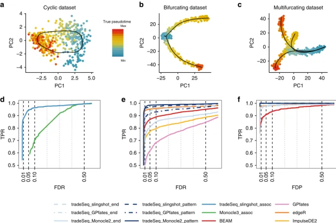
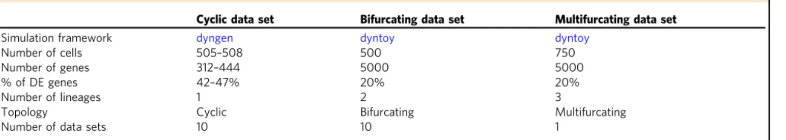
Simulation study. To benchmark relevant differential expression

methods, we generated multiple data sets, spanning three distinct

trajectory topologies (Fig. 3a–c), using the independently

devel-oped dynverse toolbox1_(see_“_Methods_”_{). Note that the simulated}

data sets are relatively“clean”, as reﬂected by the high sensitivity

and speciﬁcity of most methods. In particular, cells are

approxi-mately uniformly distributed along each lineage and often balanced between lineages. The data sets are, however, still useful to provide a relative ranking of the methods.

We demonstrate the versatility of tradeSeq by using it

downstream of three trajectory inference methods, slingshot3_,

Monocle 25_{, and GPfates}4_{, which will be denoted by}

tradeSeq_-slingshot, tradeSeq_Monocle2, and tradeSeq_Gpfates,

respec-tively. However, we ﬁnd that GPfates fails to recover the

expected trajectory topology if run in an unsupervised way (Supplementary Fig. 3a). Feeding the true pseudotimes as input to GPfates may, however, result in meaningful trajectories (Supple-mentary Fig. 3b). We therefore adopt this approach in the simulation study, but note that this may provide an a priori

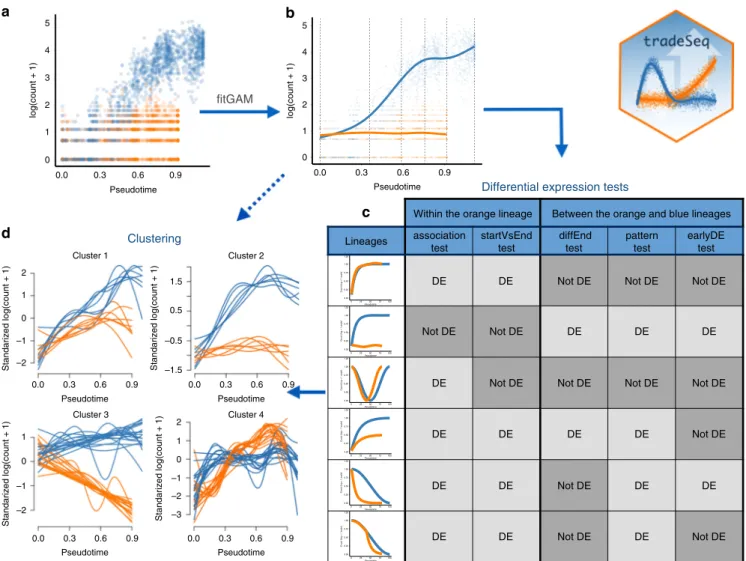
0 1 2 3 4 5 0 1 2 3 4 5 a b c d 0.0 0.3 0.6 0.9 Pseudotime 0.0 0.0 2 1.5 0.5 –0.5 –1.5 1 0 –1 –2 2 1 1 0 –1 –2 0 –1 –2 –3 0.3 0.3 0.6 0.6 0.9 0.9 Pseudotime fitGAM Pseudotime Cluster 1 Clustering

Standarized log(count + 1) Standarized log(count + 1)

Standarized log(count + 1) Standarized log(count + 1) Cluster 2 Cluster 4 Cluster 3 0.0 0.3 0.6 0.9 Pseudotime 0.0 0.3 0.6 0.9 Pseudotime 0.0 0.3 0.6 0.9 Pseudotime log(count + 1) log(count + 1) 0.00 0.25 0.50 0.75 1.00 1.25 0 25 50 75 100 Pseudotime

Count (log + 1 scale)

0.00 0.25 0.50 0.75 1.00 1.25 0 25 50 75 100 Pseudotime

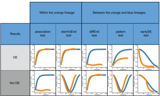
Differential expression tests

Within the orange lineage Between the orange and blue lineages

Lineages association test startVsEnd test diffEnd test pattern test earlyDE test

DE DE Not DE Not DE Not DE

Not DE Not DE DE DE DE

DE Not DE Not DE Not DE Not DE

DE DE DE DE Not DE

DE DE Not DE DE DE

DE DE Not DE DE Not DE

Fig. 1 Overview of tradeSeq functionality. aA scatterplot of expression measures vs. pseudotimes for a single gene, where each lineage is represented by a different color (top left).bA negative binomial generalized additive model (NB-GAM) is_fitted using the_fi_tGAMfunction. The locations of the knots for the splines are displayed with gray dashed vertical lines.cThe NB-GAM can then be used to perform a variety of tests of differential expression within or between lineages. In the table, we assume that theearlyDETestis used to assess differences in expression patterns early on in the lineage, e.g., with optionknots=c(1, 2), meaning that we test for differential patterns between thefirst and second dashed gray lines from panel (b).dInteresting genes canfinally be clustered to display the different patterns of expression.

(4)

competitive advantage to GPfates over other TI methods and that this would be impossible for real data sets.

Existing frameworks for differential expression analysis are not modular, in the sense that the DE method is tied to the TI method implemented in the same software package. Because of this, the comparison of DE methods is confounded with the quality of the upstream trajectory inference. We therefore also evaluate all trajectory-based DE methods by using the simulation ground truth as input for the DE analysis, which avoids such a confounding. GPfates was left out of this comparison, since we were not able to input the simulation ground truth to the method. Within-lineage DE: First, we look for genes whose expression is associated with pseudotime for data sets with a cyclic topology

(e.g., Fig. 3a). We compare the associationTest of a

tradeSeq_slingshot analysis to the Moran’s I test implemented in

Monocle 3. We apply tradeSeq using 5 knots, as determined using the AIC (Supplementary Fig. 4). We only consider Monocle 3 because it is the only method that provides a test of the association between gene expression and pseudotime within a single lineage. For each TI method, we use the default/ recommended dimensionality reduction method, which is PCA for slingshot and UMAP for Monocle 3.

Monocle 3, however, often fails to reconstruct the cyclic

topology and instead may ﬁt a disconnected or branching

trajectory (Supplementary Fig. 5). The Moran’s I test still has

reasonably high sensitivity, possibly because it relies on nearest neighbors in the reduced dimensional space and not on the inferred trajectory. tradeSeq downstream of slingshot provides superior performance to discover genes whose expression is

associated with pseudotime (Fig. 3d). We also compared both

methods using the same dimensionality reduction input, by having slingshot infer trajectories in the UMAP space that is used by Monocle 3. The performance of tradeSeq was generally similar for both dimensionality reduction methods, except for two out of ten data sets (Supplementary Fig. 6). In all data sets, tradeSeq had better performance than Monocle 3. Finally, we evaluate an

edgeR-based associationTest through ﬁtting the

NB-GAMs with edgeR instead of with mgcv (method edgeR_assoc,

see “Methods” for details), and note that its performance is

similar to the tradeSeq associationTest (Supplementary

Fig. 7). This could be expected because few basis functions were selected for this simulation setting. In applications that require a rich basis, however, the edgeR implementation will be prone to

overﬁtting.

Between-lineage DE: For the bifurcating data sets (e.g., Fig.3b),

we assess differential expression between lineages using the

diffEndTestand the patternTestfrom tradeSeq, down-stream of TI methods slingshot, Monocle 2, and GPfates. We apply tradeSeq with four knots, as determined using the AIC (Supplementary Fig. 8). We compare these tests with available approaches for trajectory-based differential expression analysis, namely, BEAM (implemented in Monocle 2), GPfates, and ImpulseDE2. Furthermore, we compare against the discrete DE method edgeR, where we supervise the test to assess DE between the clusters at the true endpoints of each lineage, as derived

throughk-means clustering in PCA space. For each TI method,

we use the default/recommended dimensionality reduction, which is PCA for slingshot, GPLVM for GPfates, and DDRTree for Monocle 2. For ImpulseDE2, we use the same input as for tradeSeq, i.e., derived by slingshot TI.

Monocle 2 and GPfates fail to detect the correct topology of the trajectory (i.e., a bifurcation) in, respectively, three and four out of the ten data sets (Supplementary Figs. 9 and 10). In addition, out of the remaining seven data sets, Monocle 2 misplaces the bifurcation in four of them, causing the two simulated lineages to be merged into the same lineage and creating another incorrect lineage (Supplementary Fig. 9). This strongly obscures the DE

testing results. slingshot, on the other hand, correctly identiﬁes

the topology and reconstructs the trajectory for all ten data sets.

Figure3e shows performance curves for the three data sets for

which all methods are able to recover the true topology of the

simulated trajectory. The tradeSeq patternTesthas superior

performance regardless of the TI method. Only edgeR achieves a similar performance. This is not surprising since the edgeR analysis is supervised to compare the true cell populations at the

endpoints of the lineages. Interestingly, tradeSeq’s

diffEndT-estbased on the slingshot trajectory performs comparably with

a supervised edgeR analysis. This is especially encouraging, since

Within the orange lineage

Results DE 1.25 1.00 0.75 0.50

0.25 0.00 1.25 1.00 0.75 0.50

0.25 0.00 0 25 50 Pseudotime 75 100 0 25 50 Pseudotime 75 100 0 25 50 Pseudotime 75 100 0 25 50 Pseudotime 75 100 0 25 50 Pseudotime 75 100 0 25 50 Pseudotime 75 100 0 25 50 Pseudotime 75 100 0 25 50 Pseudotime 75 100 0 25 50 Pseudotime 75 100 0 25 50 Pseudotime 75 100 1.25 1.00 0.75 0.50

0.25 0.00 Not DE association test startVsEnd test diffEnd test pattern test earlyDE test Between the orange and blue lineages

Fig. 2 Tests currently implemented in the tradeSeq package.Each column corresponds to a test. Tests are broken down into two categories, depending on whether they concern a within-lineage comparison, i.e., properties of the orange curve, or a between-lineage comparison, i.e., contrasting the blue and orange curves. For each test, we have two toy examples of gene expression patterns. The top one corresponds to a differentially expressed gene according to the test, while the bottom one does not.

(5)

thediffEndTestis a smoother-based analog of discrete DE.

For TI methods Monocle 2 and GPfates, diffEndTest

performs poorly, which is not surprising since the endpoints

are typically ill-deﬁned or artiﬁcially extended in the inferred

trajectories for these methods (Supplementary Figs. 9 and 10). In general, BEAM, ImpulseDE2, and GPfates are outperformed by the other methods. Across all methods, tradeSeq_slingshot has the best performance. Finally, we recapitulate that the

perfor-mance curves in Fig. 3e do not provide a complete view of

method performance, since seven out of ten data sets were not used because at least one method failed to recover the simulated trajectory. Supplementary Fig. 11 shows mean performance curves across all ten data sets for all methods, which clearly demonstrates the superiority of tradeSeq as a DE method and of slingshot as an upstream TI method. The performance and trajectories for all ten individual data sets are shown in Supplementary Fig. 12.

In order to avoid the comparison of DE methods being obscured by differences in the upstream dimensionality reduction and trajectory inference methods, we compared tradeSeq, BEAM,

and ImpulseDE2 on the simulation ground truth. We ﬁt the

tradeSeq NB-GAM once with three knots, for comparability with the BEAM approach that also uses three knots, and once with

four knots, which was found to be optimal according to the AIC

(Supplementary Fig. 8). The tradeSeq patternTest is

unaffected by the change in the number of knots and outperforms all other methods for differential expression analysis

(Supple-mentary Fig. 13). The performance of the tradeSeq

diffEndT-estis somewhat sensitive to the number of knots, but still better

than that of ImpulseDE2 and BEAM. Generally, ImpulseDE2 performs better than the BEAM approach.

For the multifurcating data set, we forego a comparison with GPfates, since it is restricted to discovering only a single

bifurcation (Supplementary Fig. 14). We ﬁt tradeSeq with three

knots, as determined using the AIC (Supplementary Fig. 15). The

patternTest from tradeSeq_slingshot and tradeSeq_Mono-cle2 have highest performance, closely followed by edgeR and the

diffEndTestfor these respective TI methods (Fig.3f). BEAM was found to have the lowest performance.

Taken together, these results suggest that tradeSeq is a

powerful and ﬂexible procedure for assessing DE along and

between lineages. Although tradeSeq is modular and can be used downstream of any TI method that provides pseudotime estimates, the choice of dimensionality reduction and TI method is crucial for the performance of the downstream analysis. The best performance was found for a tradeSeq_slingshot analysis, so

−4 −2 0 2 4 −2.5 0.0 2.5 5.0 PC1 PC2 Cyclic dataset a −40 −20 0 20 −25 0 25 PC1 PC2 Bifurcating dataset b −20 0 20 40 −20 0 20 40 PC1 PC2 Multifurcating dataset c 0.5 0.6 0.7 0.8 0.9 1.0 0.01 0.05 0.10 0.50 FDR TPR d 0.5 0.6 0.7 0.8 0.9 1.0 0.01 0.05 0.10 0.50 FDR TPR e 0.5 0.6 0.7 0.8 0.9 1.0 0.01 0.05 0.10 0.50 FDP TPR f tradeSeq_slingshot_end tradeSeq_GPfates_end tradeSeq_Monocle2_end tradeSeq_slingshot_pattern tradeSeq_GPfates_pattern tradeSeq_Monocle2_pattern tradeSeq_slingshot_assoc Monocle3_assoc BEAM GPfates edgeR ImpulseDE2 True pseudotime Max Min

Fig. 3 Simulation study results.PCA plots for the (a) cyclic, (b) bifurcating, and (c) multifurcating simulated trajectories. The plotting symbol for each cell is colored according to its true pseudotime; trajectories (in black) were inferred by princurve in (a) and slingshot in (b) and (c).d_–fScatterplot of the true positive rate (TPR) vs. the false discovery rate (FDR) or false discovery proportion (FDP) for various DE methods applied to the simulated data sets. Panel (d) displays the average performance curves of DE methods across seven out of ten cyclic data sets for which all DE methods worked (Monocle 3 errored on three data sets). TheassociationTestfrom tradeSeq has superior performance for discovering genes whose expression is associated with pseudotime, as compared with Monocle 3. When investigating differential expression between lineages of a trajectory, the_patternTestof tradeSeq consistently outperforms thediffEndTestacross all three TI methods, since it is capable of comparing expression across entire lineages. Panel (e) displays the average performance curves across the three bifurcating data sets where all TI methods recovered the correct topology. Here, all tradeSeq

patternTestwork_ﬂows, tradeSeq_slingshot_end, and edgeR have similar performance and all are superior to BEAM, ImpulseDE2, and GPfates. Note that the performance of tradeSeq_Monocle2_end deteriorates as compared with tradeSeq_slingshot_end; the curve for tradeSeq_GPfates_end is not visible in this panel due to its low performance. For the multifurcating data set of panel (f), tradeSeq_slingshot has the highest performance, closely followed by tradeSeq_Monocle2 and edgeR.

(6)

we will mainly focus on slingshot as TI method for the real data sets.

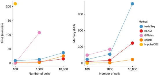
Computation time and memory-usage benchmark. To assess

time and memory requirements, scRNA-seq data sets with a bifurcating trajectory were simulated using the same framework

as in the simulation study; the results are shown in Fig. 4, and

more extensively described in Supplementary Note 1. Brieﬂy,

ImpulseDE2 is by far the slowest, taking over 3.5 h to run on a small data set of 100 cells. GPfates runs fast ( ~30 s) on the small data set, but scales poorly. BEAM, edgeR, and tradeSeq are quite fast and scale very well, even to large data sets, with BEAM scaling the best. In terms of memory requirements, all methods scale well to 10,000 cells.

Case studies. We analyze four case study data sets with tradeSeq:

a bulk RNA-seq time-course and scRNA-seq MARS-seq, Smart-Seq, and 10× data sets. While we discuss the MARS-seq and Smart-seq data sets in the main paper and their corresponding Supplementary Notes (see below), we only report the results for the bulk RNA-seq time-course and 10× data sets in Supple-mentary Notes 2 and 3, respectively.

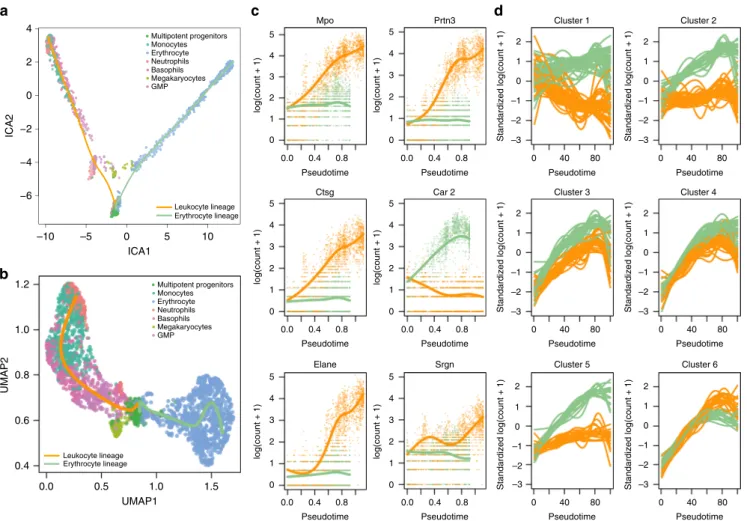
Mouse bone marrow data set. Paul et al.15study the evolution of

gene expression for myeloid progenitors in mouse bone marrow. They construct a reference compendium of marker genes that are indicative of development from myeloid multipotent progenitors to erythrocytes and several types of leukocytes.

In order to compare our approach with BEAM, we are restricted to the dimensionality reduction procedures

implemen-ted in Monocle 2. We thereforeﬁrst used ICA as dimensionality

reduction method (Fig.5a) in the“Discovering cell type markers”

paragraph, but observed that this approach does not fully preserve the underlying biology (Supplementary Note 4). In subsequent sections, we will therefore demonstrate the powerful interpretation of a tradeSeq_slingshot analysis based on UMAP

dimensionality reduction (Fig. 5b). This additionally illustrates

the ﬂexibility of tradeSeq (and slingshot) to be applied

down-stream of any dimensionality reduction method.

In this case study, we apply tradeSeq with six knots, as found to

be optimal by the AIC (Supplementary Fig. 22). Weﬁrst identify

marker genes for the progenitor and differentiated cell types in

the “Discovering cell type markers”paragraph. Next, we assess

which genes behave differently along the two lineages in the

“Discovering progenitor population markers”paragraph. Finally,

we demonstrate how one can group genes in clusters that share

similar expression patterns in the “Gene expression families”

paragraph.

Discovering cell type markers: tradeSeq provides theﬂexibility

to test several interesting and distinct hypotheses for this data set, that cannot always be considered with other methods. For

instance, we can ﬁnd marker genes for the progenitor cell

population vs. the differentiated leukocytes or erythrocytes with the startVsEndTest procedure (results shown in Supple-mentary Fig. 23). By contrasting the endpoints of the smoothers

with the diffEndTest procedure, i.e., comparing the

differ-entiated leukocyte and erythrocyte cells themselves, we can also discover marker genes for the differentiated cell types. For the

latter, tradeSeq ﬁnds 2233 signiﬁcantly differentially expressed

genes at a 5% nominal FDR level, while BEAM discovers 584 genes at a 5% nominal FDR level when testing whether the association between gene expression and pseudotime depends on

the lineage (Benjamini-Hochberg FDR-controlling procedure16_).

In Supplementary Note 4, we conﬁrm that tradeSeq provides

relevant biological results as compared with both BEAM and a cluster (cell type)-based comparison with edgeR. tradeSeq can thus provide relevant biological results without using the cell-type labels. Moreover, while cluster-based comparisons can be

powerful in some cases, many hypotheses are difﬁcult to assess

with discrete DE, as demonstrated in the following paragraphs. Discovering progenitor population markers: In addition to looking for markers at the differentiated cell-type level, we could

also look for markers of developing myeloid cells. tradeSeq’s

patternTestcan accommodate this by identifying genes with

signiﬁcantly different expression patterns between lineages.

Remarkably, the top six genes (Mpo, Prtn3, Ctsg, Car2, Elane,

andSrgn, Fig.5c) are all conﬁrmed as biomarkers in the extensive

analysis of the original manuscript of Paul et al.15_{, con}_ﬁ_{rming the}

relevant ranking ofpatternTest. Indeed,Prtn3was found to

be monocyte-speciﬁc, whileMpoandCar2discriminated between

erythroid lineage progenitors and myeloid lineage progenitors.

The cluster of genes Elane, Prtn3, and Mpowere the strongest

markers for myeloid lineage progenitors and monocytes. In

summary, all six top genes were labeled as “key genes” for

hematopoiesis15_.

It might also be interesting to examine genes with signiﬁcantly

different expression patterns between lineages, that show little

● ● ● ●● ● ● ● ● ● ● ● ● ● ● ● 0 50 100 150 200 100 1000 10,000 Number of cells Time (minutes) ● ● ● ● ● ● ●● ● ● ● ● ● ● ● 0 300 600 900 100 1000 10,000 Number of cells Memory (MB) Method ● ● ● ● ● tradeSeq BEAM GPfates edgeR ImpulseDE2

Fig. 4 Benchmark of computation time and memory usage.Data sets with 100, 1000, and 10,000 cells are simulated and each method is evaluated, respectively, 10, 2, and 2 times on each data set to assess computation time and memory usage. The average across iterations is plotted for each method. Methods that went over a 4-h mark were stopped and deemed taking too long.

(7)

evidence for DE at the endpoints. In Supplementary Note 4, we

show how the combination of the results from patternTest

and diffEndTest yields highly informative genes showing transient expression differences between the lineages. Note that this analysis is not possible with any other method available, since these only test for global differential gene expression between lineages.

Gene expression families: Modeling gene expression in terms of smooth functions of pseudotime opens the door for additional downstream interpretation of results that are impossible with discrete DE methods, such as the clustering of genes based on

theirﬁtted expression patterns. In general, we found that RSEC

clustering provides a more stable clustering than partitioning around medoids (PAM) (Supplementary Fig. 25), the latter of which is also used by Monocle to cluster genes. For example, we can cluster the expression patterns for genes that were deemed

signiﬁcant by tradeSeq’spatternTest(see“Methods”, section

“Clustering gene expression patterns”). This identiﬁes gene

families that have similar expression patterns within every lineage, and also similar fold changes between the two lineages

(Fig.5d shows six clusters). These gene sets can then be further

screened for interesting patterns and validated by the biologist. Note that, for instance, the expression smoothers can be used to

assess speciﬁc transient changes in expression during

develop-ment, the signal for which might be diluted in cluster-based DE.

Mouse olfactory epithelium data set. Fletcher et al.17_{study the}

development of horizontal basal cells (HBC) in the olfactory epithelium (OE) of mice. They activate the HBCs to be primed for development, which subsequently give rise to three different cell types: sustentacular cells, microvillous cells, and olfactory sensory

neurons (Fig.6a, b). The olfactory sensory neurons are connected

to the olfactory bulb for signal transduction of smell, and the sustentacular cells are general supportive cells in the OE. The function of microvillous cells, however, is not well understood; while some cells have axons ranging to the olfactory bulb, potentially indicating a sensory neuron function, others lack a

basal process or axon18_{. The samples from Fletcher et al.}17_were

processed using the Fluidigm C1 system with SMART-Seq library

preparation, hence we expect zero inﬂation to be present in this

data set. We therefore ﬁt ZINB-GAMs to analyze the data using

tradeSeq downstream of slingshot. Zero inﬂation weights are

estimated with the ZINB-WaVE method19_{, using the cluster}

labels and batch as covariates. Weﬁt tradeSeq with six knots, as

determined using the AIC (Supplementary Fig. 26). We were

unable to ﬁt a model for 0.8% of all 14,261 genes due to

con-vergence issues of the ZINB-GAM. Note that currently no other

trajectory-based DE method can account for zero inﬂation or

provide the range of tests available in tradeSeq; hence, we forgo a comparison with other methods aside from a ZINB-edgeR

analysis14_. Multipotent progenitors Monocytes Erythrocyte Neutrophils Basophils Megakaryocytes GMP Multipotent progenitors Monocytes Erythrocyte Neutrophils Basophils Megakaryocytes GMP –10 –5 0 5 10 −6 −4 −2 0 2 4 ICA1 ICA2 UMAP2 Leukocyte lineage Erythrocyte lineage a b c d 5

Mpo Prtn3 Cluster 1 Cluster 2

Cluster 4 Cluster 3 Cluster 5 Cluster 6 Car 2 Ctsg Elane Srgn 4 3 1 2 0 0.0 0.4 Pseudotime 0.8 0.0 0.4

Pseudotime Pseudotime Pseudotime

Pseudotime Pseudotime Pseudotime Pseudotime 0.8 0 40 80 0 40 80 0 40 80 0 40 80 0 40 80 0 40 80 0.0 0.4 Pseudotime 0.8 0.0 0.4 Pseudotime 0.8 0.0 0.4 Pseudotime 0.8 0.0 0.4 Pseudotime 0.8 5 2 1 0 –1 –2 –3 2 1 0 –1 –2 –3 2 1 0 –1 –2 –3 2 1 0 –1 –2 –3 2 1 0 –1 –2 –3 2 1 0 –1 –2 –3 4 3 1 2 0 5 4 3 1 2 0 5 4 1.2 1.0 0.8 0.6 0.4 0.0 0.5 1.0 UMAP1 1.5 3 log(count + 1) log(count + 1) log(count + 1)

Standardized log(count + 1) Standardized log(count + 1)

Standardized log(count + 1)

Standardized log(count + 1) Standardized log(count + 1)

log(count + 1) log(count + 1) log(count + 1) 1 2 0 5 4 3 1 2 0 5 4 3 1 2 0 Leukocyte lineage Erythrocyte lineage

Fig. 5 Mouse bone marrow case study. aTwo-dimensional representation of a subset of the data using independent components analysis (ICA). The myeloid trajectory inferred by slingshot is displayed.bTwo-dimensional representation of a subset of the data using UMAP. The myeloid trajectory inferred by slingshot is displayed. The UMAP dimensionality reduction method better captures the smooth differentiation process than ICA.cEstimated smoothers for the top six genes identiﬁed by the tradeSeq_patternTestprocedure on the trajectory from (b).dSix clusters for the top 500 genes with different expression patterns between the two lineages (as identiﬁed bypatternTestfrom tradeSeq).

(8)

In this case study, we ﬁrst consider differential expression

within each lineage in the“Within-lineage DE”paragraph, after

which we assess differences between the three developmental

lineages in the“Between-lineage DE”paragraph.

Within-lineage DE: We ﬁrst consider differential expression

along the neuronal lineage (the orange lineage in Fig. 6a). Using

the associationTestimplemented in tradeSeq, we recover 2730 genes at a 5% nominal FDR level. Within the top DE genes,

clear clusters of expression can be observed (Fig. 6c), that are

more active either at the beginning of the lineage, at speciﬁc

locations along the lineage, or at the end of the lineage. Since

Fletcher et al.17_{observed that cells associated with the neuronal}

lineage undergo mitotic division during differentiation, we investigate whether we can recover the cell cycle biology using the associationTest. Indeed, many of the top genes are related to the cell cycle (Supplementary Fig. 27).

We also seek biological markers that differentiate the progenitor cells from the differentiated cell types in any of the

three lineages using thestartVsEndTestprocedure as part of

a global test (i.e., gene expression is compared between the start and end states for each lineage and the evidence is aggregated

across the three lineages using a global test; see“Methods”) and

then look for enriched gene sets for the top 250 genes. The results

for the top 20 gene sets (Supplementary Table 1) clearly reﬂect

the biology of the experiment (Supplementary Note 5).

Between-lineage DE: Next, we compare the three lineages by assessing differences in their expression patterns through

stage-wise testing with thepatternTestprocedure (see“Methods”).

At the screening stage, weﬁrst test whether any two lineages have

signiﬁcantly different expression patterns. The genes that pass the

screening stage are then further assessed to discover which

speciﬁc pairs of lineages are deviating in their expression pattern.

The screening stage identiﬁes 3275 genes that have different

expression patterns between any pair of lineages, at a 5% nominal FDR level (as reference, the top six genes are plotted in Supplementary Fig. 28). As could be expected, a large majority

of the genes (2481) are signiﬁcant in the neuronal–sustentacular

lineage comparison. However, remarkably, we discover more DE

HBC ΔHBC1 ΔHBC2 iSUS mSUS GBC MV1 MV2 INP1 INP2 INP3 iOSN mOSN Neuronal Microvillous Sustentacular a b c d Celltype HBC HBC1 HBC2 GBC INP1 INP2 INP3 iOSN mOSN –2 0 2 4 Neuronal lineage Microvillous lineage Sustentacular lineage 0 100 200 300 400 0 2 4 6 8 10 Sox11 Pseudotime log(count + 1) Neuronal Microvillous Sustentacular 0 100 200 300 400 0 2 4 6 8 10 Elf5 Pseudotime 0 100 200 300 400 Pseudotime 0 100 200 300 400 Pseudotime log(count + 1) Neuronal Microvillous Sustentacular 0 2 4 6 8 10 Bcl11b log(count + 1) Neuronal Microvillous Sustentacular 0 2 4 6 8 10 Cebpb log(count + 1) Neuronal Microvillous Sustentacular

Fig. 6 Mouse olfactory epithelium case study. aThree-dimensional PCA plot of the scRNA-seq data, where cells are colored according to their cluster membership as de_ﬁned in the original paper (see_“Methods_”). The simultaneous principal curves for the lineages inferred by slingshot are displayed. This Figure is reprinted from Fletcher et al.17_{with permission from the publisher.}_b_{Schematic of the cell types and their ordering along the lineages.}_c_Heatmap

for the top 200 genes that are associated with the neuronal lineage, as identiﬁed with theassociationTestprocedure from tradeSeq. Five clear gene clusters can be identi_ﬁed, each with a different region of activity during the developmental process.dFour transcription factors discovered by the

earlyDETestbetween the pseudotimes of knots one and three (knots indicated with vertical dashed lines) and that are involved in epithelial cell differentiation.

(9)

genes when comparing the microvillous and neuronal lineages (2149 genes) than when comparing the microvillous and sustentacular lineages (1374 genes), even though the microvillous lineage shares a longer path with the neuronal lineage. Out of all

signiﬁcant genes, 827 genes were identiﬁed in all three pairwise

comparisons. Investigating the top 20 enriched gene sets based on the MSigDB database reveals that 12/20 of the top gene sets are related to the mitotic cell cycle (Supplementary Table 2). This is reassuring, since only the neuronal and microvillous lineages go

through the cell cycle, according to Fletcher et al.17_{. In addition,}

we ﬁnd gene sets related to neurogenesis, referring to the

development of olfactory sensory neurons. The functional interpretation of the results from the combined ZINB and

tradeSeq analysis hence conﬁrms the biology of the experiment

and the battery of possible tests unlock a more detailed and meaningful interpretation of the results.

None of the previously developed trajectory-based methods for assessing differential expression between lineages can currently

accommodate zero inﬂation. In Supplementary Note 5, we

compare the ZINB-tradeSeq analysis with a ZINB-edgeR analysis, and demonstrate the relevance of the genes uniquely found by tradeSeq. In addition, we illustrate the functionality of the

earlyDETestto identify genes that may drive the

differentia-tion around theﬁrst branching point.

Discussion

We have proposed tradeSeq, a novel suite of tests for identifying dynamic temporal gene regulation using single-cell RNA-seq data. These tests allow researchers to investigate a range of hypotheses related to temporal gene expression, ranging from the

general to the highly speciﬁc. Whereas previous methods only

provide global tests of differential expression along or between

lineages, tradeSeq offers a highlyﬂexible framework that can be

adapted to a single lineage, multiple lineages, or speciﬁc points or

ranges along lineages. The ﬂexibility provided by tradeSeq is

crucial, as trajectory-based DE is often the ﬁnal (or near ﬁnal)

step in a much longer analysis pipeline.

Our analyses are based on the NB-GAM of Eq. (1), which

conditions on cell pseudotimes and hence ignores the fact that pseudotimes are typically inferred random variables. We there-fore expect some uncertainty in pseudotime values, which may or

may not be quantiﬁed by a particular TI method. Even when

measures of pseudotime variability are available, neither tradeSeq nor other methods such as BEAM and GPfates currently make use of this information. Instead, all of these methods treat the

pseudotimes as ﬁxed and known. The BranchedGP method

allows for uncertainty in the assignment of cells to lineages and

relies on branching Gaussian processes to identify gene-speciﬁc

branching dynamics20. However, it is computationally very

intensive, with reported computation time of 2 min per gene on a

data set that has been subsampled to 467 cells20_{; we therefore did}

not consider this method in our evaluation.

While we generally assume that pseudotime values are on similar scales across lineages, this may not always be the case.

Furthermore, Trapnell et al.11_{noted that any trajectory inference}

method can produce pseudotime values that are not necessarily

reﬂective of true biological time. At best, pseudotime values

represent some monotonic transformation of the true maturity of each cell. Therefore, some authors have proposed the use of dynamic time warping to align pseudotime values from different

experiments on potentially different scales21_{. This approach can}

be beneﬁcial in cases where, for example, one lineage is much

longer or shorter than another. If a gene, in reality, has a similar pattern of expression along two such lineages, this pattern could, for instance, consume 75% of the shorter lineage, but only 25% of

the longer lineage. As such, the gene could be called DE by the

patternTestprocedure. However, applying the same test after dynamic time warping may yield a negative result. Since tradeSeq only requires the estimated pseudotimes as input, which could be warped or not, it is compatible with any form of warping between lineages. We urge users to carefully consider whether pseudotime values across lineages are comparable and, if not, consider such warping strategies before comparing patterns of expression with tradeSeq.

Moving forward, it may be possible toﬁt ZINB-GAMs in a

single step by numerically maximizing the ZINB-GAM like-lihood. This could improve upon the two-step approach that we have taken in this paper, where (i) posterior probabilities of zero

inﬂation are ﬁrst estimated using ZINB-WaVE and (ii)

subse-quently used to unlock the NB-GAM for DE analysis in the presence of excess zeros.

In this paper, we have demonstrated tradeSeq on several scRNA-seq data sets. However, the tests that we provide

down-stream of theﬁtGAMfunction are applicable beyond this setting.

Indeed, the framework may also be applicable to, e.g., downstream analysis of chromatin accessibility trajectories in scATAC-seq data

sets (e.g., Chen et al.22_{) or bulk RNA-seq time-course studies; we}

have demonstrated the latter in Supplementary Note 2.

While we propose a number of tests based on the NB-GAM, it is important to realize that users may also implement their own

statistical tests related to their speciﬁc hypotheses of interest. We

therefore welcome contributions of new tests to the GitHub

repository (https://github.com/statOmics/tradeSeq) of the package.

Single-cell RNA-seq tends to produce noisy data requiring long

analysis pipelines in order to glean biological insight. While“

all-in-one”tools that simplify this analysis may be attractive from a

user’s standpoint, they are not guaranteed to offer the best

methods for each individual step. We therefore propose a more modular approach that expands upon previous work and opens up new classes of questions to be asked and hypotheses to be tested.

Methods

Negative binomial generalized additive model. We build on the generalized

additive model (GAM) methodology to model gene expression proﬁles as

non-linear functions of pseudotime for the different lineages in a complex trajectory. In our GAM framework, each lineage is represented by a separate cubic smoothing spline, i.e., a linear combination of cubic basis functions of pseudotime. The

ﬂexibility of GAM also allows us to easily adjust for other covariates or

con-founders such as treatment and batch. The discrete nature and the overdispersion

of read counts is addressed by modeling the expression measuresYgi, for a given

geneg∈{1,…,G} across cellsi∈{1,…,n}, using a negative binomial (NB)

distribution with cell and gene-speciﬁc meansμgiand gene-speciﬁc dispersion

parametersϕg. Hence, we propose a gene-wise negative binomial generalized

additive model (NB-GAM), represented by Eq. (1) (see Results section), where

the meanμgiof the NB distribution is linked to the additive predictorηgiusing

a logarithmic link function. The gene-wise additive predictor consists of

lineage-speciﬁc smoothing splinessgl, that are functions of pseudotimeTli, for lineages

l∈{1,…,L}. The binary matrixZ=(Zli∈{0, 1}:l∈{1,…,L},i∈{1,…,n})

assigns every cell to a particular lineage based on user-supplied weights (e.g.,

from slingshot3_{or GPfates}4_{, see details in Supplementary Methods). We let}_L

l¼

fi:Zli¼1gdenote the set of cells assigned to lineagel. In addition, we allow the

inclusion ofpknown cell-level covariates (e.g., batch, age, or gender), represented

by ann×pmatrixU, withith rowUicorresponding to theith cell, and regression

parametersαgof dimensionp× 1. Differences in sequencing depth or capture

efﬁciency between cells are accounted for by cell-speciﬁc offsetsNi.

The smoothing splinesgl, for a given genegand lineagel, can be represented as

a linear combination ofKcubic basis functions (Eq. (2), see Results section), where

the cubic basis functionsbk(t) are enforced to be the same for all genes and

lineages. Our default computational implementation setsK=6. Thus, for each

gene and each lineage in the trajectory, we estimateK=6 regression coefﬁcients

βglk. The number of parameters in the gene-wise model isL×K+p+1, which is

typically much lower than the number of cellsnin the data set.

The NB-GAM isﬁtted gene by gene using theﬁtGAMfunction from the

tradeSeq package, which relies on the mgcv package in R. We build upon recent developments in mgcv that allow the joint estimation of the NB regression

(10)

smoothness of the spline, the coefﬁcientsβglkare shrunken by substracting a

penaltyλgβTgSβg from the log-likelihood function, whereβgdenotes the

concatenation of theLK-dimensional column vectorsβglof lineage-speciﬁc

smoother coefﬁcients andSis an (LK) × (LK) diagonal matrix that indicates which

coefﬁcients inβgare to be penalized. The magnitude of penalization is controlled

by the smoothing parameterλg, which is selected using generalized

cross-validation24_{. Note that we enforce identical basis functions between lineages, i.e.,}

bkdoes not depend onl, as well as identical smoothing parameterλg, in order to

ensure that the smoothers are comparable across lineages.

Importantly, the model of Eq. (1) can accommodate zero-inﬂated counts typical

for full-length scRNA-seq protocols by using observation-level (i.e., cell-level)

weights obtained, for instance, from the zero-inﬂated negative binomial (ZINB)

approach of Van den Berge et al.14_{and Risso et al.}19_.

Choosing an appropriate number of knots. Ideally, the number of knotsKshould be selected to reach an optimal bias-variance trade-off for the smoother, where one explains as much variability in the expression data as possible with only a few

regression coefﬁcients (see Supplementary Fig. 1). In practice, the number of knots

Kmay be selected by evaluating the Akaike information criterion (AIC) using the

evaluateKfunction implemented in tradeSeq. We have deliberately chosen the AIC as evaluation criterion, since the Bayesian information criterion (BIC) seemed to favor overly complex models (i.e., an excessively high number of knots). The knots are by default positioned according to the quantiles of the pseudotime values.

For example, if a smoother isﬁt with three knots, then there will be a knot at the

minimum, median, and maximum pseudotime values. The knots may be inter-preted as relative markers of progress along the trajectory. However, it is important to realize that this might not necessarily linearly correlate with true

chronological time.

Statistical inference. We propose a general andﬂexible testing framework for

(linear combinations of) the parametersβg, which allows us to pinpoint speciﬁc

types of differences in gene expression both within and between lineages; see Fig.1

for an overview. Weﬁrst present the general approach and then detail the

implementation and interpretation of speciﬁc DE tests.

All proposed DE procedures involve testing null hypotheses of the form

H0:CT_βg₌_{0 using Wald test statistics}

Wg¼^β T gCðCTΣ^^βgCÞ 1 CT^_β g; ð3Þ

where^βgdenotes an estimator ofβg,^Σ_βg^ represents an estimator of the covariance

matrixΣ^βg of^βg, andCis an (LK) ×Cmatrix representing theCcontrasts of

interest for the DE test.

For each gene, we computep-values based on the nominal chi-squared

asymptotic null distribution of the Wald statistics (with degrees of freedom equal to

the column rank ofC). Rather than attaching strong probabilistic interpretations to

thep-values (which, as in most RNA-seq applications, would involve a variety of

hard-to-verify assumptions and would not necessarily add much value to the

analysis), we view thep-values simply as useful numerical summaries for ranking

the genes for further inspection. There areﬁve tests currently implemented in the

tradeSeq package, which are introduced in detail in the sections below. Fig.2

provides a visual overview of the scope of each test.

Within-lineage comparison tests.associationTest: A relevantﬁrst ques-tion is whether gene expression is associated with pseudotime along a given lineage,

i.e., whether the smoother isﬂat or varying along pseudotime. To address this

question, theassociationTesttests the null hypothesis that all smoother

coefﬁcients within the lineage are equal, i.e.,H0:βglk¼βglk0for all

k≠k02 f1;¼;Kg. This null hypothesis can be encoded in several ways; here, we

chose the contrast matrixCto be anLK×L(K−1) matrix, where each column

corresponds to a contrast between two consecutiveβglkandβgl(k+1)and where we

haveK−1 contrasts per lineage for a total ofL(K−1) contrasts.

startVsEndTest: By default, thestartVsEndTestcompares mean expression at the progenitor state (i.e., the start of the lineage) to mean expression

at the differentiated state (i.e., the end of the lineage). Speciﬁcally,Cis an (LK) ×L

matrix, whose entry in rowk+(l−1)Kand columnlencodes the contrast for

lineageland knotkand is deﬁned bybkðTl;maxÞ bkðTl;minÞ, whereTl,max=

maxfi:i2LlgTliandTl,min=minfi:i2LlgTlidenote, respectively, the maximum and

minimum pseudotime across all cells assigned to lineagel. Other entries ofCare

set to zero. Therefore, thelth_{element of the vector}_CT_βg_is

PK

k¼1ðbkðTl;maxÞ bkðTl;minÞÞβglk¼sglðTl;maxÞ sglðTl;minÞ, which contrasts mean

expression at the beginning and at the end of the lineage. Note that contrasting the start and endpoints of a lineage is a special case of a more general capability of tradeSeq to compare the mean expression between any two regions of a given lineage. As such, this test can be considered a generalization of cluster-based

discrete DE within a lineage (e.g., Risso et al.25_).

Between-lineage comparison tests.diffEndTest:ThediffEndTest compares average expression at the differentiated states of multiple lineages, i.e., it

compares the endpoints of different lineage-speciﬁc smoothers. It can be viewed as

an analog of discrete DE for the differentiated cell types. The test is implemented

using a Wald test statistic, as described above, whereCis an (LK) ×L(L−1)∕2

matrix. Each column ofCencodes a pairwise contrast between the endpoints of

two lineages, such that the corresponding element ofCT_βg_is_s

gl1ðTl1;maxÞ

sgl2ðTl2;maxÞfor lineagesl1andl2.

patternTest: This test compares the expression patterns along pseudotime

between lineages by contrasting aﬁxed set of equally spaced pseudotimes (M=100

by default). First selecting the pseudotimes and subsequently comparing their expression levels between lineages, allows for comparisons between smoothers of

different lengths. Speciﬁcally, for lineagel, letPlmdenote themth equally spaced

pseudotime betweenTl;minandTl;max. The contrast ofMpoints corresponds to

testing the null hypothesis that a gene has the same expression pattern along pseudotime across the lineages under comparison, while normalizing for the length of the lineages. The test is implemented using a Wald test statistic, as described

above, whereCis an (LK) ×L(L−1)M∕2 matrix. Each column ofCencodes a

pairwise comparison between two pseudotimes of two different lineages, such that

the corresponding element ofCT_βg_is_s

gl1ðPl1mÞ sgl2ðPl2mÞfor lineagesl1andl2

andm∈{1,…,M}. The test is implemented through the eigendecomposition of

the estimated variance–covariance matrix of the contrasts to avoid singularity

problems26_{(see Supplementary Methods). It should be noted that this test is a}

general test, able to identify both differences in patterns of expression as well as genes with similar patterns but different mean expression across the pseudotime range. It is therefore most useful as a screening test to identify any form of differential expression between the lineages.

earlyDETest: TheearlyDETestaims to identify genes that are differentiating around a branching of the trajectory. It is similar to the patternTest, in that it also compares the expression patterns along pseudotime

between lineages by contrasting aﬁxed set of equally spaced pseudotimes (M=100

by default). However, instead of using points distributed from the beginningTl;min

to the endT_l;maxof the lineages as in thepatternTest, it relies on points over a

shorter range of time. In the current implementation, this range is delimited by the

pseudotimes of two user-speciﬁed knots. The knots should be chosen to enclose the

branching event (or any event of interest) and do not need to be consecutive. Global testing. While the statistical tests introduced above can assess DE within one lineage or between a pair of lineages, one may want to investigate multiple (i.e., more than two) lineages. For example, if a trajectory consists of three lineages, one may wish to test the global null hypothesis that, for each of the three lineages, there

is no association between gene expression and pseudotime using the

associa-tionTest. The null hypothesis that would be tested can be expressed as

H0:8land8k≠k0;βglk¼βglk0, i.e., within each of the three lineages, allK

regression coefﬁcients are equal. We refer to such a test as a“global test”. The

tradeSeq package provides functionality for global testing for each of the within and between-lineage tests described above. For within-lineage tests, the user can specify whether the test should be done for each lineage individually or at the global level (i.e., for all lineages). For between-lineage tests, the user can specify if a global test should be performed or whether all pairwise comparisons should be performed.

Stage-wise testing. For the mouse olfactory epithelium case study17_{, we apply}

stage-wise testing, as implemented in stageR27,28_{, to assess DE between lineages}

using multiple tests for each gene. Stage-wise testing aims to control the overall

false discovery rate (OFDR)27_{, i.e., the expected proportion of genes with at least}

one falsely rejected null hypothesis among all genes declared DE. In our case, the

OFDR can be interpreted as a gene-level FDR28_{. Stage-wise testing is performed in}

two stages, a screening and a conﬁrmation stage. At the screening stage, each gene

is screened by performing a global test across all null hypotheses of interest, essentially testing whether at least one of these hypotheses can be rejected. At that

stage, the FDR is controlled across genes at levelαI. At the conﬁrmation stage, each

speciﬁc hypothesis is assessed, but only for the genes that have passed the screening

stage. For each gene, the family-wise error rate (FWER) is controlled across

hypotheses at levelαII¼RGαI, whereRdenotes the number of genes that had their

global null hypothesis rejected at the screening stage andGthe total number of

genes assessed. Heller et al.27_{proved that this procedure controls the overall FDR}

at levelαI. It should be noted that, while the stage-wise testing paradigm

theore-tically controls the OFDR (given underlying assumptions are satisﬁed), the

resultingp-values might still be too liberal since the same data are used for

tra-jectory inference and differential expression. As mentioned before, we usep-values

simply as numerical summaries for ranking the genes for further inspection. Clustering gene expression patterns. The NB-GAM can also be used to cluster

genes according to their expression patterns, as shown in Fig.1. Speciﬁcally, for

each gene, we extract a number ofﬁtted values for each lineage (100 by default).

We can then use resampling-based sequential ensemble clustering (RSEC), as

(11)

principal components of) the standardizedﬁtted values matrix (i.e., theﬁtted values are standardized to have zero mean and unit variance across cells for each gene). Importantly, we allow for any clustering algorithm that is built-in into cluster-Experiment or chosen by the user to perform the clustering. This clustering

approach is implemented in the tradeSeq package (clusterExpressionPatterns

function) for downstream analysis facilitating the interpretation of DE genes. Implementation. The above describedﬁtting procedure, DE tests, and clustering of expression patterns are implemented in the open-source R package tradeSeq,

available through the Bioconductor Project (http://www.bioconductor.org/

packages/release/bioc/html/tradeSeq.html). We provide an extensive vignette along

with the package, as well as a cheat sheet describing the different types of DE patterns detected with each test.

Methods comparison. slingshot is a fast and robust method for TI that was shown to be among the top-performing methods in a recent large-scale benchmarking

study1_{. Hence, we evaluate tradeSeq downstream of a slingshot analysis, which can}

work with any dimensionality reduction and clustering methods. slingshot builds a cluster-based minimum spanning tree (MST) to infer the global lineage topology and make an initial assignment of cells to lineages. This structure is then smoothed

byﬁtting simultaneous principal curves, which reﬁne the assignment of cells to

lineages. This process results in lineage-speciﬁc pseudotimes and weights of

assignment for each cell.

GPfates4_{is a Python package that adopts Gaussian processes in reduced}

dimension to infer trajectories. Dimensionality reduction is performed using

Gaussian process latent variable models (GPLVM)29_{. GPfates is able to identify}

bifurcation points and assess how well a bifurcationﬁts the expression pattern of

each gene, i.e., whether the patterns of gene expression are different between the

lineages. This allows us to compare a slingshot+tradeSeq analysis with a GPfates

analysis. In addition, we also evaluate a tradeSeq analysis downstream of TI with GPfates, since GPfates also calculates posterior probabilities that each cell belongs to a particular lineage. We then compare the complete GPfates (TI and DE)

analysis to a GPfates+tradeSeq analysis.

Monocle 25_{applies reverse graph embedding to infer trajectories and yields a}

principal graph that is allowed to branch. It provides a similar approach as tradeSeq with the branch expression analysis modeling (BEAM) method. It assumes a gene-wise negative binomial model for gene expression, where the mean is expressed in terms of lineage-dependent smooth functions of pseudotime, i.e.,

logðμgiÞ ¼

XL l¼1

ðβ0glþsglðTliÞÞ: ð4Þ

In this model, the lineage-speciﬁc interceptsβ0glaccount for mean differences in

expression between lineages, while the lineage-speciﬁc smootherssgl(t) model the

expression change along pseudotime. To test for lineage-dependent expression, the full model is compared with a null model of the form

logðμgiÞ ¼βg0þsgðTiÞ

using a likelihood ratio test. Thus, BEAM tests whether the smooth functions of gene expression along pseudotime are different between lineages. Importantly, BEAM is restricted to the dimensionality reduction methods that are implemented

in Monocle 2, namely DDRTree5_{and Independent Components Analysis (ICA). In}

addition, it only provides a screening test (like thepatternTestin tradeSeq), as

it only allows testing for any difference in expression proﬁles between lineages and

does not specify the exact type of divergence.

An alpha release for Monocle 3 is available online (downloaded August 30, 2018

from thehttps://github.com/cole-trapnell-lab/monocle-release/tree/

monocle3_alphaMonocle GitHub repository) which, unlike Monocle 2, performs

uniform manifold approximation and projection (UMAP)30_{dimensionality}

reduction upstream of the trajectory inference. In addition, Monocle 3 implements

the Moran’s I test to discover genes whose expression is signiﬁcantly associated

with pseudotime; a functionality that is unavailable in Monocle 2.

ImpulseDE231_{also assumes a gene-wise negative binomial model for the}

expression counts, where the mean is expressed as a weighted combination of two

sigmoid functions. This model essentially allows the estimation of three“

state-speciﬁc expression values”, where the transitions between the states are modeled

with the two sigmoid functions. The DE method is not linked to any trajectory inference procedure since it assumes that the pseudotime for each cell is known. In

this paper, we use ImpulseDE2 downstream of slingshot. Prior to theﬁtting,

ImpulseDE2 relies on DESeq2 for normalization and estimation of the NB dispersion parameter. However, DESeq2 cannot handle genes having at least one zero count, which is common in scRNA-seq. In such a scenario, we therefore

“manually”estimate size factors and dispersion parameters using the DESeq2

poscountsnormalization, which was developed to deal with this issue14,32_.

edgeR33_{is a discrete differential expression method, where the groups under}

comparison must be deﬁned a priori. It is therefore useful for assessing DE

between, for example, annotated clusters or different treatment groups. For such comparisons, edgeR is a powerful method with high sensitivity. Note that, while edgeR was originally developed for group-based differential expression, it would be possible to incorporate the basis functions of the smoothers as continuous covariates in the model. However, no regularization would be performed on the

estimation of the smoother regression coefﬁcients, hence the model would be prone

to overﬁtting. A similar approach was evaluated in Fischer et al.31_{, where DESeq2}34

was used toﬁt splines by incorporating natural cubic basis functions in the linear

predictor. In addition, edgeR does not provide an implementation of the DE tests

in tradeSeq. Only theassociationTestis readily available in edgeR by testing

whether all basis function parameters are equal to zero; the other tests would require a similar development as presented in tradeSeq. Hence, while it is possible

toﬁt smoothers by using edgeR, instead of mgcv, we emphasize that this would

merely be an alternative and less general approach toﬁtting the NB-GAMs we

propose in our paper.

Simulation study. The simulation study evaluates methods that (differentially) associate gene expression with pseudotime for three different trajectory topologies, i.e., a cyclic, a bifurcating, and a multifurcating trajectory. As independent eva-luation, we use the extensive trajectory simulation framework dynverse that

pre-viously served for benchmarking trajectory inference methods in Saelens et al.1_.

Interested readers should refer to the original publication for details on the data

simulation procedure. Data set characteristics are listed in Table1.

For each of the cyclic and bifurcating topologies, we generate and analyze ten data sets. Since the multifurcating topology is very variable across simulations due

to itsﬂexible deﬁnition, its analysis requires substantial supervision. Therefore, we

analyze only one representative multifurcating data set.

Prior to trajectory inference, the simulated counts are normalized using

full-quantile normalization35,36_{. For TI with slingshot, we apply principal component}

analysis (PCA) dimensionality reduction to the normalized counts andk-means

clustering in PCA space. For the bifurcating and multifurcating trajectories, the start and end clusters of the true trajectory are provided to slingshot to aid it in inferring the trajectory. For the edgeR analysis, we assess DE between the end clusters that are also provided to slingshot. The BEAM method can only test one bifurcation point at a time. For the multifurcating data set, we therefore assessed

both branching points separately and aggregated thep-values using Fisher’s

method37_{. For the tradeSeq and edgeR analyses of the multifurcating data set, we}

perform global tests across all three lineages.

We assess performance based on scatterplots of the true positive rate (TPR) vs.

the false discovery proportion (FDP), according to the following deﬁnitions

FDP¼ FP

maxð1;FPþ TPÞ

TPR¼ TP

TPþ FN;

whereFN,FP, andTPdenote, respectively, the numbers of false negatives, false

positives, and true positives. FDP-TPR curves are calculated and plotted with the

Bioconductor R package iCOBRA38_.

Table 1 Overview of simulated data sets.

Cyclic data set Bifurcating data set Multifurcating data set

Simulation framework dyngen dyntoy dyntoy

Number of cells 505–508 500 750

Number of genes 312–444 5000 5000

% of DE genes 42–47% 20% 20%

Number of lineages 1 2 3

Topology Cyclic Bifurcating Multifurcating

Number of data sets 10 10 1

Each data set is simulated using one of the frameworks from the dynverse toolbox (dyngen or dyntoy), which are designed to simulate scRNA-seq data according to trajectory topologies. Each data set can be characterized by the topology of the trajectory, as well as the number of cells and genes. Low-dimensional representations of representative data sets can be found in Fig.3. Note that the cyclic data sets have some variation in the numbers of genes and cells and in the amount of differential expression, which is inherent to the dyngen simulation framework.