Xu, Qian
Interactive Volume Deformation Based on Model Fitting Lattices
Original Citation
Xu, Qian (2012) Interactive Volume Deformation Based on Model Fitting Lattices. Doctoral thesis, University of Huddersfield.
This version is available at http://eprints.hud.ac.uk/17820/
The University Repository is a digital collection of the research output of the University, available on Open Access. Copyright and Moral Rights for the items on this site are retained by the individual author and/or other copyright owners. Users may access full items free of charge; copies of full text items generally can be reproduced, displayed or performed and given to third parties in any format or medium for personal research or study, educational or not-for-profit purposes without prior permission or charge, provided:
• The authors, title and full bibliographic details is credited in any copy; • A hyperlink and/or URL is included for the original metadata page; and • The content is not changed in any way.
For more information, including our policy and submission procedure, please contact the Repository Team at: [email protected].
on Model-Fitting Lattices
BSc. Qian Xu
A thesis submitted to the University of Huddersfield in partial
fulfilment of the requirements for the degree of Doctor of Philosophy
School of Computing and Engineering
University of Huddersfield
Acknowledgements
I would like to thank the School of Computing and Engineering at the University of Huddersfield for providing this great opportunity of study and facilitating me throughout this project. I wish to thank my colleagues at the Computer Graphics, Imaging and Vision (CGIV) Research Group within the University of Huddersfield for their continuous and consistent help and support to the project and myself.
I would like to express my sincere gratitude to my director of studies, Dr Zhijie Xu, for his exceptional support and guidance throughout this project. He was willing to take a chance on my research from the beginning, and has always pushed me to fill in that one last detail to elevate the level of my thinking and my works.
A great deal of consideration and thanks must go to my family. My parents, Yonghan Xu and Yan Ping, continue to be my role models for living life with passion, creativity, and hard work. They have sacrificed many days without me, yet all of this would be for nothing without them.
Volume visualization, which is a relatively new branch in scientific visualization, not only displays surface features of a model, but enables an intuitive presentation of the internal information of the object. Its comprehensive visualization algorithms developed in the last decade have brought in challenges such as complex data processing, real-time operations, and application-specific system performances. These challenges were elaborated in the manner of research objectives in the thesis.
By devising a novel volume deformation pipeline, this thesis managed to explore volume-model-related operations applied for complicated applications through illustrating the feasibility of the designed system that was verified by experimental results. The contribution of the programme was demonstrated via testifying the effectivities of the four system design characteristics. Firstly, the clustering-based segmentation methods were adopted by the volumetric data processing module within the proposed volume deformation system for managing the complicated structures often existing in large volume data sets. Secondly, a novel mesh construction method was formulated in terms of optimizing the control lattices for the following deformation process. Thirdly, the volume deformation approach devised in the research has taken advantages of the parameterization process of the entire shape-change process. Finally, the GPU-based parallel process architecture was utilized to accelerate the calculation of Gaussian sampling in the lattice construction process; the progressive locations of the removed points in the simplification scheme; and the integration of kinetic energy for determining the deformation behaviours.
Xu, Q., D. Gledhill, et al. (2011). "Volume deformation based on model-fitting surface extraction." In: Proceedings of the 17th International Conference on Automation and Computing: 175-180.
Xu, Q., M. Holder, et al. (2010). "Improved iso-surface extraction for hybrid rendering application." In: Proceedings of the 16th International Conference on Automation and Computing: 96-101.
Xu, Q., Z. Xu, et al. (2009). "Predicting specific gravity and viscosity of level-of-detail control in hybrid rendering application." In: Proceedings of Computing and Engineering Annual Researches’ Conference 2009: 76-81.
Xu, Q. and Z. Xu (2009). "A hybrid rendering framework for the real-time manipulation of volume and surface models." In: Proceedings of the 15th International Conference on Automation and Computing: 160-165.
Figure 1.1 An engine box represented via different modes. ... 2
Figure 1.2 A CT scan of a human brain ... 3
Figure 1.3 A diagram of the design system pipeline ... 9
Figure 2.1 Various applications of volumetric information ... 12
Figure 2.2 Illustrations of volume model formations ... 13
Figure 2.3 Diagrams of forward-mapping and backward-mapping methods ... 15
Figure 2.4 Shading results determined by different optical models ... 16
Figure 2.5 A diagram of a viewing ray for volume rendering integral ... 18
Figure 2.6 A diagram of tri-linear interpolation ... 20
Figure 2.7 Diagrams of colour accumulation and approximated rendering integral ... 22
Figure 2.8 The results of ray-casting... 22
Figure 2.9 Diagrams of pre-, post- and pre-integrated classifications ... 24
Figure 2.10 The results of object-aligned slices ... 27
Figure 2.11 Results of view-aligned slices. ... 29
Figure 2.12 A diagram of the shear warp model with the parallel projection mode ... 30
Figure 2.13 A diagram of interpolating scan-lines ... 32
Figure 2.14 A diagram of shear warp algorithm with the perspective projection mode ... 32
Figure 2.15 A diagram of MIP ... 34
Figure 2.16 Results of MIP ... 35
Figure 2.17 Illustrations of MIP-based and LMIP-based imaging methods ... 36
Figure 2.20 A diagram of deferred shading approach ... 39
Figure 2.21 A diagram of deferred ambient occlusion approach ... 39
Figure 2.22 A result of volume scattering ... 40
Figure 2.23 A diagram of a shading composition design ... 41
Figure 3.1 A diagram of the clipping method via tagged volumes ... 44
Figure 3.2 A diagram of the depth-based volume clipping method ... 45
Figure 3.3 Illustrations of surface deformation models ... 45
Figure 3.4 Illustrations of the ray-deflector volume deformation method ... 47
Figure 3.5 Results of the spatial TF method ... 47
Figure 3.6 Illustrations of the warping-based volumetric representation method ... 49
Figure 3.7 A diagram of a physics-based deformation method for medical simulations ... 49
Figure 3.8 A diagram of Chain-Mail algorithm ... 51
Figure 3.9 Results of Chain-Mail-based deformation ... 51
Figure 3.10 Diagrams of FEM-based approximate representation ... 52
Figure 3.11 Illustrations of FEM-based volume deformation ... 53
Figure 3.12 A diagram of Mass-spring system ... 53
Figure 3.13 Illustrations of a volume deformation based on Mass-spring system ... 54
Figure 3.14 Diagrams of CVG-based Boolean operations ... 55
Figure 3.15 Results of CVG-based Boolean operations ... 55
Figure 3.16 Illustrations of a dynamic CT baby data ... 56
Figure 3.17 Illustrations of a volumetric particle system ... 57
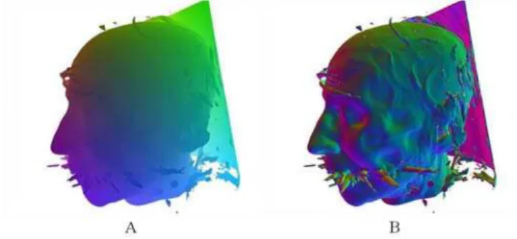
Figure 4.1 Display of a CT-scanned human head data. ... 64
Figure 4.2 The results of HVS. ... 67
Figure 4.3 The results of EMVS. ... 70
Figure 4.4 The results of KMVS. ... 72
Figure 4.5 The results of MSVS. ... 80
Figure 4.6 Diagrams of ATF design and the result of analysing a CT-scanned data ... 83
Figure 4.7 Energy , in active contour algorithm versus the number of iteration ... 85
Figure 4.8 Illustrations of active contour algorithm ... 86
Figure 4.9 Illustrations of a domain of interest initialized in active surface algorithm ... 86
Figure 4.10 Results of active surface algorithm in volume segmentation ... 89
Figure 5.1 Results of constructed lattices based on the segmented information ... 91
Figure 5.2 Diagram of sampling process in MC algorithm ... 93
Figure 5.3 Diagram of the look-up table for surface-edge intersection ... 94
Figure 5.4 Results of extracted iso-surfaces. ... 94
Figure 5.5 Results of extracted iso-surfaces ... 96
Figure 5.6 Results of decreasing sampling rate ... 98
Figure 5.7 Illustrations of adaptive subdivision method ... 99
Figure 5.8 Illustrations of vertex decimation method ... 100
Figure 5.9 Illustrations of vertex merging method ... 101
Figure 5.10 Illustrations of vertex adaptive subdivision solution ... 104
Figure 5.11 Illustrations of deformed control lattices ... 104
Figure 6.3 Mesh-based mass-spring system ... 111
Figure 6.4 Diagrams of decomposing the applied force in mass-spring system ... 113
Figure 6.5 Results of lattice deformation with mass-spring system. ... 114
Figure 6.6 Results of lattice deformation with different stiffness coefficients ... 116
Figure 6.7 Diagram of mapping process deployed in the DOGME ... 117
Figure 6.8 Diagram of I-DOGME ... 118
Figure 6.9 Diagram of improved mapping process deployed in the I-DOGME ... 120
Figure 6.10 Results of volume deformation with different stiffness values ... 120
Figure 6.11 Results of clipped results after the mapping process ... 121
Figure 6.12 Diagram of relationships between control vertices and underlying voxels .... 121
Figure 6.13 Diagram of creating the octree-based lookup function ... 122
Figure 6.14 Diagram of using the octree-based lookup function ... 122
Figure 6.15 Diagram of the arrangement of 8 partitions ... 123
Figure 6.16 Diagram of an digital nested relationship to present the octree structure ... 123
Figure 6.17 Diagram of generating internal relationship for indexing operations ... 126
Figure 6.18 Results of volume deformation with different parameter settings ... 126
Figure 6.19 Results of fixed volume deformation ... 127
Figure 7.1 Diagram of hierarchical structure in CUDA programming model ... 133
Figure 7.2 Diagram of CUDA-based volume rendering pipeline ... 134
Figure 7.3 Illustrations of cubic sampling region ... 136
Figure 7.4 Diagram of CUDA-based lattice construction ... 139
Figure 7.7 Results of octree-based lookup function ... 146
Figure 8.1 Results of DVR with a 2D TF and the ATF design ... 152
Figure 8.2 Results of the volume data processing module ... 154
Figure 8.3 Results of extracting lattices from the isolated segments ... 156
Figure 8.4 Results of non-physics-based deformation ... 157
Figure 8.5 Results of the IVD method ... 158
Figure 8.6 Comparative results of different TF designs ... 159
Figure 8.7 Comparative results of different implementations ... 160
Figure 8.8 Comparative results of different deformation solutions ... 161
Figure 8.9 Results of deformed behaviours resulting from lattice simplification levels . 161 Figure 8.10 Comparative results of different lattice simplification levels ... 162
Figure 8.11 Various results of IVD method ... 163
Table 4.1 Mechanism of HVS ... 67
Table 4.2 Mechanism of EMVS ... 69
Table 4.3 Mechanism of KMVS ... 72
Table 4.4 Comparison between processing times ... 73
Table 4.5 Comparison among performances of processing different data ... 74
Table 4.6 Comparison among three kinds of clustered results. ... 75
Table 4.7 Comparison between the results of EMVS and KMVS ... 76
Table 4.8 Mechanism of MSVS ... 80
Table 4.9 Mechanism of active surface algorithm. ... 88
Table 5.1 Comparisons between results of decimation and subdivision solutions ... 102
Table 5.2 Comparison between results of decimation and subdivision solutions ... 103
Table 6.1 Mechanism of vertex displacement calculation ... 117
Table 6.2 Mechanism for locating voxel’s sequence number ... 119
Table 6.3 Mechanism for locating grid nodes ... 125
Table 8.1 Results of using KMVS and MSVS to process different data sets ... 153
1/2/3D one-/two-/three-dimensional ATF Automatic Transfer Function
BRDF Bidirectional Reflectance Distribution Function CFD Computational Fluid Dynamics
CSG Constructive Solid Geometry CT Computer Tomography
CUDA Compute Unified Device Architecture CVG Constructive Volume Geometry DIP Digital Image Processing
DOGME Deformation of Geometric Models Editor DVR Direct Volume Rendering
EM Expectation-maximization
EMVS Expectation-maximization algorithm-based Volume Segmentation FEM Finite Element Method
FFD Free-Form-Deformation
HVS Hierarchical clustering-based Volume Segmentation I-DOGME Improved Deformation of Geometric Models Editor IDVR Indirect Volume Rendering
IVD Interactive Volume Deformation
KM K-means
KMVS K-means clustering-based Volume Segmentation
LUT Lookup Table
MC Marching-Cubes Algorithm MIP Maximum Intensity Projection MRI Magnetic Resonance Imaging
MS Mean-shift
MSVS Mean-shift clustering-based volume Segmentation PC Personal Computer
PDE Partial Differential Equation SIMD Single Instruction, Multiple Data SIMT Single Instruction, Multiple Threads TF Transfer Function
Acknowledgements ... I Abstract ... II List of Publications ... III List of Figures ... IV List of Tables ... IX List of Abbreviation ... X Table of Contents ... XII
Chapter 1 Introduction ... 1
1.1 Volume Data Acquisition ... 3
1.2 Volume Visualization and Deformation ... 5
1.3 Research Objectives ... 6
1.4 Contributions to Knowledge ... 9
1.5 Thesis Outlines ... 11
Chapter 2 Review on Volume Visualization Approaches ... 12
2.1 DVR Optical Model ... 15
2.2 Ray-casting Theory and Practice ... 16
2.2.1 Volume Rendering Integral Model ... 17
2.2.2 Tri-linear Interpolation ... 19
2.2.3 Alpha Blending Operation ... 20
2.4 The Shear-warp Model ... 30
2.4.1 Parallel Projection Algorithm ... 30
2.4.2 Perspective Projection Algorithm ... 32
2.5 The Maximum Intensity Projection ... 34
2.6 Volume Shading Techniques ... 36
2.6.1 Monte-Carlo Techniques for Iso-surface ... 37
2.6.2 Volume Scattering ... 40
2.7 Research Objectives ... 41
Chapter 3 Volume Model Manipulation Strategies ... 43
3.1 Volume Clipping ... 43
3.2 Volume Deformation ... 45
3.2.1 Non-physics-based Deformation ... 45
3.2.2 Physics-based Deformation ... 49
3.3 Constructive Volume Geometry ... 54
3.4 Volume Animations ... 56
3.5 Analysis on Current Challenges ... 58
3.6 Design Criteria ... 60
Chapter 4 Volumetric Data Processing ... 63
4.1 Applying Clustering Methods for Classifying Volume Data ... 64
4.1.1 Hierarchical Clustering-based Volume Segmentation (HVS) ... 65
4.1.4 Evaluations of Segmentation Approaches ... 73
4.2 Segmentation Improvement and Cluster Representation ... 78
4.2.1 Mean-Shift Clustering-based Volume Segmentation (MSVS) ... 78
4.2.2 Design of Automatic Transfer Function (ATF) ... 82
4.3 Design of Boundary Extraction ... 83
4.3.1 Active Contour Algorithm ... 84
4.3.2 Region-based Active Surface Method ... 86
4.4 Summary ... 89
Chapter 5 Lattice Construction and Refinement ... 91
5.1 Marching Cubes Algorithm ... 92
5.1.1 Sampling and Vertex Extraction Process ... 92
5.1.2 Triangulation Process ... 93
5.1.3 Automatic Construction and Model-fitting Lattices ... 94
5.2 Lattice Refinement ... 95
5.2.1 Varying Sampling Rates ... 97
5.2.2 Adaptive Subdivision Scheme ... 98
5.2.3 Vertex Decimation Approach ... 99
5.2.4 Vertex Merging Method ... 100
5.2.5 Tests and Evaluations ... 101
5.3 Summary ... 105
6.1.1 Lattice Deformation ... 109
6.1.2 Embedding Mass-spring Mechanism-based Framework ... 110
6.1.3 Implementing Resistance Force Mechanism ... 114
6.2 Displacement Mapping ... 117
6.2.1 Mapping Process Design ... 117
6.2.2 Design of Indexable Inherent Relationship (IIR) ... 118
6.3 Octree-based Lookup Function ... 122
6.3.1 Implementing Octree Data Structure ... 124
6.3.2 Constructing Octree-based Lookup Mechanism ... 124
6.3.3 Accomplishing Volumetric Deformation ... 125
6.4 Fixing Deformation ... 127
6.5 Summary ... 128
Chapter 7 System Integration and Acceleration ... 131
7.1 Preparations of CUDA-based Programming ... 132
7.2 CUDA-based Volume Visualization ... 134
7.2.1 Geometric Modelling Function ... 135
7.2.2 Kernel Sampling Function ... 136
7.2.3 Kernel TF ... 137
7.2.4 Kernel Accumulation Function ... 137
7.3 CUDA-based Lattices Construction ... 138
7.3.3 Kernel Subdivision Function ... 143
7.4 CUDA-based Displacement Mapping ... 145
7.4.1 Kernel Octree-based Lookup Function ... 145
7.4.2 Kernel Mapping Function ... 147
7.5 Summary ... 149
7.5.1 SIMT Architecture ... 149
7.5.2 Synchronizing Kernel Functions ... 149
Chapter 8 Test and Evaluation ... 151
8.1 Efficiency Evaluation on Volume Segmentation ... 151
8.2 Effectiveness Test on Lattice Construction ... 155
8.3 Flexibility Assessment on Interactive Deformation ... 156
8.4 System Run-time Performance Evaluations ... 158
8.5 Summary ... 164
Chapter 9 Conclusions and Future Work ... 166
9.1 Conclusions ... 167
9.1.1 Efficient Volume Data Processing... 167
9.1.2 Adaptive Lattice Manipulation ... 168
9.1.3 Flexible Deformation Control ... 169
9.1.4 GPU-accelerated System Integration ... 169
9.2 Future Work ... 170
Chapter 1 Introduction
In contrast to the “pure” mathematical studies carried out by a small group of elite mathematicians in the 19th century, the so-called applied mathematics had been enjoying great success and public attention since the turn of the 20th century (Gluchoff, 2005). One of the main contributions to this phenomenon is the increased integration of the theoretical and abstract mathematical concepts with other scientific disciplines, such as physics, engineering, economics and even biology (Matsuura, Oharu et al., 2003; Dumas, Druez et al., 2009; Hernandez, Mateos et al., 2009; Britz, Strutwolf et al., 2011). The breakthroughs in those vastly diversified areas were supported by new mathematical tools and theories developed in the first half of the 20th century: statistics, topology and modern integral theory.
The invention and wider spread of modern computer technologies since the second half of the 20th century have further accelerated this trend. For example, stemming from computer graphics, volume rendering has been growing into an important research field in the last two decades (Engel, 2004). Most of the developments of volume visualization and application techniques in the 1980s and 90s had focused on exploring the theoretical and mathematic foundations of the visualization process. Since the mid-1990s, three leading research groups have proposed a series of improvements for PC-grade and efficient volume visualization techniques: the portable visualization clients by the Visualization and Interactive Systems group in the University of Stuttgart (Engel, Oellien et al., 2000); advanced volumetric modelling methods by the Visual and Interactive Computing group in the University of Swansea (Chen and Tucker, 2000), and versatile volume shading designs by the
Scientific Computing and Imaging Institute in the University of Utah (Kniss, Premoze et al., 2003).
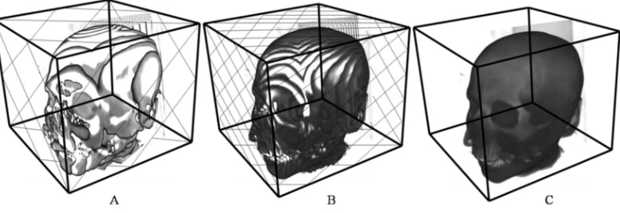
Compared with conventional 3D modelling and visualization techniques, volume models allow direct or indirect access to their internal structures, instead of only showing their surface features. In Figure 1.1, all four snapshots are showing an engine box. Besides the vivid surfaces, wireframe-based model A does not show any internal information. In contrast, model B is a volume model, which can be processed into model C and D respectively to exhibit the interiors via two popular representation modes.
Figure 1.1 An engine box represented via different modes. Model A is a surface model. Model B
presents a volume model; model C shows the internal structure through modifying the optical characters; which model D represents the interiors via the clipping operation.
This visualization technique aims to gain the understanding of multi-dimensional information and to display it as images. Similar to other modelling techniques, it also suffers from a series of challenging problems, such as occlusion within models, random data structures, noisy data, and artefacts generated from display mechanisms. The main objectives of recent researches were to develop solutions for exploring the “visibility” of various volumetric structures (Aykanat, Cambazoglu et al., 2007; Sakamoto, Kawamura et al., 2010). This thesis deepened the understandings by devising a novel solution of which users can freely customize the behaviours of
volume visualization process via interactive manipulation. In this thesis, Chapter 1 starts explaining the volume data source and carry on a brief introduction of two kinds of general volume data acquisition methods. After accomplishing the recapitulative content, the research objectives and the main contributions from the programme will be highlighted at the end of this chapter accompanied by the thesis outline.
1.1
Volume Data Acquisition
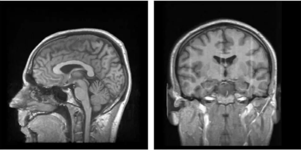
In the 1960s, an American theoretical physicist, Allan M. Cormack, published a mathematical model for calculating different rates of absorption of ionized radiation (i.e. X-ray) when crossing through different body tissues (Cormack, 1979). Based on this model, a British engineer, G. N. Hounsfield, invented the world’s first Computerized Tomography (CT) scanner, an imaging device that allows 2D or 3D sectional or volumetric models to be reconstructed in order to represent internal information from the probed subject (Hounsfield, 1979). Due to their significant achievements, Cormack and Hounsfield won the Nobel Prize in 1979. Figure 1.2 shows the snapshots of a sliced human brain.
Figure 1.2 A CT scan of a human brain
Geometry developed by Johan Radon in 1917 and translated into English in 1986 (Radon, 1986). The Radon transform is widely applicable to tomography, the creation of an image from the scattering data associated with cross-sectional scans of an object. If a function , represents an unknown density, then the Radon transform represents the scattering data obtained as the output of a tomographic scanner. Hence the inverse of the Radon transform can be used to reconstruct the original density from the scattering data, and thus it forms the mathematical underpinning for tomographic reconstruction, also known as image reconstruction.
The Cormack model resolves the inverse Radon Transformation issue through convolution and inverse projection. Therefore, once the , is determined, it is possible to reconstruct the sectional images of the measured tissue. Techniques like Magnetic Resonance Imaging (MRI) may use a less invasive measuring mechanism, but its foundation theory is similar to that for scanned image registering and reconstruction.
Current CT and MRI scanning processes were normally time-consuming and uncomfortable for patients, due to the rigid body postures which need to be maintained throughout the dedicated solutions (Olabarriaga and Smeulders, 2001; Fluck, Vetter et al., 2011). The latest advancements in digital processing have seen fast scanning technologies being developed and utilized with varying degrees of success (Zhou, Matsumoto et al., 2010; Cho, Cho et al., 2012). However, the scanned images often suffer from unsatisfactory qualities (e.g. noise-level) due to their inherent acquisition mechanisms that can cause great difficulties for image and 3D reconstruction (Qian, Joshi et al., 2011). One of the motives for this research is to investigate data filtering (pre-processing) techniques, prior to attempts being made to
improve the performance of the following volume visualization and deformation approaches.
1.2
Volume Visualization and Deformation
After sampling the volume data in a regular sequence, the inherent information can be converted into a series of parameters. The following visualization work can be implemented directly (known as Direct Volume Rendering, or DVR), or accomplished indirectly by relying on an iso-surface and then “copying” the polygonal displaying strategy using surface modelling techniques (called Indirect Volume Rendering, or IDVR). In order to explore the various features inside the volume data, a special Lookup Table (LUT) is utilized for the purpose of data classifying, and to “individualize” them with associated values. These values are to be accumulated together on the image plane so that the inherent information can be represented via an understandable image.
As a process for manipulating volume models, volume deformation can be categorized as both non-physics-based and physics-based (Correa, Silver et al., 2010). The former techniques were well-known because of the ability to “freely” deform volumetric objects. In associated deformation applications, there was little or no regard to the consideration of physical realism (Forsberg, Mooser et al., 2008; Sugihara, Wyvill et al., 2010). In contrast, physics-based techniques are strictly governed by the result of utilizing physical equations to calculate the external and internal forces (Nealen, Müller et al., 2006; Bordemann, 2008). As the line between these non-physics-based and physics-based deformation approaches is becoming blurred in surface modelling techniques, more and more researchers are trying to use non-physics-based techniques to produce the physical effects in volume-based
applications (Correa, Silver et al., 2010). However, most of them relied heavily on man-made constraining operations and one-sided assumption-based works, which had undoubtedly caused many artefacts and imprecise outputs during the “real-life” simulations.
This thesis referred to physics-based volume deformation as a technique whereby deformation was driven explicitly by applying forces on the control lattices enclosing the volume model. In addition, both inertia and internal forces were considered. This deformation method aims to describe the deformation behaviours and exhibit the internal transformation precisely.
As an important criterion for evaluating deformation techniques, the performance of interactive operations always influences the development of volume deformation (Yuan, Zhang et al., 2010). The requirement for “on-the-fly” mechanisms exists at every stage of the deformation pipeline, such as the sampling, transforming and final displaying stages. In particular, the physics-based methods rely on complicated calculations in order to provide precise deformation results, and consequently physics-based manipulations of the volume model will lead to an inconceivably time-consuming data processing. As a result, the physics-based volume deformation requires hardware-based acceleration techniques to maintain a higher interactive rate during the simulation.
1.3
Research Objectives
It is a common scenario that when deploying volume-based operations, the involved complex data sets are often of 10 times scale, as compared to the surface-model-only implementations, which leads to a heavy workload of sampling and rendering
operations for the host computer. The major development of the computing platform took place at the turn of the new Millennium empowered by the rapid consumer grade computer (see Appendix B) evolution (some reckoned as a revolution) (Mark, Steven et al., 2003). As a result of this, complex scientific simulation and visualization tasks have started moving from expensive workstations to Personal Computers (PCs). The current consumer grade computers can support many complicated graphical and non-graphical modelling at a near interactive rate through larger memory storage, broader data bus and faster data access. Volume visualization and its applications are among the first to benefit.
Accompanied by the increasing computing power supplied by the innovative hardware platforms, volume models and their derived manipulations are quickly coming out of the shadow of the surface models and becoming one of the main representation forms for special applications (Strengert, 2005; Tatarchuk, Shopf et al., 2008). Although there were still many challenges in volume visualization and application techniques, i.e., in the real-time interaction arena, many research designs have been focusing on improving the efficiency of the volume-based applications, enhancing the rendering quality, or developing the interactions with the volume models.
In addition to directly rendering, volume models can support other processing methods so that more intrinsic information can be acquired, e.g. clipping methods. This project created a novel volume deformation mechanism which enabled precise representations of the deformation behaviours, rapid interactive operations and versatile applications. The aim and objective of this project can be summarized as follows:
To investigate the state-of-the-art of volume visualization and deformation techniques. The evaluation criteria were summarized based on the literature review and used to discuss the pros and cons of the implemented system. The system performances were categorized into three terms: “Flexibility”, “Efficiency”, and “Accuracy”, of which the evaluations were respectively estimated through processing different volume data, counting the real-time performance and tackling customization operations (Correa, Silver et al., 2010; Patete, Iacono et al., 2012).
To improve the system performance. Besides the help offered by GPU-based acceleration designs, the solution also comprised the dedicated data processing strategy designed for solving the problem of large volume data size (Cates, Lefohn et al., 2004). By studying the classic Digital Image Processing (DIP) methods, this project finished a high-dimensional DIP solution for carrying out volumetric data classification and information extraction (Fang, 2001).
To accomplish the physics-based deformation mechanism for manipulating volumetric features. First of all, a mathematic model was constructed for partitioning the resulting deformation behaviour into a set of changed characters within the volumetric space (Bachmann, Bouissou et al., 2009). Secondly, the assignment of these characters was based on an order which records the nested structures inside the volume model. And the control lattices met the demands: nonexistence of self-intersecting polygons, this “model-fitting” lattice conforming to models’ surface features, and the adaptive meshwork structure (Sauvage, Hahmann, et al., 2008). In addition, the data exchange between CPU and GPU were investigated for further efficiency gain (Lefohn, Kniss, et al., 2003).
1.4
Contributions to Knowledge
Besides the literature review, the main research efforts discussed in this dissertation were respectively reflected by four functional modules (as shown in Figure 1.3). As a result, the contributions to knowledge from this project can be summarized as:
Figure 1.3 A diagram of the design system pipeline
Volume data segmentation abstracted interesting information from the continuous volume data; meanwhile, filtered out the inherent noise and the trivial segments, and consequently avoided useless data computation and processing tasks. Instead of processing the resulting images, or relying on per-frame-based operations, the strategy of volume data segmentation created a one-off 3D data pre-processing before progressing visualization and deformation operations. It was published in the 17th ICAC conference paper. By rendering these segment data, the result directly exhibited the internal structure which can offer help in choosing the interesting data segment(s).
In order to customize the extent of transformations, the spatial determination process relied on two key designs. One was a lattice-based “interface” between applied forces and underlying volume models. The outcome of the lattice construction process can influence the results of deformation operations. One was a tree-like framework for ascertaining whether the voxels belong to the deformed domain. Both them were explained in the same paper.
The spatial displacement response within volume models was derived from similar surface-modelling-based deformation examples, which styled the external force calculation. And the deformation process was “translated” into a set of parameter computations through determining a special data structure to standardize the transformation operations. As a result of this, the parameter calculation and data accessing tasks can be accelerated by the GPU-based parallel computation design, so that the interactive rate of future operations can be optimized. The benefit from GPU-accelerated achievements was firstly mentioned in my paper published in 16th ICAC conference.
Similar to the conventional displacement mapping techniques for mesh-based object deformation, the voxel displacement map was designed to record voxels’ offset distances. This project utilized the view-aligned proxy geometry for volume data storage, therefore, the voxel displacement map was correspondingly 3D-based. This 3D texture mapping avoided the complicated interpolation processes involving the combinations of 2D and 3D textures, and consequently improved the system efficiency. This part is based on the work document published in 15th ICAC conference.
By harnessing the parallel processing capabilities of GPU, the hardware acceleration design in this research managed data through synchronizing each sub-tasking. Therefore, the visualization and deformation operations were partitioned into a set of subtasks synchronized in a parallel structure for improving the system efficiency. This design was explained in the 17th ICAC conference paper.
1.5
Thesis Outlines
A comprehensive literature survey regarding contemporary volume visualization methods is recorded in Chapter 2. Chapter 3 provides an in-depth discussion on the strategies of manipulating volume models, as well as the state-of-the-art in volume deformations. The actual research methodology, design approach, implementation strategy and evaluations are respectively covered into four chapters. Chapter 4 employs image segmentation methods and improved them for classifying volume data. The classification enables the display of internal structures of complicated volume data and the extraction of interesting data segment(s), which in turn, simplifies the workload of the following data processing activities. The content in Chapter 5 explains the lattices construction’s design principles and working mechanisms for enclosing the manipulated volume data. As a vital part of this physics-based volume deformation system, the constructed lattices met various pre-defined requirements, such as the “model-fitting” lattice, flexible modification and rapid construction. Chapter 6 covers the implementation of the deformed volume models. A mathematical model has been established to subdivide the deformation behaviour into the displacements of voxels through a “deformation parameterization” operation. Chapter 7 reveals the details of the Compute Unified Device Architecture (CUDA)-based implementations of the system prototype. This programming model was used to separate the lattice construction and deformation parameterization processes into sub-computation tasks, and to synchronize them into a parallel computing architecture for the acceleration purpose. Chapter 8 uses the common evaluation criteria to access this deformation system in terms of its intermediate results, real-time performances, rendering quality. Chapter 9 concludes the research with achievements and future work.
Chapter 2 Review on Volume Visualization Approaches
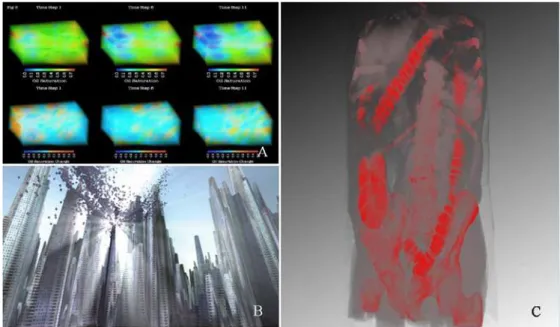
In early 1980s, volume visualization started attracting discussions in scientific communities, due to its potential and powerful capabilities in revealing the internal structures of objects (Drebin, Carpenter et al., 1988). However, limited by the computational methods and platforms at the time, volume visualization and deformation techniques faced tough challenges in various types of practical applications (as shown in Figure 2.1), especially in real-time operations. In the last decade, various research and pilot projects had focused on improving the quality of the final rendered results; meanwhile, maintained adequate performances in real-time operations (Kruger and Westermann, 2003; Strengert, Magallon et al., 2005; Tatarchuk, Shopf et al., 2008; Fluck, Vetter et al., 2011).
Figure 2.1 Various applications of volumetric information. Image A is for studying oil reservoirs
in underground rocks (courtesy to Paul et al.). Image B illustrates a volumetric lighting method for gaming scenes (courtesy to Nvidia Corporation). Image C exhibits a torso model for the medical applications.
From this review of volume visualization terms, a comprehensive introduction of various visualization approaches can be accomplished with potential challenges in different applications. Based on this review, the research problems can be concluded and chosen as the objectives for developing visualization properties.
Volume visualization techniques represent the object via displaying its spatial characters in the form of images. Between the data acquisition and visualization stages, there exists a modelling process which fills a 3D space (as shown in Figure 2.2 (A)) with a set of 3D geometrical elements in order of the original data’s inherent sequences. Each data can be assigned to a cubic element which is regarded as a volumetric pixel, and therefore named as “Voxel”. All voxels (as shown in Figure 2.2 (B)) can be accessed in the form of partitions inside of the volumetric space (as shown in Figure 2.2 (C)). Each voxel can provide two types of parameters: one is 3D coordinates defined via its spatial location, and the other is a scalar value derived from the raw volume data. Depending on different voxel processing approaches, volume visualization can be categorized into direct (DVR) and indirect (IDVR) strategies.
Figure 2.2 Illustrations of volume model formations
IDVR methods use vertices to replace voxels for indirectly representing the volume data. Marching-Cubes (MC) algorithm is a prevalent IDVR, which consists of following operations: extracting vertices from the volume data, grouping them
according to their scalar values, and implementing the Delaunay triangulation for each group of vertices (Lorensen and Cline, 1987) . This algorithm and output images will be covered in Chapter 5.
On the contrary, DVR solutions carry out a series of direct operations on voxels. These visualization algorithms require a pre-defined optical model for managing the conditions of volumetric light emission, light scattering, light absorption and ambient occlusion among voxels. These physical quantities are all based the voxels’ optical properties which are notionally determined by their scalar values, and will be numerically represented by a series of RGBA quadruplets after the sampling process. This process of converting scalars into colours is yielded by the so called “Classification” phase.
The next step is sampling these values by casting a set of (parallel) rays through the volumetric space. Depending on the different directions of these rays, DVR methods can be divided into backward-mapping and forward-mapping ones (shown in Figure 2.3) (Engel, Hadwiger et al., 2004). In forward-mapping approaches, the voxels forward project themselves onto the image plane, to compose the final image via a sort of pixel distribution. Backward methods regard the viewing rays as sampling tools, which penetrate through the pixels in the image plane and detect the voxels’ parameters for the image synthesis process. Because the system introduced in this thesis mainly relied on backward-mapping DVR in the visualization phase, the review of volume visualization techniques only focused on the forward-mapping methods. Consequently, without any additional explanation, the directions of DVR techniques discussed in the following context are all backward-oriented. As an important part of the image synthesis process, calculating the light propagation via the integrating light
interaction effect for each point within a volumetric space is based on the choice of optical models.
Figure 2.3 Diagrams of forward-mapping and backward-mapping methods
2.1
DVR Optical Model
An optical model serves as a paradigm that composes lighting-emitting points of uniform physical quantity. Based on different conditions of light propagation inside a volumetric space, the optical models can be classified as:
Absorption only. This type of optical model determines the volumetric space to be a kind of black hole. In this region, all lights are completely absorbed, and consequently unable to support emitting or scattering conditions (as shown in Figure 2.4 (A)).
Emission only. In comparison to the absorption only model, which prevents light emission and scattering, the emission-only optical model just focuses on the light emission condition, without any consideration of absorption or scattering (as shown in Figure 2.4 (B)).
Absorption plus emission. As a syntheses of the above two optical models, this model simultaneously enables light emission and absorption. Because most DVR-based applications always overleapt the discussion of scattering and indirect illumination, the absorption plus emission optical model is the most popular choice for volumetric light propagation (as shown in Figure 2.4 (C)). Scattering and shading. Using this optical model, the light scattering can be
treated among the particles at voxel level. The scattering condition comprises projecting lights onto the surface of each voxel from a light source without any impeded objects, and being generated by the occlusion states among the voxels (as shown in Figure 2.4 (D)).
Multiple scattering. As an extension of simulating light scattering in a volumetric space, the multiple-scattering optical model allows performances of the complicated mechanism of an incident light scattered by multiple voxels.
Figure 2.4 Shading results determined by different optical models
2.2
Ray-casting Theory and Practice
The ray-casting displays mechanism was summarized as sampling 3D information (voxels) and rendering in 2D formats (pixels), which belonged to the image-order rendering method (Ray, Pfister et al., 1999). Besides, the texture mapping approach,
which decomposes a volumetric space into the given type of slices (2D or 3D), was classified as an object-order rendering method (covered in section 2.1.3) (Weng, Lin et al., 2002).
As the most direct solution for evaluating the volume rendering integral along the rays from image space to object space, ray-casting was defined as the most basic DVR algorithm and a kind of backward-mapping approach (Levoy, 1988; Choi, Shin et al., 2000). After sampling the voxels’ optical properties via casting (parallel) rays in the viewing direction through pixels into the volumetric space, ray-casting accumulates the resulting properties for each ray in the form of evaluating the volume rendering integral and rendering the results in the manner of pixels in the final display.
2.2.1 Volume Rendering Integral Model
In every volume rendering method, the volume rendering integral was always evaluated in a certain direction. Generally, the viewing ray was chosen for evaluating the integral, even if it was unclearly defined. Because the sampling mode was not continuous in practice, the related optical properties were not continuous either. In order to approximate the evaluation of the volume rendering integral, the calculation was digitally replaced by a Riemann sum, which performs the accumulation of the properties along the viewing ray in terms of colour values (Levoy, 1988).
Each viewing ray will, of course, penetrate through a number of voxels in certain statuses including through a voxel’s centre, through a voxel and on one of six tangent planes of it. The simplest condition is traversing through a voxel’s centre so that its scalar value can be directly used as the sampled result of the viewing ray at this voxel. For the other two statuses, the sampled results all need to be calculated via the tri-linear interpolation in ray-casting-based applications (or 2D interpolation for
texture-based processing).
After the sampling process, the scalar value of voxel can be gained for the following calculations. The indicated a voxel which is sampled by the _ viewing ray at a distance along this ray to a virtual viewpoint (as shown in Figure 2.5). This vector-based parameter comprised the information for indexing the scalar values stored in a kind of texture memory. When the most popular optical model (absorption plus emission) is employed, the indexed scalar value is represented via a colour value called emissive colour, and the absorption coefficient is defined for describing the condition of light absorption via
. It can be written as (Engel, Hadwiger et al., 2004):
· (2.1)
Based on these two kinds of colour values, the volume rendering integral can carry out the resulting composition of colour values sampled along the rays. For example, in order to calculate the result of the viewing ray passing through a distance (shown in Figure 2.5), the absorbed and emissive colours at different locations can be worked out respectively.
Figure 2.5 A diagram of a viewing ray for volume rendering integral
First of all, it is assumed that there are voxels detected on this ray and no intervals between any two neighbouring voxels. Based on the equation 2.1, for the constant
absorption coefficient , the light absorption on this ray can be written as:
· · · , (2.2)
On the condition that is dynamic, and depending on its position, the equation 2.2 will be changed into:
· · · · , (2.3)
In the same way, the corresponding light emission can be represented via
· ( , ). After finding the related and ,
the final result of this voxel on the image plane is , which can be written as:
· · · (2.4)
2.2.2 Tri-linear Interpolation
Tri-linear interpolation was usually utilized to implement a multivariate interpolation for generating the sampling result in a voxel whose centre cannot be penetrated through by a viewing ray (Engel, Kraus et al., 2001). The tri-linear interpolation locates the resulting point with its scalar value through weighting eight neighbours’ coordinates and their scalar values (Rajon and Bolch, 2003). For example, as shown in Figure 2.6, the Viewing ray needs to gain the scalar value of the point . After knowing about the scalar values of ’s eight neighbours ( ), the first cycle of tri-linear interpolation locates the new generated points ( ). Based on these points, the send cycle of the interpolation locates the point , and returns its scalar value as the final output. Because of the capability of calculating
the interpolated values, the tri-linear interpolation is applied to “filter” ambiguous representations, and avoid visual artefacts caused by limited inputs with intervals between data, or inaccurate results because of discontinuous samplings.
Figure 2.6 A diagram of tri-linear interpolation
2.2.3 Alpha Blending Operation
After obtaining in equation 2.4 and finishing the associated explanations of interpolation processes, an integral part of volume rendering is to carry on the composition operations in the alpha blending process, which accumulates colour values in the back-to-front or front-to-back order. The example shown in Figure 2.5 is a front-to-back approach, i.e., its composition starts at the voxel closest to the image plane and ends with a given voxel.
The composition process accumulates the sampling values in an opacity-weighted calculation, which is obtained by pre-multiplying the original value by its associated opacity property: alpha value. In this front-to-back method, , which represents each step of the composition, starts at and accumulates the result of multiplying the _ voxel’s value by the corresponding alpha value (Wittenbrink, Malzbender et al., 1998):
, , (2.5)
This alpha value is related to the voxel’s location and the theory can be written as (Blinn, 1994):
, , (2.6)
which means that the alpha value is determined by its previous one and the alpha value of the sampled value at this point is . Then the calculated is loaded in the equation 2.5 for the composition calculation.
By iterating the calculation in equation 2.5, the volume rendering integral on the _ ray is calculated via the Riemann-sum-based composition (Engel, Hadwiger et al., 2004):
∑ ∑ (2.7)
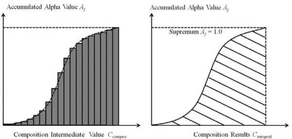
Playing the role of controlling the supremum in the Riemann-sum-based volume rendering integral, alpha blending can determine the terminal of composing colour values in the front-to-back method. The composition can define an optimal indicator (known as early-ray-termination), which determines the progress of alpha blending. As shown in Figure 2.7, when the cumulated alpha value (yielded in equation 2.6) is equal to 1.0, the result of the Riemann-sum-based composition will stop at the current position.
Figure 2.7 Diagrams of colour accumulation (left image) and approximated volume rendering integral (lined shadow area in right image)
is the final result of the _ ray after passing through the volume rendering integral, and represented by a few pixels which are stored in the frame buffer in the form of 2D texture. The resulting images are shown in Figure 2.8.
Figure 2.8 The results of ray-casting
However, as a number of image-order algorithms suffered from low efficiency caused by redundant computations, every ray-casting-based application struggled against the same challenges that the occasioned heavy sampling work on every ray and the iterative computations of opacity composition (Ray, Pfister et al., 1999). To overcome these drawbacks, the researchers mainly focused on developing an orientated rendering mode (e.g. digital boundary determinations to highlight or conceal given
regions) (Leu and Chen, 1999), increasing the efficiency of sampling mechanisms (e.g. early ray determinations to manage the progress of sampling every ray) (Hadwiger, Sigg et al., 2005), and improving display capability with the aid of applied hardware (e.g. high-quality performance of multiple volumes to enable realistic displays within complicated environments) (Tatarchuk, Shopf et al., 2008). In addition, there were a series of hybrid-based solutions that combines the image-order and object-order algorithms together to overcome their inherent disadvantages whilst, furthermore, maintaining their respective advantages for improving the performance of these solutions (Westermann and Sevenich, 2001).
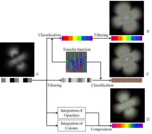
2.2.4 Classification Process
Classification process relies on Transfer Function (TF) for assigning optical properties (colour, opacity, etc.) to the voxels by indexing their scalar value in a colour-based lookup-table (Engel, Hadwiger et al., 2004). Different combinations of the classification and the interpolation-based filtering processes will make the results of visualizing the same model totally different. The alternate order between classification and filtering processes respectively forms pre- and post- classification methods, and produces two kinds of results (as shown in Figure 2.9 (B and C)). Image D is an output of the pre-integrated classification design. Besides the visual artefacts in their results, all visualized features can be fully represented based on the complicated design of Nyquist frequencies in the TF design which always limited the real-time performance of visualization applications (Arens and Domik, 2010).
Figure 2.9 Diagrams of pre-, post- and pre-integrated classifications
For overcoming these limitations, an advanced solution was proposed to use the numerical integration to replace the complex Nyquist frequencies in the TF design (Engel, Kraus et al., 2001). Its idea is to “linearize” the sampled volume data into a whole segment which comprises a stat point and ends with the last sampled data. The information of this segment needs to be integrated before the classification, so-called pre-integrated classification. In this solution, the length of the segment will be increased as the sampling work proceeds. The integration will keep a non-stop update on the colour and opacity of this segment. This integration requires two simple TFs for colouring the segment and voxels respectively.
As shown in Figure 2.9, the integration operation consists of two steps. The integration is for calculating the opacity of a segment. The other one is for integrating the sampled voxels’ colour values. The integrated opacity of this segment can be written as (Engel, Kraus et al., 2001):
exp (2.8)
where represents a voxel’s scalar values, is a simple TF for transforming voxels’ scalar values , and is the number of voxels covered in this segment (the distances between voxels are assumed to be zero). The other integration is for the colour value of the segment can be written as:
exp ′ ′ (2.9)
with the other TF for colouring the segment. Besides avoiding the complex Nyquiest frequencies in pre- and post- classification approaches, the pre-integrated classification can generate high quality visual results (as shown in Figure 2.9(D)).
TF had also attracted a great deal of attention on its multidimensional-based applications. In volume-based applications, as the simplest method, 1D TF directly maps the voxels’ scalar values to associated colours and opacities. But, it cannot differentiate between volumetric subspaces whose voxels share the same scalar value but belong to different regions, e.g. the skull and teeth segments in a CT-scanned human head data. In order to solve the problem of inadequate representations in 1D TF, more parameters were utilized as the other dimensions in the TF (Arens and Domik, 2010). Besides the scalar value, a 2D TF can use the gradient magnitude as the second dimension for determining the differences between these domains (Levoy, 1988; Konig and Groller, 2001). The magnitude of gradient is used to represent the sampling statues. For example, there won’t be any change when sampling within a volumetric subspace, and the sudden change of gradient will happen when the current location of sampling is outside of the subspace (Kniss, Kindlmann et al., 2002).
Another 2D TF uses the curvature of volumetric subspaces as the second dimension. Generally, the shape of each volumetric sub-space contains a unique combination of the most and least curvatures (Hladuvka, Konig et al., 2000). Therefore, this 2D TF can differentiate complex volumetric information. Due to its capability of shape discrimination, this curvature-based TF usually serves as a shape-based analysis in the surgical simulations (de Vaal, Neville et al., 2011).
Besides the above TF design, 2D TF techniques also use the other available properties as the second dimension, such as distance-based method is based on the radiation radius of a pre-decided point (Tappenbeck, Preim et al., 2006), size-based TF uses the scale space for detecting the sizes of object domains (Correa and Ma, 2008), texture-based method relies on the texture analysis which detects the change of texture properties for mapping given specific opacities and colours to voxels (Caban and Rheingans, 2008). With voxel’s scalar value, each of these available properties is used to form a multivariate control which enables the 2D TF methods to reveal more features than 1D methods (Kniss, Kindlmann et al., 2001; Kotava, Knoll et al., 2012).
Due to the increasing number of dimensions, multidimensional TF applications need to simplify the huge workload of manual assignments. Different from the complex trial and error tests in the multidimensional TF techniques, the automatic and semi-automatic methods all depend on the pre-defined criteria for driving the mapping operations (Pfister, Lorensen et al., 2001). Automatic TF designs are good at maintaining the interactive rate to real-time applications (Petersch, Hadwiger et al., 2005). Semi-automatic methods emphasise the importance of the user’s intuitions and the flexibility of keeping a few manual modifications according to given conditions (Pinto and Freitas, 2008). The criteria can be categorized as two types: image-driven
and data-driven. Image-driven TF techniques usually focused on the quality of visual results and estimates the optimal design via a series of parameterized criteria (Pinto and Freitas, 2006; Park and Bajaj, 2007). Data-driven methods generally concentrate the capability of precise data displays, e.g. identifying the boundaries between volumetric sub-spaces (Kaul, 2010).
2.3
Texture-mapping Approaches
Figure 2.10 The results of object-aligned slices
Initially, texture-mapping plays a “skinning” role in surface modelling techniques. It serves to map visual features onto the surfaces of vertex-based frameworks, in order to represent the appearance of surface models. Mostly, these features are stored and processed in the form of 2D texture, so this displaying technique is named texture-mapping. In voxel-based environments, the volume data set is represented via a set of 2D textures, and anticipates the composition in the form of texture-based units. Unlike the ray-casting method (which belongs to the image-order method), texture-based volume visualization is an object-order method, and its displaying
quality is mainly dominated by the texture arrangement design (Engel, Hadwiger et al., 2004). In primitive texture-based volume rendering applications, three stacks of slices (textures), so-called object-aligned slices, respectively performed the view of a volume model in X-, Y- or Z-axial directions (as shown in Figure 2.10).
In associated applications, these slices were all pre-constructed, with the intention of determining one stack once for given conditions, such as the spatial attitudes of the volume object with a fixed viewpoint, along with orbit orientations of the viewpoint and complicated combinations of these two conditions. After finishing the slice-based representation phase, the following composition phase plays a “mapping” role, displaying the final results after implementing the integral calculations and the blending process slice by slice. Shear-warp model is a typical example of the object-aligned slices. Its mechanism of the composition process and operations will be explained in the section on shear-warp model below.
Because every slice is a potential candidate in 2D texture-based applications, producing the final display results generally requires the execution of the sampling, filtering (interpolation) and blending process three times for a proper representation. Besides the trebled workload, another manifestation of its disadvantages is the complicated pre-definition of the conditions for the slice exchange. Although this texture-based method manages to suffice for regular volume rendering applications, the above listed inconveniences restrict its performance in high-quality display applications.
For non-hardware accelerated techniques, texture-mapping-based volume rendering methods have always lost in most competitions with image-order methods (Weiskopf, Hopf, et al., 2001). By the 1980s, progressive graphics hardware techniques made a
great leap in terms of texture-based data manipulation, and consequently texture-mapping-based techniques attracted intensive attention. Benefiting from these advancements, texture-based applications obtained an increasing competitiveness in visualization, in comparison to other visualization methods. Meanwhile, an advanced texture-mapping method, so-called view-aligned slices, which constructs a one-off texture-based representation for replacing 2D textures, was proposed to save the predefinitions of the conditions with its developed texture representations (shown in Figure 2.11).
Figure 2.11 Results of view-aligned slices. From Image A to Image C, the sampling rate is
gradually increased.
However, the display qualities of both 2D and 3D texture-based volume rendering are all limited by the frequency of the slicing volume data sets. For example, both column-II in Figure 2.10 and image B in Figure 2.11 show visibly discrete regions in the final results because of the incorrect initialization of the slices’ properties. By increasing the number of slices, the resulting display can minify these interruptions so that a smooth look is produced for the naked eye (column III in Figure 2.10 and image C in Figure 2.11). Besides these usages, texture-based representation also plays an important part in implementing the shearing-warp model.
2.4
The Shear-warp Model
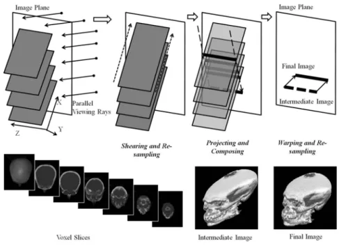
The shear-warp model makes the voxels project themselves, and consequently replaces casting rays into the volumes. The main objective of this forward-mapping approach is to simplify the complicated interpolations and compositions caused by transforming 3D properties into 2D results in an arbitrary kind of transformation (Levoy, 1994). Its basic idea is to shear and warp the volume model in the form of a fixed stack of slices, so that a 3D composition of the voxels’ properties can be approximated via a 2D solution. Its potential customers are the applications which require a lower sampling accuracy and display quality than those of high-quality approaches. Depending on the different types of viewing mode, the shear-warp model is respectively optimized for parallel projection and for perspective projection.
2.4.1 Parallel Projection Algorithm
Figure 2.12 A diagram of the shear warp model with the parallel projection mode
As shown in Figure 2.12, the parallel viewing rays penetrate the image plane perpendicularly. After slicing the volume data, the shearing operation manipulates
these slices perpendicular to the viewing rays. Essentially, the sheared slices can parallel the image plane. In Figure 2.12, an intersection angle is forcedly drawn between slices and the image plane, in order to highlight the condition that the directions of the projecting intermediate image and the final image are not coplanar.
Because the shearing operation was along the Z-axial direction in this figure, the z-coordinate can be kept constant. In other words, the original locations of voxels on each slice all obtain the displacements in the (x, y)-plane. Therefore, the shearing operation can be expressed by:
(
∆ ∆ ) (2.10)
where means the original coordinate matrix, represents the sheared result and is a defined shearing matrix. The ∆ and ∆ respectively mean the X- and Y-axial displacement of voxels on the _ voxel slice. Then, the sampling process will follow the calculated and the sampled results are composited along the Z-axis. Unlike the 3D composition of voxels’ optical properties in the ray-casting method, the shear-warp model carries out the composition by taking each slice as a unit. Therefore, the results of viewing rays intersecting the slices can be approximated via a series of scan-lines, which consist of voxels with the same z-coordinate. In the same way, the tri-linear interpolation in ray-casting methods can be replaced by the bi-linear one. Therefore, the interpolated properties of voxels can be also treated as scan-line-based (as shown in Figure 2.13), and calculated for compositions.
Figure 2.13 A diagram of interpolating scan-lines
The composition of sample results is then projected as an intermediate image. However, this image is also sheared (shown in Figure 2.12). Before being mapped onto the image plane, the warping operation is required to restore the sheared image. In order to implement a reverse calculation on the intermediate image, the warped result can be written as (Levoy, 1994):
(
∆ ∆ ) (2.11)
Through this warping operation, the stored image can be mapped onto the image plane.
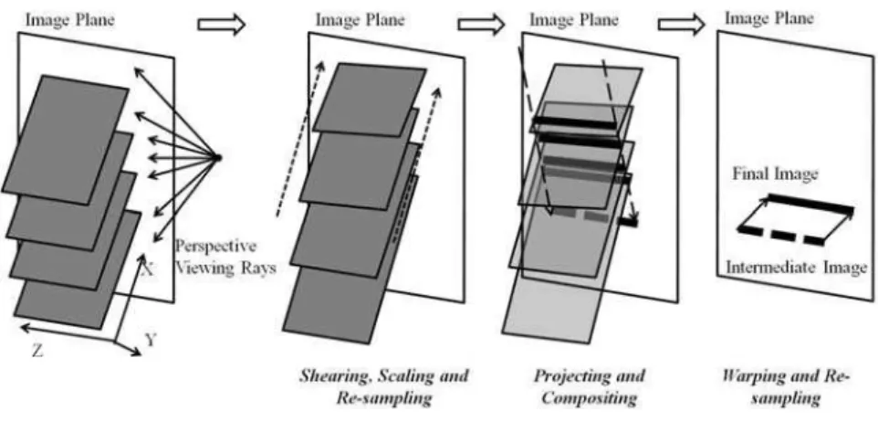
2.4.2 Perspective Projection Algorithm
In order to shear the volume object for the perspective projection condition, the slices need a combination of shearing and scaling operations to implement a similar projection transformation to that which exists in the viewing frustum in Figure 2.14.
This shearing operation is converted into (Levoy, 1994):
∆ ∆ (2.12)
In the viewing frustum, means the distance between the camera and the origin of the viewing space. In this shear-warp model, is designed to control scaling slices after shearing terms, and the scale is . In the same way, the warping operation is (Levoy, 1994):
( ∆
∆ ) (2.13)
Therefore, the result of the shear-warp model with perspective projection can be obtained. Because perspective and parallel projections all rely on the same composition, interpolation and sampling mechanism, both the final images of these two algorithms are the same.
As a complement to high-quality rendering methods, shear-warp model authentically simplified the interpolation and composition tasks required in the volumetric texture-mapping techniques through using one stack of slices for various conditions. Research of shear-warp model mainly focused on the improvement of TF to improve the efficiency of transformation properties, exploring the trade-off between online
shading management and performance penalties, and experimenting with the feasibility of the coexistence with other object-order methods (Wu, Bhatia et al., 2003).
2.5
The Maximum Intensity Projection
Unlike the compositing of optical properties in the ray-casting and shear-warp approaches, Maximum Intensity Projection (MIP), which is a backward-mapping DVR approach, keeps the maximum property value encountered along a viewing ray as the ray’s final footprint projected on the image plane (Wallis, Miller et al., 1989). Its most popular applications were in the field of medical imaging, with its capability for computationally fast imaging, such as cancer screening equipment, CT scanners and diagnoses in nuclear medicine. As shown in Figure 2.15, the MIP’s composition work can be considered as a texture-based method. However, its differences from the other texture-based techniques are the textures parallel the viewing ray.
Figure 2.15 A diagram of MIP
By carrying out the maximum operator along one side of each slice, the final result of MIP can be considered as a set of projections of slices which are perpendicular to the
image plane. The projection of each slice can be written as (Wallis, Miller et al., 1989):
, , , , , , … (2.14)
where , , denotes the property value encountered along the _ viewing ray through the _ slice; , symbolizes the location of the associated footprint on the image plane, and ( , ) is the optical value of the voxel at coordinate ( , , ). Figure 2.16 shows the result of MIP technique.
Figure 2.16 Results of MIP
The mechanism of MIP determines that each pixel value in the result is obtained by locating a maximum optical value. This result cannot support an adequate depiction of the spatial content of overlapping regions, because of the lack of “depth information”. As one general solution for creating MIP-based animations (e.g. rotation), an illusion is pre-constructed by determining the location of a set of viewpoints, and using the slice-based transformations in shear-warp model to obtain the associated image of