New Approaches in Network Data Analysis
Dissertation an der Fakult¨at f¨ur Mathematik, Informatik und Statistik der Ludwig-Maximilians-Universit¨at M¨unchen
New Approaches in Network Data Analysis
Dissertation an der Fakult¨at f¨ur Mathematik, Informatik und Statistik der Ludwig-Maximilians-Universit¨at M¨unchen
Zweiter Berichterstatter: Prof. Dr. Christoph Stadtfeld Dritter Berichterstatter: Prof. Dr. Christian Heumann
I would like to thank Prof. Dr. G¨oran Kauermann for his support, supervision and positive attitude during the problems we sometimes had submitting a paper. Thank you for giving me the opportunity working in this exciting research field and for encouraging me throughout the years. I appreciate a lot that you gave me the time and support being with my little boy.
I thank Prof. Dr. Christoph Stadtfeld for taking the time to come to Munich and being my second reviewer.
I would like to thank Prof. Dr. Christian Heumann for serving as a reviewer and for the good time during choir practice. Furthermore, thank you for supervising me in my Bachelor thesis and consulting project, which encouraged me to continue.
I would also like to thank
. . . Prof. Dr. Volker Schmid for serving as chair for my disputation and Prof. Dr. Thomas Augustin for being available as a backup reviewer.
. . . Prof. Dr. Helmut K¨uchenhoff for hiring me at the StaBLab and introducing me to the work at the university.
. . . Eva and Christoph for sharing the office with me in a calm and friendly atmosphere.
. . . Gunther, Tina, Linda and Andi for the fun lunch and coffee breaks, vacations and good times on mountain tops. Without you I would not have taken this way.
. . . my colleagues and ex-colleagues from the chair – Ben, Cornelius, Marc, Michael, Michi, Sevag, Schorschi, Ludwig, and Stephi for all the fun meetings, organizations of network workshops, exchanges of stuff and travels to conferences.
. . . Jacky, Cornelius and Franz for proof-reading my work and giving me valuable input.
Finally and most importantly, I would like to thank my family and friends, especially my parents, husband, sister and parents-in-law for their immense support throughout the years. Without your help – especially for caring for Moritz – I could not have finished my PhD.
Last but not least I thank Moritz, my little sunshine, for waking me up every day with a big smile and making each day to something special.
This thesis introduces two extensions to statistical approaches improving modeling and estimation in the field of network data analysis. The first contributing publication focuses on cross-sectional networks based on Markov graphs, whereas the second takes the evolution of networks with dynamical structure into account. Analyzing network data is challenging in terms of modeling and computation due to large and dependent data sets. The dissertation starts with an overview of network data in general and gives an introduction to the well-known model framework of exponential random graphs models with its dependence assumptions, estimation routines, challenges, and solution approaches. At the end of the introduction, main ideas of dynamic network models, the profile likelihood approach for multivariate counting processes for network data, and the analogy of the Cox proportional hazards and Poisson model with semiparametric estimation are presented.
The first part of this work proposes an extension for sampling Markov graphs as a subclass of expo-nential random graph models in parallel to accelerate computation time in simulation-based routines. The estimation of network models, especially of large networks, is demanding and requires Markov chain Monte Carlo simulations. This publication recommends to exploit the conditional independence structure in networks to make use of parallel draws. This idea is applied to a large ego network of Facebook friendships, where an additional log transformation of network statistics accounts for de-generacy problems. This extension is implemented in the open sourceRpackage pergm, available on GitHub and a short introduction to the main functionalities is elaborated on in the thesis.
The second part of this work focuses on dynamic networks. In comparison to cross-sectional networks from the first part, the development and application of longitudinal network data concentrates on modeling changes of relations. Therefore, a profile likelihood approach to model time-stamped event data is combined with a semiparametric approach including covariates built from network history. This flexible semiparametric approach is applicable to large networks because standard software can be used for estimation due to the analogy of the Cox proportional hazards and Poisson model with artificial data structure. This extended method is applied to patent collaboration data of patents submitted jointly by inventors with German residency between 2000 and 2013. Based on penalized smoothing techniques, we include time dependent network statistics and exogenous covariates to capture internal and external effects.
In dieser Arbeit werden zwei Erweiterungen zu statistischen Ans¨atzen zur Verbesserung der Model-lierung und Sch¨atzung im Bereich der Analyse von Netzwerkdaten vorgestellt. Der erste Teil der Arbeit konzentriert sich auf statische Netzwerke, welche auf Markov Graphen basieren, w¨ahrend der zweite Teil dynamische Strukturen von Netzwerken ber¨ucksichtigt. Auf Grund der Gr¨oße der Datens¨atze und ihrer abh¨angigen Struktur ist die Modellierung und die damit verbundenen computationalen Aspekte eine Herausforderung. Die Dissertation beginnt mit einem generellen
¨
Uberblick ¨uber Netzwerkdaten und gibt eine Einf¨uhrung in die bekannte Modellklasse der Exponen-tial Random Graph Modelle mit ihren Abh¨angigkeitsannahmen, Sch¨atzroutinen, Herausforderungen und L¨osungsans¨atzen. Abschließend werden Ideen zu dynamischen Netzwerkmodellen, der Profile-Likelihood-Ansatz f¨ur multivariate Z¨ahlprozesse f¨ur Netzwerkdaten und die Analogie zwischen dem Cox-Proportional-Hazards- und Poisson-Modell mit semiparametrischer Sch¨atzung vorgestellt. Im ersten Teil dieser Arbeit wird eine Erweiterung f¨ur das Simulieren von Markov Graphen als Unterklasse der Exponential Random Graph Modelle vorgeschlagen, indem die simulationsbasierten Routinen parallelisiert werden und somit die Rechenzeit verk¨urzt wird. Die Sch¨atzung von Netzwerk-modellen, insbesondere von großen Netzwerken, ist anspruchsvoll und ben¨otigt Markov-Chain-Monte-Carlo Simulationen. In dieser Arbeit wird empfohlen, die konditionale Unabh¨angigkeitsstruktur in Netzwerken zur Nutzung paralleler Ziehungen zu verwenden. Diese Idee wird auf ein großes Ego-Netzwerk von Facebook-Freundschaften angewendet und zus¨atzlich eine Transformation der Netz-werkstatistiken durchgef¨uhrt, um das Modell und ihre Sch¨atzung zu stabilisieren. Diese Erweiterung ist mittels der Open-Source StatistiksoftwareRim Paketpergmimplementiert, auf GitHub verf¨ugbar und wird hier mit den wichtigsten Funktionalit¨aten kurz eingef¨uhrt.
Im zweiten Teil der Arbeit wird auf dynamische, im Vergleich zu statische Netzwerke aus dem ersten Teil, eingegangen. Die Entwicklung und Anwendung von dynamischen Netzwerkmodellen konzentriert sich auf die Modellierung von Beziehungs¨anderungen. Um Ereignisdaten, welche einen Zeitstempel haben, modellieren zu k¨onnen, wird daher ein Profile-Likelihood-Ansatz mit glatt modellierten Ko-variablen kombiniert. Diese KoKo-variablen werden aus der Historie des Netzwerkes gebildet. Dieser flex-ible, semiparametrische Ansatz kann f¨ur die Sch¨atzung von großen Netzwerken angewandt werden, da aufgrund der Analogie zwischen dem Cox-Proportional-Hazards- und Poisson-Modell mit k¨unstlicher Datenstruktur Standard-Software verwendet werden kann. Diese erweiterte Methode wird auf einen Datensatz angewendet, welcher die Zusammenarbeit von Patenterfindern mit deutschem Wohnsitz zwischen den Jahren 2000 und 2013 beinhaltet. In die Modellierung werden zeit-variierende Netz-werkstatistiken und exogene Kovariablen, welche interne und externe Effekte auffangen sollen, mit Hilfe von penalisierten Gl¨attungstechniken aufgenommen.
1 Introduction 1
1.1 Overview . . . 1
1.2 Preface . . . 2
1.3 Data examples . . . 3
1.4 Exponential random graph models . . . 5
1.4.1 Introduction and basic concepts . . . 5
1.4.2 Dependence assumptions . . . 7
1.4.3 Estimation of exponential random graph models . . . 9
1.4.4 Degeneracy problems . . . 13
1.4.5 Challenges and solutions in speeding up computation time . . . 14
1.4.6 Further restraints and open questions . . . 17
1.5 Dynamic network models . . . 17
1.5.1 Outline . . . 17
1.5.2 Cox’s regression model and multivariate counting processes for network data . . . 23
1.5.3 Analogy of Cox proportional hazards model and Poisson model . . . 26
1.6 Software example . . . 28
References 30
Appendix 37
2 A note on parallel sampling in Markov graphs 43
Introduction
1.1
Overview
“The oft-repeated statement that “we live in a connected world” perhaps best captures, in its simplicity, why networks have come to hold such interest in recent years.”
– Eric D. Kolaczyk (Kolaczyk, 2009) The field of ‘social network analysis’ is spread into many disciplines and roots go back to the beginning of the 20th century, where the term ‘social network’ is defined as a set of social actors with social interactions. In the literature the term ‘network’ can have various meanings not least because it is used in a variety of fields such as, e.g., computer science, social science, biology, or political science (Freeman, 2004). Often, the term ‘network’ describes a system of inter-connected things, but at the same time also a graph representing it (Kolaczyk, 2009). Every day we are exposed to social networks like our friendship network, working relations, or our family relationships. Not surprisingly, this interdisciplinary research area has been gaining importance over the last decades as the quote of Kolaczyk emphasizes.
The focus of statistical analysis of network data – hence the focus of this thesis – is solving the challenges of complex dependence structures of relational data in (often) high-dimensional settings. The classical statistical analysis deals with data derived from independent observations, therefore most methods are based on this assumption. The definition of networks, however, violates this assumption, as the actors are by nature dependent due to social interactions. This crucial point makes network data analysis challenging, but also very interesting. For a comprehensive introduction to statistical analysis of network data, we refer the reader to Kolaczyk (2009).
The following sections give an overview and introduction to the work presented in this thesis and summarize the most important approaches of the contributing articles. Section 1.2 introduces the notation of static and dynamic network data, followed by an overview of data examples (Section 1.3). Section 1.4 constitutes the most important concepts of exponential random graph models with their
dependence assumptions, estimation methods, degeneracy problems as well as further challenges and their solution approaches. In Section 1.5 dynamic network models are discussed and some details about the profile likelihood approach for multivariate counting processes based on the Cox model (Cox, 1972) for network data are given. A brief introduction to semiparametric estimation including covariates more flexible completes this extended approach. For estimating the model the analogy of the Cox proportional hazards and Poisson model with flexible predictor is exploited. Finally, Section 1.6 describes the main functionalities of the contributing Rpackage pergm(Bauer, 2016).
1.2
Preface
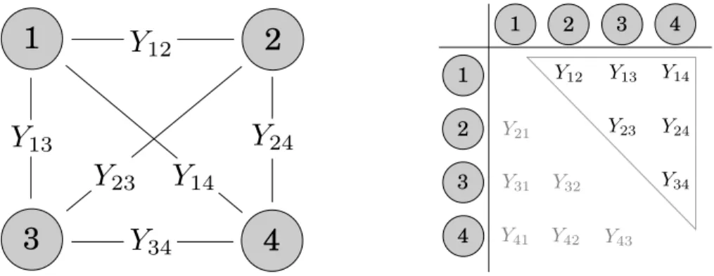
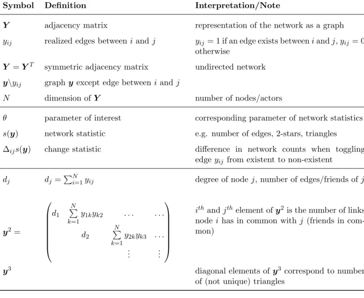
The following notation and terms will be used in this thesis. We focus on modeling network data consisting of N nodes (also called actors or vertices) and edges (also called ties or relationships). Edges are random variables and potential links between a fixed set of nodes. The mathematical graph representation is used to represent a binary network. LetY ∈ {0,1}N×N denote the adjacency matrix of a network withN nodes and
Yij =
(
1, if an edge exists betweeniand j
0, otherwise,
with i, j ∈ {1, . . . , N}. Note that in most approaches and applications self-loops are excluded, i.e.,
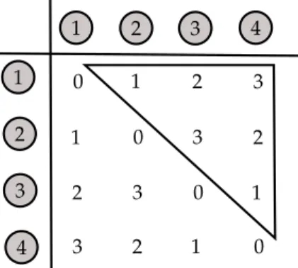
Yii = 0 ∀ i, thus no ties from a node to itself are allowed. In general networks are subdivided in directed and nondirected (also called undirected) graphs, the latter results in symmetric adjacency matrices where Yij = Yji. Figure 1.1 visualizes an undirected toy network of four nodes and all possible tie connections (left panel). The right panel shows the corresponding adjacency matrix, where
Y12 = Y21 etc., which means that this is an undirected network. Classical examples of undirected
1
2
3
4
1 2 3 4 1 2 3 4Figure 1.1: Nondirected network with four nodes and possible edges (left panel), and the corresponding adja-cency matrix (right panel).
networks are friendships or collaborations where people form relationships, however, objects can also be represented by nodes. Email or traffic flows of computer networks usually result in directed graphs.
Note that the random variableY is capitalized, while the observed or realized network is denoted by the corresponding lower case latter (y). There are also extensions where valued ties are considered, however, in this work we focus on binary ties as is defined above. Table A.1 in the Appendix gives a short overview of the notation used here.
So far, the notation considers static networks that do not evolve over time. In the second contributing article of this thesis, we propose an approach for a smooth dynamic network model. Therefore, we extend the notation to time dependent networks. To be specific, letYij(t) be an entry of a matrix valued Poisson processY(t)∈RN×N with cumulated number of events of actoriandj at timetwith
N actors and i, j = 1, . . . , N. We only observe the process at discrete time points t(1), t(2), . . . , t(m)
and defineYij,d=Yij(t(d)) for the evolving process.
1.3
Data examples
This thesis deals with two different data sets: (1) a snapshot of Facebook friendships and (2) patent collaborations evolving over the timespan of 14 years. This section briefly summarizes the most important attributes of these data examples.
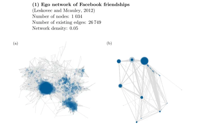
(1) Ego network of Facebook friendships
(Leskovec and Mcauley, 2012) Number of nodes: 1 034
Number of existing edges: 26 749 Network density: 0.05
(a) (b)
Figure 1.2: Facebook network using the force-directed layout algorithm by Fruchterman and Reingold (1991) (a) and the ‘Distributed recursive (Graph) Layout’ (b).
In the first article we apply our estimation approach to a subset of Facebook data collected from a survey by Leskovec and Mcauley (2012). We use a subset of one out of ten ego networks available from the Standford Large Dataset Collection (see Leskovec and Krevl, 2014). An ego network consists of a focal node (“ego”) and all directly connected nodes including their ties to each other. In the following we exclude the ego node. The remaining network is shown in Figure 1.2 using two different layout algorithms, one is based on the force-directed algorithm by Fruchterman and Reingold (1991), and the other uses the ‘Distributed recursive Layout’ (DrL) (see Martin et al., 2008), which focuses on large graphs.
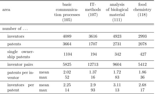
In the second article the model approach is applied to a large dynamic network of patent collaborations of inventors with at least one inventor residing in Germany. The patents were submitted to the European Patent Office (EPO) and the German Patent and Trademark Office (Deutsches Patent-und Markenamt, DPMA). The data contain the submission date on a daily basis, an index list of involved inventors, and the technological area in which the patent is submitted. Moreover, we have information about the geographic coordinates of the inventors at the time of submission.
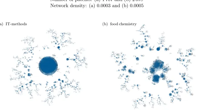
(2) Patent collaboration network of inventors
European Patent Office and German Patent & Trademark Office Number of inventors: (a) 3 616 and (b) 2 993
Number of patents: (a) 1 707 and (b) 2 078 Network density: (a) 0.0003 and (b) 0.0005
(a) IT-methods (b) food chemistry
Figure 1.3: Visualization of two inventor networks aggregated over time for two technological areas. Vertex size represents nodal degree.
We focus on four technological areas and include only inventors with at least one joint patent over the time period from 2000 till the end of 2013. Let the inventors be the nodes and the joint patents the edges of our network graph.
Figure 1.3 shows two of these four networks, which are aggregated over time. Note that these networks contain loops, which belong to single invented patents of inventors with at least one joint patent. Moreover, these illustrations contain multiple edges because the same inventor pair is able to submit several joint patents at different times. Furthermore, we see a few clusters referring to patents with a higher number of inventors or inventors with a lot of joint patents. The densities of the two networks per time point vary between 0 and 0.0005.
1.4
Exponential random graph models
1.4.1 Introduction and basic concepts
The reason for finding a statistical model for network data and not just using descriptive techniques like calculating the density or centrality measurements is easy to understand. A statistical model is able to control for both, a repeating pattern in the process of forming and dissolving ties and for unstructured variability. We consider the observed network to be a realization of a set of networks with similar patterns. Our aim is to extract the most important features of the process that generated the observed network. Inference allows us to assess uncertainty, estimate the amount of contribution of multiple mechanisms, and combine network structure with attributes.
The class of Exponential Random Graph Models (ERGMs) is a promising model class for capturing structural tendencies of social networks. These statistical models are able to include complicated dependence structures due to a variety of network statistics. We can think of network statistics as summary measures or equivalent to covariables in regression models. Some of the most important structures in undirected social networks are homophily and transitivity. Homophily expresses the tendency that actors with similar properties are more likely to form a relationship. The well known statement “friends of my friends are my friends” denotes a greater propensity to make friends between two unconnected actors if there are already common friends and leads to transitivity. Frank (1991) as well as Wasserman and Pattison (1996) propose a model of the form suggested by Frank and Strauss (1986), which includes arbitrary statistics for directed and undirected graphs. This leads to the definition of exponential random graph models, where we assumeY to be random with a probability function
Pθ(Y =y) =
exp (θ0s(y))
κ(θ) y∈ Y, (1.1)
with θ = (θ1, . . . , θp) being the parameter vector of interest and s(·) = (s1(·), . . . , sp(·)) the corre-sponding vector of network statistics. We denote the adjacency matrix of a graph withyand introduce the normalizing constantκ(θ), which is necessary for a probability distribution. This constant
κ(θ) =X y∈Y
is a sum over all possible networks and therefore unfeasible to calculate for large networks. If we con-sider for example undirected graphs on N nodes, the sample space consists of 2(N2) elements.
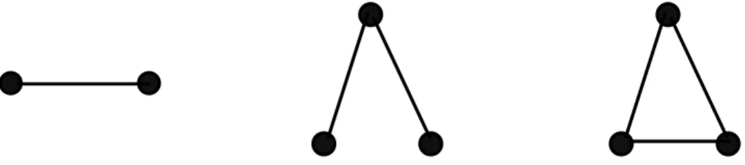
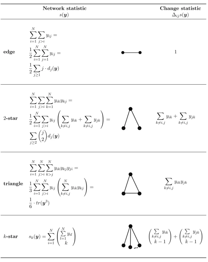
There-fore, estimation requires simulation based methods using numerically demanding routines (Markov chain Monte Carlo) (for more details see Section 1.4.3). In principle, we can include any network configuration ins(·), whereby classical structural network statistics for undirected graphs are counts of edges, 2-stars, or triangles that are visualized in Figure 1.4. An overview of the definitions of these statistics can be found in Table A.2. The 2-star statistic can be written as the sum of the upper
Figure 1.4: Examples of network statistics: edge, 2-star (or 2-path), and triangle.
triangle matrix of the squared adjacency
s2(y) = N X i=1 X j>i N X k=1 yikykj.
The{i, j}-th element of the squared adjacency matrixy2corresponds to the number of links that node
iand nodej have in common, in other words, the number of common friends. Another interpretation would be that the edge and 2-star statistic is the mean and variance of the degree distribution:
s1(y) = 1 2 X j≥1 j·dj(y) and s2(y) = X j≥2 j 2 dj(y),
where dj is the number of nodes of degree j. Therefore, the edge parameter models the average number of edges per node and the 2-star parameter captures the variation in the number of edges of each node. The triangle statistic is defined as
s3(y) = N X i=1 X j>i X k>j yikykjyji = 1 6·tr(y 3),
wherey3 corresponds to the number of paths of length three and tr(·) denotes the trace of a matrix. The triangle effect captures network clustering, like the phenomenon of “a friend of a friend is a friend”.
In recent years extensions of these simple summary statistics have become popular. New specifications like geometrically weighted degree (GWD), alternating k-star, and alternating k-triangle statistics were developed by Snijders et al. (2006) and are introduced in more detail in Section 1.4.4.
It is also possible to include actor attributes expressing for example the already mentioned homophily effect. We can allows(y) to incorporate information of exogenous covariates on nodes and edges that are independent of the actual state of the edges. Moreover, network statistics are able to combine exogenous and structural covariates. For instance, if we consider a friendship network one could consider adding the number of common friends of the same age range, which is a combination of the graph itself and the nodal covariate age.
Most estimation routines of ERGMs are based on simulations using Markov Chain Monte Carlo (MCMC) methods. Therefore, a short note on the conditional form of the ERGM in (1.1) being expressed through logit Pθ Yij = 1 Yhk=yhk, ∀(h, k)6= (i, j) =θ0∆ijs(y) (1.3)
is helpful. This conditional distribution, given the rest of the network for each dyad (pair of tie variables of two nodes), allows interpretation based on a single edge between i and j. ∆ijs(y) is defined as the change in the network statistic vector, which indicates the difference in network counts (e.g. edges, 2-stars, triangles), where a tie is present at (i, j) or not, given the rest of the network. These so-called change statistics are defined by
∆ijs(y) =s(y\yij, yij =yji= 1)−s(y\yij, yij =yji = 0),
that is, we toggle the edge yij between nodes i and j from present to absent. We denote the rest of the graph, except for the tie yij as y\yij. The change statistics of the network configurations in Figure 1.4 are easy to indicate and interpret. For example, we consider a model with these three network statistics, hence the change in the 2-star denoted by Pk6=i,jyik+Pk6=i,jyjk, expresses the sum of friends ofiand j, given the rest of the network. The corresponding parameter indicates the linear effect of one additional friend of i or j on the log-odds assuming all other covariates remain the same. A similar interpretation follows from the triangle change specified throughPk6=i,jyikyjk, which indicates the number of friends thati and j have in common. The parameter of the triangle statistic expresses the effect of an additional joint friend, given the rest stays the same.
A second important part, beside the choice of network statistics, is the assumed dependence structure. These two steps go hand in hand as the dependence assumptions imply a particular model class, which corresponds to certain parameter configurations. This is explained in the next Section 1.4.2 in more detail. For a brief introduction and more details to ERGMs we refer to Lusher et al. (2013), Robins et al. (2007b) and Snijders et al. (2006).
1.4.2 Dependence assumptions
A fundamental concept in ERGMs is the assumption of dependence between observations. Different forms of dependence have been proposed over the last decades. In the following, we give a short overview of the most important concepts. The simplest form of dependence leads to the Bernoulli graphs of Erd˝os and R´enyi (1959). Later, Holland and Leinhardt (1981) introduced the p1 model
class, which is based on the dyadic independence assumption for directed graphs. These simple but restrictive assumptions have been extended, leading to the exponential random graph model, which has also been called p∗ model class by Frank and Strauss (1986). These authors introduced Markov dependence, which was further developed by Pattison and Robins (2002) to realization-dependent models, which assume that two tie variables are even conditionally dependent without sharing a node but with a third tie variable being present. In the class of Markov models one can distinguish between nondirected Markov random graphs, Markov models with new specifications of alternating star parameters, and directed Markov graphs. Our work is based on the first subgroup, whereby we describe the nondirected Markov random graph model in more detail below. For more details see Lusher et al. (2013).
Bernoulli assumption
In a Bernoulli graph all tie variables are assumed to be independent. The (log-) probability of a Bernoulli graph is proportional to the density, which is the weighted sum of the number of edges. The logit of the conditional probability of a tie in a Bernoulli model is given by the edge parameter. To model the adjacency matrixY of a network, only the edge parameter, the corresponding statistic for the number of edges, and the normalizing constant are needed.
Dyad-independent assumption (for directed graphs)
A graph fulfils the dyad-independent assumption if the so-called dyads are independent of each other, which allows the tie from itoj to be independent of the tie fromj to i. This assumption allows for tendencies toward reciprocation.
Markov dependence assumption
Two tie variables are assumed to be dependent, given the rest of the graph, if they share a node. The (log-) probability of a Markov random graph can be calculated – except of a constant – from different network statistics like edges, stars, and triangles.
Nondirected Markov random graph model
Nondirected Markov random graph models are based on the Markov dependence assumption, where two tie variables are assumed to be dependent, given the rest of the graph, if they share a node. With this assumption, a full Markov model only depends on the following statistics: the number of edges, the number of k-stars, and the number of triangles. These configurations are nested because higher-order statistics contain lower-order statistics. For example a triangle consists of three 2-stars and three edges. This characteristic allows statistical inference about the necessity of higher-order given lower-order configurations.
For this work, an important nested subset of the full Markov model is the triad model of Frank and Strauss (1986). This model includes the number of edges, 2-stars, and triangles, which captures both, the mean and variance of the degree distribution, and transitivity and clustering.
A limitation of these nondirected Markov random graph models is that these statistics alone do not fit well to social network data, for which social circuit models were developed. The problem with
models based on the Markov dependence assumption is that complex social structures in real data cannot be captured with these simple statistics.
1.4.3 Estimation of exponential random graph models
“Far better an approximate answer to the ‘right’ question, which is often vague, than an ‘exact’ answer to the wrong question, which can always be made precise.”
– John W. Tukey (Tukey, 1962) For some years after Frank and Strauss (1986) published their seminal paper on exponential random graph models, the estimation of social networks was restricted to pseudo-likelihood estimation ignoring the dependence structure. Later, Geyer and Thompson (1992) suggested a stochastic algorithm to approximate the maximum likelihood estimate in equation (1.1). Since then a variety of estimation routines were developed. Snijders (2002), for instance, proposed a stochastic approximation algorithm based on an approach of Robbins and Monro (1951), or Bayesian inference based on prior distributions for the unknown parameters were introduced. In the following we focus on the most important concepts and refer the reader to additional literature (e.g. Lusher et al., 2013; Snijders, 2002; Strauss and Ikeda, 1990; Van Duijn et al., 2009) for approaches that are not detailed here.
This section ends with an introduction to network simulation because most of the estimation ap-proaches require simulation procedures. After fitting a model, goodness-of-fit statistics or the ex-amination of graph features are based on making draws from the distribution of graphs. Therefore, one contributing article of this thesis focuses on parallel sampling in Markov graphs to accelerate computation.
Pseudo-likelihood estimation
The first paper of exponential random graph models of Frank and Strauss (1986) already pointed out the difficulties of the parameter estimation in ERGMs (1.1). Strauss and Ikeda (1990) came up with an idea based on a method of Besag (1974) for spatial models that ignores the assumed dependence structure. This pseudo-likelihood approach approximates the maximum likelihood estimation and is computationally equivalent to a logistic regression. For undirected networks, the upper triangle entries of the adjacency matrix correspond to the binary response and the change statistics of equation (1.3) to the predictor vector. The pseudo-log-likelihood for undirected graphs is defined as
l(θ) = N X i=1 X j>i lnPθ Yij =yij Yhk=yhk, ∀(h, k)6= (i, j) , (1.4)
where for each potential edge in the adjacency matrix the probability, conditioned on the rest of the graph, is summed up. Finding the maximum for equation (1.4) is straightforward, though this pseudo-likelihood estimator (MPLE) is often less efficient and biased (see Van Duijn et al., 2009). Alternatives have been suggested to correct or to avoid this bias in general.
Maximum likelihood estimation: Geyer-Thompson approach
Geyer and Thompson (1992) suggested an algorithm based on the maximum likelihood principle saying that the maximum likelihood estimator (MLE) for a given model and observed data is the value that makes obtaining the observed data most likely. The method uses Markov chain Monte Carlo approximations of the likelihood function (1.1) and was first applied to ERGMs by Handcock (2003a) and extended to curved ERGMs by Hunter and Handcock (2006). This algorithm relies on simulations in order to maximize the ratio of two likelihoods instead of directly evaluating the log-likelihood
l(θ) =θ0s(y)−log (κ(θ)), (1.5)
with its intractable normalizing constant. Let θ˜be an arbitrarily fixed parameter, we can rewrite expression (1.5) as
l(θ)−l(θ˜) = (θ−θ˜)0s(y)−log κ(θ)
κ(θ˜)
!
, (1.6)
where the ratio of normalizing constants can be approximated by the sample mean. To be more specific, we can reformulate the ratio
κ(θ) κ(θ˜) = X y∈Y expθ−θ˜0s(y) expθ˜0s(y) κ(θ˜) =Eθ˜ expθ−θ˜0s(Y) , (1.7)
with the definition of expectation and formula (1.2). Hence, we approximate the expectation in (1.7) through the sample mean
κ(θ) κ(θ˜) ≈ 1 M M X m=1 expθ−θ˜0sY(m) (1.8)
by exploiting the law of large numbers and replacing the ratio of constants in equation (1.6). To do this, we draw a random sample Y(1), . . . ,Y(M) from the distribution defined byθ˜, which we obtain by Markov chain Monte Carlo simulations described at the end of this section.
A crucial point in the algorithm is that the parameter θ˜ has to be close to the true maximum likelihood estimator, in other words,s(y) lies in the relative interior of the convex hull on the sample of statistics s Y(1), . . . s Y(M) (Hummel et al., 2012). A good first choice to start with is the MPLE, but typically the algorithm has to be restarted several times (see e.g. the implementation in Handcock et al., 2017). Hummel et al. (2012) developed the “stepping” algorithm to systematically move closer to the true estimator by defining pseudo-observations, which guarantee to stay in the convex hull of the sample. Combining this and a log-normal approximation maximum likelihood estimation procedures can be carried out, which leads to an improved estimation (see Hummel et al., 2012).
Stochastic approximation: Robbins-Monro algorithm
An alternative approach using maximum likelihood estimation for finding unknown parameters has been proposed by Snijders (2002). This version of the Robbins and Monro (1951) algorithm works without large samples of graphs or good starting parameters. The main aim of this stochastic ap-proximation algorithm is to solve the moment equation. Finding the MLE or solving the moment equation
Eθ(s(Y)) =s(y) (1.9)
is equivalent because equation (1.9) is satisfied if and only if ˆθ is the maximum likelihood estimator ofθ. This iterative procedure updates the parameter vector θ(m) in each iterationm through
θ(m+1) =θ(m)−arD0−1
sy(m)−s(y), (1.10)
a Newton-Raphson-type equation, whereD0 denotes a scaling matrix from an initial phase. In each update step, one sampled graph s y(m) from the ERGM with parameter θ(m) based on MCMC methods is generated. The factorar guarantees a decreasing weight of the changes with increasing number of iterationsm. For more details or extensions see, e.g., Snijders (2002), Lusher et al. (2013) and Okabayashi et al. (2012).
Simulation methods
A very important part in the inference of exponential random graph models in (1.1) is to sample graphs from a target distribution based on Markov chain Monte Carlo methods. Most of these models are intractable because of their normalizing constant. Nevertheless, evaluating the conditional probability of an edge, assuming the rest remains the same, is straightforward because the constant cancels out. Therefore, making draws from an ERGM is often possible and not computational expensive. The basic idea of a Monte Carlo procedure is to generate a sequence ofLgraphs Y(0),Y(1), . . . ,Y(l), . . . ,Y(L) by successively updating a tie variable until theLth network, with large enough L, results in a draw from the target distribution of our ERGM. There are two famous algorithms that are mostly used to simulate networks: a Metropolis-Hastings sampling algorithm (Metropolis et al., 1953; Hastings, 1970) or a Gibbs sampler (Geman and Geman, 1987), which is a special case of the first and simulates the edges based on the logit model resulting from (1.1). Note that in most cases Metropolis-Hastings algorithms converge more efficiently because the changes in the adjacency matrix are more frequent. In the following we focus on the Metropolis-Hastings algorithm because the first contributing article of this thesis is based on this method.
We start the Metropolis-Hastings sampler (see also Lusher et al., 2013; Hunter et al., 2008b) with an empty or the observed networkY(0) and sequentially update edges creating L networks. In each iterationlforl= 1, . . . , L, we randomly choose one dyadyij(l−1) for updating. The proposed network
Y∗ is equal to the current graph Y(l−1) but one node pair is toggled from y(l−1)
ij to 1−y
(l−1)
ij . We
add or remove this tie with a certain acceptance probability min 1, Pθ(Y∗) Pθ(Y(l−1)) , (1.11)
with Pθ(Y) being the target distribution. This so-called “Hastings ratio” denotes the ratio of how much more likely the new proposed graph is compared to the old one. If the new proposal has a higher probability, we accept the toggle, if it has a lower probability, we accept the change with a certain probability depending on the difference. If the change is accepted, we set Y(l) =Y∗, otherwise, we set Y(l) =Y(l−1). After that we start again by choosing an edge to toggle till our graph is a draw from the target distribution.
Note that no normalizing constant is needed because the Hastings ratio (1.11) can be expressed as log P θ(Y∗) Pθ(Y(l−1)) = lognP(Yij = 1−yij(l−1)|Y\Yij =yij(l−1)) o =θ0∆ijs(y), (1.12)
where only the differences in the statistics that result in changingyij(l−1) to 1−yij(l−1) are needed. We have already encountered this closed form in the section on conditional distributions of ERGMs (1.3), where we called ∆ijs(y) the change statistic for adding an absent tie. Here in equation (1.12), we define the change statistics as the differences in the statistics that result in toggling a tie from zero to one or from one to zero.
The fundamental principle behind Markov chain Monte Carlo simulations is that once the sampler settles into the target distribution – after a certain number of iterations (“burn-in”) – the next graphs also derive from the ERGM. Therefore, the simulation chain just has to be started once. After a reasonable number of burn-in iterations the first network is simulated and after further iterations the Markov chain has ‘forgotten’ the last state and produces additional networks from this given distribution. These so-called “thinning” steps guarantee independent draws. If the burn-in is large enough, the algorithm is independent of the starting network.
Since inference or goodness-of-fit algorithms require us to simulate a large number of networks by generating a sequence of L graphs each, it is important to use an efficient algorithm. A good choice for speeding up the sampling algorithm is the “TNT” (tie-no tie) sampler proposed by Morris et al. (2008). The TNT sampler modifies the Metropolis-Hastings MCMC routine by not selecting the dyads to toggle randomly but with certain probabilities depending on the actual state of yij. In practice, most networks are sparse and therefore, for random samplers the probability to select an empty dyad and propose a change, which is rejected, is very high. In such cases the Markov chain often stays longer in the same state. To avoid this, the TNT sampler chooses present and absent edges with a probability of 0.5 each, which leads to a faster convergence of the Markov chain. Further modifications of the simulation procedures to improve convergence of the Markov chains, computation time, and properties of the simulated networks exist in the literature. An idea of Snijders (2002) is to update multiple edges e.g. in form of triples or other natural groups of entries
in the adjacency matrix at once. The decision process follows the same scheme as described above but for multiple edges simultaneously. If a change is accepted, all dyads in the set are updated. The groupwise probabilities are defined analogously but for the set of all possible outcomes for the elements.
Snijders (2002) proposed as well to include “big updates” in the switching process to avoid convergence problems. The idea is to update a bigger set of edges like rows or columns based on the concept of the cluster-flipping algorithms for the Ising model (see Newman and Barkema, 1999). To extend this, the set of edges consists of the complete network graph and results in its inversion. Nevertheless, such an inversion step only occurs with a certain but small probability instead of a ‘normal’ step. Referring to the quote of Tukey (1962) at the beginning, it is sometimes better to meet the challenges of using a maximum likelihood approach by approximating it and getting an answer to the ‘right’ question, than using the simple pseudo-likelihood estimation and getting an ‘exact’ answer to the wrong question.
1.4.4 Degeneracy problems
The estimation routines of exponential random graph models mentioned above that are used to solve the problem of the intractable normalization constant, all rely on simulation approaches based on Markov chain Monte Carlo methods. Thus, e.g. Snijders (2002), Snijders et al. (2006), Handcock (2003a) or Handcock (2003b) address the problem of model degeneracy, which is related to these procedures. The stationary distribution is termed degenerated if the probability distribution is con-centrated on a small subset of sample space. Handcock (2003a) defines the term near-degeneracy as a distribution assigning disproportionate probability mass to a small outcome space, where the parameters lie on the boundary of the convex hull. Especially network models with simple statistics like 2-stars, k-stars, and triangles typically suffer from (near) degeneracy problems because of the so-called avalanche effect of the change statistics, where positive parameters result in a large increase of the change statistics and always get larger (see Snijders et al., 2006). Schweinberger (2011) explores different settings of ERGMs and discovers that these models favour graphs with a transition from low-density to high-density graphs, making inference unstable and leading to convergence problems of the algorithms.
Snijders et al. (2006), Robins et al. (2007a) or Wang et al. (2013) propose ideas avoiding this avalanche effect by using configurations like the alternating k-stars or k-triangles leading to the social circuit models. Accordingly, Snijders et al. (2006) define alternatingk-stars as
u(λs)(y) =S2− S3 λ + S4 λ2 −. . .+ (−1) N−3SN−1 λN−3 = NX−1 k=2 (−1)k Sk λk−2, where Sk(y) = PNi=1 yik+
for k ≥2 is the number of k-stars and yi+ is the degree of node i. The alternating sign of the weights balances adjacentk-star counts and decreases problems of degeneracy. Modeling transitivity by using triangle counts and triangles of higher order often results in degenerated
models. Therefore, Snijders et al. (2006) defined – similar to the alternatingk-stars – the alternating k-triangles as u(λt)(y) = 3T1− T2 λ + T3 λ2 −. . .+ (−1) N−3TN−2 λN−3, where Tk= N X i=1 N X j>i yij P h6=i,jyihyhj k
is the number of k-triangles fork≥2 and
T1 = 1 3 N X i=1 N X j>i yij X h6=i,j yihyhj
is the number of 1-triangles. Note that Ph6=i,jyihyhj is the change statistic of the triangle counts. These ideas are aimed at reducing the weight of the linear effect of the statistics. The same motivation is used in Thiemichen and Kauermann (2017) by proposing a non-parametric ERGM or in the first contributing publication (Bauer et al., 2019) by using a logarithmic transformation of the change statistics that stabilizes the estimation but keeps the interpretability of the parameters.
1.4.5 Challenges and solutions in speeding up computation time
A crucial aspect for estimating large networks is having a reasonable computation time. Several proposals to speed up the time consuming simulation methods have been made by e.g. Morris et al. (2008), who suggested the “TNT” sampler or Snijders (2002), who described a version to update multiple edges simultaneously. These modifications are explained in more detail at the end of Section 1.4.3. The TNT sampler aims to converge more quickly to the target distribution, but is only useful for quite sparse or dense networks, which can be seen in the traceplots in the first contributing publication.
An obvious idea to reduce computation time is to adopt parallel computing, however, parallelization of networks is not straightforward due to the dependent data structure of networks. Handcock et al. (2017) have implemented an option of parallelization in the estimation routines of theRpackageergm, which is able to exploit multiple CPUs, CPU cores or computing clusters. However, this option starts multiple Markov chains simultaneously, leading to an increasing memory and a lower improvement of computation time. Further details and comparisons are evaluated in the first contributing article in Chapter 2, where a different approach of simulating networks in parallel is discussed.
One key rule for parallel computing is that communication between workers (also called threads) costs a lot of time. Therefore, the aim is always to keep the communication to a minimum and to maximize the size of work in each divided step (see Schmidberger et al., 2009). This key rule led us to our first idea, which we call the “block-parallel” algorithm. This algorithm is also based on the Markovian independence assumption to draw independent node pairs in a network, which is described in more detail in Chapter 2. Summing up, we need to construct a way to draw independent node pairs, thus node pairs, which do not share a node. The first way of making use of the Markovian structure in
the simulation step is the one mentioned in the first contributing publication of this thesis where nodes are shuffled randomly, paired and sent to different computing cores as independent tasks. The second possibility is constructing independent node pairs from a symmetric Latin square with a unique diagonal (see e.g. Andersen and Hilton, 1980). Figure 1.5 shows such a Latin square decomposition for a four node example. The adjacency matrix for undirected graphs is symmetric, which means
1 2 3 4 1 2 0 3 0 0 0 1 1 1 2 2 2 3 3 3 1 2 3 4
Figure 1.5: Visualization of a symmetric Latin square with a unique diagonal for a four node example.
it is sufficient to only consider the upper triangle. The numbers in the upper triangle correspond to the simulation steps in the parallel Metropolis-Hastings sampler. In the first simulation step, the node pairs (1,2) and (3,4) can be simulated simultaneously. In the second step, we simulate the pairs (1,3) and (2,4) in parallel, and in the third step (1,4) and (2,3). This procedure is scalable to larger networks with an increasing number of computing nodes. AssumingN/2 computing cores, we can complete a Metropolis-Hastings loop inN−1 steps. Therefore, the computing time for network simulation increases just linearly with the number of nodes in the network (N), if sufficient computing cores are available. Obviously, when the number of nodes in a network is large, we may not have access to N/2 computing cores. It is also likely that the communication task between the cores is getting too demanding and devours the computational gains.
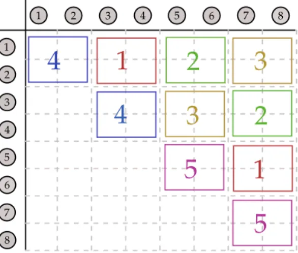
One solution for this kind of problem is a blockwise decomposition of the adjacency matrix by extend-ing the conditional independence ideas from above. In this case, not only sextend-ingle edges are simulated on the cores, but blocks of independent pairs of edges are simulated. This speeds up the computa-tion through the faster pre-processing as well as through saving time because of less communicacomputa-tion between the cores. We therefore select submatrices of the adjacency matrix. This approach is also advisable if the number of nodes in the network is large and only a fixed number of cores is available. Figure 1.6 visualizes the idea of grouping a network withN = 8 nodes into independent blocks of node pairs. The block number indicates the step number. Blocks with the same number can be simulated simultaneously. In this example, two computing cores complete one Metropolis-Hastings loop in five rounds as the diagonal elements of the Latin square have to be considered at least halfway. In the first simulation step, we consider the edgesY13, Y14, Y23,and Y24 sequentially on one core and at the same time the edges Y57, Y58, Y67, and Y68 on the other core, in other words, in parallel. These are
1 2 3 4 1 2 3 4 5 8 7 6 5 8 7 6
1
4
4
5
5
3
3
1
2
2
Figure 1.6: Visualization of a blockwise decomposition of an eight node example with the help of a symmetric Latin square.
the submatrices with entry one in the blockwise Latin square in Figure 1.6. The other steps follow the same scheme.
A comparison of the performance between the single entry choice of edges (called “parallel”) and blockwise decomposition is shown in Figure 1.7, where three networks are simulated on eight cores for different numbers of nodes. Obviously, a reduction of computing time is achieved for the
block-● ● ● ● ● ● ● ● ● ● ● ● ● ● ● ● ● ● ● ● ● ● ● ● ● ● ● ● ● ● ● ● block−parallel parallel 200 1200 2200 200 1200 2200 0 5 10 15 number of nodes (N) time [seconds]
Figure 1.7: Performance of block-parallel and parallel algorithm for different network dimensions. They-axis shows time in seconds to simulate three networks on eight cores.
parallel algorithm especially for large networks with N = 2200 nodes. The main reasons for this are the reduction of communication costs and the load balancing as well as the optimization of data locality issues.
1.4.6 Further restraints and open questions
The field of statistical network analysis is still not completely explored and a lot of research can be done to improve estimation algorithms, or handle different kinds of networks like ones with valued edges (e.g. Krivitsky, 2012; Desmarais and Cranmer, 2012a), missing data (e.g. Handcock and Gile, 2010; Koskinen et al., 2010), and nodal heterogeneity (e.g. Krivitsky et al., 2009; Thiemichen et al., 2016).
Even though estimation methods that try to find the (approximate) maximum likelihood estimator exist, one has to keep in mind that the Markov chains only run a finite time whereas the optimal result would be obtained after an infinite number of steps. Moreover, existing goodness-of-fit routines rely on simulating graphs from the fitted model and compare their statistics graphically to the observed analogues (cf. Hunter et al., 2008a). However, it remains unclear if the simulated networks come from the ‘true’ distribution or only resemble the network statistics. A surprising fact was found by Handcock (2003a), who fits an ERGM and then compares a large number of simulated networks to the observed one. The simulated networks differ a lot due to the extremely high number of possibilities. The maximum likelihood estimator of a parameter is the value that makes observing a given network most likely, though in most cases the probability in comparison to all possible networks is not high enough.
1.5
Dynamic network models
The second contributing article of this thesis suggests a smooth dynamic network model for patent collaboration data. This model focuses on a profile likelihood approach to model time-stamped event data based on a multivariate counting process. First, an overview of existing dynamic models for network data is given, which is followed by a short introduction of counting processes and the profile likelihood approach based on the Cox model (Cox, 1972). We further explore similarities of the Cox proportional hazards and (additive) Poisson model. We extend this analogy to additive Poisson models because we propose in our article a semiparametric approach including covariates more flexible by penalized smoothing techniques.
1.5.1 Outline
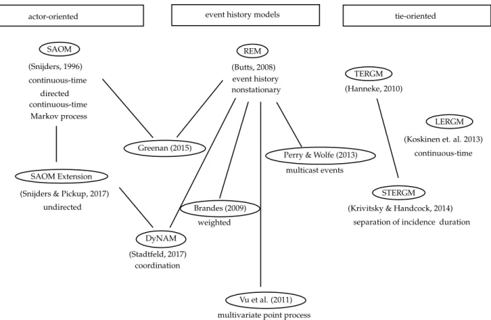
Originally, the analysis for dynamic network data focused on collapsed panel data (e.g. Hanneke et al., 2010) or small networks with only a few observation times and a few hundreds of nodes (Snijders, 2001, 2005). On the one hand, most of the time data collection depends on discrete and manually gathered information, on the other hand, methods for large and time-stamped data are lacking. In general, models for dynamic network data can be divided into three, overlapping and not encompassing, strands: actor-oriented, tie-oriented, and models based on event history (see Figure 1.8 for an overview). The most known models of these strands are the Stochastic Actor-Oriented Model (SAOM) of Snijders (2001), tie-oriented models like the extensions of the Exponential Random Graph Model (ERGM) to longitudinal (LERGM; Koskinen and Snijders, 2013) or temporal (TERGM;
Hanneke et al., 2010) network models, and the Relational Event Model (REM) of Butts (2008). The main differences are different model assumptions that decide about the interpretation of the estimates and the conclusions, which can be drawn. In comparison to SAOMs, which are actor-oriented, ERGMs are global models and focus on the importance of tie structures. Furthermore, the treatment of time differs for these models whereby SAOM and LERGM follow a continuous-time and TERGM follows a discrete-time process. A crucial difference between tie-oriented models and event history models is that the former models a stationary distribution whereas the latter models the changes between two time points and focuses on the search of driving forces for the network evolution and not on predicting future ties.
actor-oriented event history models tie-oriented
TERGM LERGM SAOM SAOM Extension REM DyNAM Brandes (2009)
Perry & Wolfe (2013) Greenan (2015)
Vu et al. (2011)
STERGM
(Krivitsky & Handcock, 2014) (Hanneke, 2010)
(Koskinen et. al. 2013)
(Stadtfeld, 2017) (Snijders & Pickup, 2017)
undirected continuous-time (Snijders, 1996) continuous-time continuous-time directed Markov process coordination
multivariate point process multicast events
weighted
nonstationary event history
separation of incidence duration (Butts, 2008)
Figure 1.8: Overview of existing dynamic models (not encompassing).
In the following, we introduce the basic concepts of the most important models in dynamic network analysis starting with the first approaches in this field.
Snijders (1996) proposed a model class for longitudinal network data known as stochastic actor-based model (see also Snijders, 2001, 2005; Snijders et al., 2010). SAOMs focus on network dynamics influenced by the change of relations, which are driven by an actor. This actor-oriented perspective has the consequence that tie changes are modeled as results from actions by actors, more precisely, that actors control their outgoing ties. Hence, SAOMs are actor-driven. These decisions are nested
in a Markov process, i.e., for any point of time the present network is not affected by past events, but provides insight into its further development. The models are based on continuous-time Markov chain models although the networks are observed at discrete times with a finite number of observation waves. The network evolution or dissolution process is divided into two parts. The first part determines the waiting time until a change in the network is made by one actor and is modeled by optimizing a ‘rate function’, which contains information about the general affinity of changing ties of each actor. The second part is called ‘objective function’ and represents the utility of certain possible tie changes for an arbitrary actor. This function determines the preferred network over the set of all possible ones and is based on a multinomial logit model. Both sub-processes depend on exogenous covariates, endogenous network effects, or effects derived from network positions. The estimation is done using the method of moments approach with stochastic approximation by Robbins and Monro (1951). Snijders and Pickup (2017) extent the latter model for nondirected ties by using a two-step process of opportunity and choice. The two-sided choice resulting from undirected relations is decomposed into a timing or opportunity process with one- or two-sided initiatives and a choice process. The latter process uses one of three opportunities: agreement about a tie between two actors, one actor decides alone about a tie, or the decision is based on a combined objective function. Depending on different assumptions regarding various applications, one of these six combinations is selected as modeling approach. An early attempt extending the exponential random graph model to dynamic network data settings has been proposed by Robins and Pattison (2001) and was further explored by Hanneke et al. (2010). The idea of Robins and Pattison (2001) is to use a Markov random graph approach for temporal evolution of social networks by generalizing the process to changes of discrete time points. Hanneke et al. (2010) called this extension Temporal Exponential Random Graph Model (TERGM) and added algorithmic and inferential developments like hypothesis tests, more flexible parametrization, and explorations of statistical properties. A major point of these discrete temporal models is the Markov dependence assumption over time. At each time t a network Yt is assumed to be independent of
Y1, . . . ,Yt−2 givenYt−1. More generally, a TERGM that incorporates dependencies ofK previously observed networks is denoted by
Pθ(Yt|Yt−K, . . . ,Yt−1,θ) =
exp{θ0s(Yt,Yt−1, . . . ,Yt−K)}
κ(θ,Yt−K, . . . ,Yt−1) , (1.13) where the choice of K ∈ {0,1, . . . , T −1} needs to be in line with the temporal dependence of network Yt. Estimation of TERGMs can be carried out by maximum likelihood methods using MCMC sampling techniques to approximate the intractable normalizing constant. These estimation approaches resemble the ones used in ERGMs, but have small differences. Like in the time-invariant ERGM, the procedures used are challenging and computationally expensive. Therefore, Desmarais and Cranmer (2012b) suggested a pseudo-likelihood approach with bootstrap confidence intervals to correct the biased uncertainty measurement, which was described by Leifeld et al. (2018) for TERGMs. For detailed information we refer the reader to Hanneke et al. (2010), Leifeld et al. (2018) and Desmarais and Cranmer (2012b).
Krivitsky and Handcock (2014) suggested combining the discrete-time temporal exponential random graph model for network dynamics of Hanneke et al. (2010) with the nonlinear parametrization known as curved ERGMs of Hunter and Handcock (2006). These exponential-family random graph models focus on a separable modeling approach of incidence and duration of ties, calling this model class Separable Temporal ERGM (STERGM). This separate parametrization within a time-step allows for individual interpretation and therefore more flexibility. Within this method, a further distinction between tie formation and dissolution can be explored. In many applications this separation is useful. STERGM can be seen as a subclass of TERGM defined in (1.13) with K= 1.
A natural procedure for modeling event data, including time stamps, is using survival models like the Cox proportional hazards model (Cox, 1972). Generally, events are independent and influenced by exogenous effects. However, when modeling network data, the focus is primarily on potential endogenous factors, which influence network creation and dissolution.
An approach for modeling social behavior dynamically as events or actions is known as the Relational Event Model (REM) suggested by Butts (2008). This framework allows for likelihood-based infer-ence from event data to detect social dependinfer-ence patterns, estimate its strength, evaluate competing settings within this patterns, and allow for non-stationary behavior. The relational event model com-bines network structures with event history models for nondirected and directed ties by exploiting a tie-based approach where potential relations are chosen independently conditioned on the past ac-tions. This framework can include exogenous covariates influencing the future and sufficient statistics capturing the impact of event history. These models aim to combine a theoretical based approach with working inference and estimation for analyzing the process underlying social behavior. The cru-cial point in the REM is the relational event, or action happening at time t∈R when an actor (the “sender”) is pointing towards one “receiver”. It is assumed that the events follow an inhomogeneous Poisson-type process conditioned on the past history and possibly other exogenous covariates. Brandes et al. (2009) developed a framework for modeling dyadic event data of interactions between actors and apply it to political event networks. Similar model specifications can be found in the relational event model of Butts (2008) but with extension to weighted events. Parameter estimation is based on maximum likelihood techniques and assumes an independence between rate and weight parameters. Network statistics to capture reciprocity, structural balance, or activity and popularity effects can be incorporated to detect influences of the network’s past on future events.
Most models in dynamic network analysis focus on directed relations where the actor controls the outgoing ties. In political or social science, however, the question arises how individuals or states in general jointly admit to forming network connections. An example for what Stadtfeld et al. (2017a) call ‘coordination’ networks, are patent collaborations that arise by inventors, who mutually agree to work together and submit joint patents. Stadtfeld et al. (2017a) introduced the Dynamic Network Actor Model (DyNAM) for modeling relational event data of coordination networks. These models consider dependency between observations, are constructed for undirected ties including a two-sided process of building ties, and allow for time-stamped data. Moreover, it is possible to take different mechanisms like tie formation and dissolution, unequal time gaps, and various types of ties into account. DyNAMs aim to investigate dynamic coordination networks with different facets of ties
(weighted, windowed, and signed) and consider internal network structures adjusting for homophily, clustering, or preferential attachment effects. An important question in network science arises when it comes to the decision process of actors formulating their favorable circumstances and preferences given the opportunities. This two-sided process is an agreement of both actors being involved and maybe a more complex dependence structure due to network and temporal dependence (see above two-step process of Snijders and Pickup, 2017). Consider for example that, the data contains the following information:
time inventors sign
month 1 1←→ 2 create
month 2 1←→ 3 create
month 6 2←→ 3 create
The decision process can be influenced by the temporal effect of the first two observations and by the network structure that inventor 1 is involved in both patents of month 1 and 2. Another network dependence assumption might play a role in the third observation because inventor 2 and 3 close a triangle with this patent. Dynamic network actor models are designed for such time-stamped coordination data combining parts of Snijders (1996, 2001) stochastic actor-oriented model and the relational event model of Butts (2008). Stadtfeld et al. (2017a) merge an actor-oriented approach where both actorsiandjselect each other from a set of actors with undirected relations. ‘Still’ actor-oriented, actoriproposes a new tie to j at any time point, andj has to chooseias favored partner. Inspired by Snijders et al. (2010) micro-model in SAOMs for determining the change, DyNAMs are also developed in a continuous-time framework, modeling mutual choices with multinomial probability models. A linear objective function evaluates changes in the process matrix. In order to model the waiting time between tie proposals and realized changes, further steps are included in the model framework. For optimizing the model parameter in the estimation routine, DyNAMs use a maximum likelihood approach. For more details and discussion about the proposed framework see Stadtfeld et al. (2017a,b), Butts (2017), and Snijders (2017).
Vu et al. (2011a) suggested an event history approach focusing on large networks with nodal statistics, which extends earlier work from Butts (2008). This ‘egocentric network model’ of Vu et al. (2011a) uses an efficient optimization algorithm derived from the partial likelihood to estimate nodal pro-cesses based on statistics from network history. Later, Vu et al. (2011b) generalize and extend their approach for dynamic egocentric models (Vu et al., 2011a) to a general continuous-time regression model for longitudinal networks with time-varying network statistics embedded in an Aalen model (Aalen et al., 2008). Furthermore, they unite techniques for a relational framework including a mul-tivariate counting process for edge formation. The focus of their approach is on large networks and efficient inference thereof. In the general framework, Vu et al. (2011b) formulateYij(t) as a counting process, which represents the number of ties from node i toj at time t. In the paper they restrict their model to non-recurrent events and do not take any tie dissolution process into account. The
model considered is based on a multivariate interdependent counting process Y(t) decomposed by the Doob-Meyer theorem (Aalen et al., 2008),
Y(t) =
Z t 0
λ(s) +M(t), (1.14)
with λ(t) denoting the intensity process or hazard rate and M(t) being the martingale noise. The basis for this theory relies on the fact that counting processes are non-decreasing in time and can therefore be regarded as submartingales. The intensity process is modeled in two different ways, a multiplicative Cox or additive Aalen approach, which both take the past of the networks as network statistics into account. λ(t) incorporates linear combinations or time-varying effects of these network statistics. Estimation of the Cox-type model is carried out by exploiting the simplification of just maximizing the so-called partial likelihood instead of the full one. By doing so, the baseline hazard is considered as nuisance parameter. Combining this with the caching method of Vu et al. (2011a) results in an efficient computation for large networks. The estimation of the Aalen model is based on linear regression methods with the possibility to include kernel smoothing techniques for interpretability of time-varying coefficients.
A different approach modeling time-stamped network data for social events is described by De Nooy (2011). Based on a discrete-time event history model, De Nooy (2011) focuses on modeling tie forma-tion, change, or dissolution by combining a multilevel design and time-varying covariates. Network dependencies and endogenous effects are taken into account by applying a multilevel logistic regres-sion analysis approach based on a General Linear (Mixed) Model (GLMM). Therefore, extenregres-sions to a non-dichotomous target variable like a competing risk model in survival analysis is possible. Perry and Wolfe (2013) describe an extension of a multivariate point process approach emphasizing properties of the maximum partial likelihood inference and considering multicast interactions. The authors propose a stratified Cox multiplicative intensity model for directed networks with covariates built from network history. For simplifications, most research excludes simultaneous interactions or uses approximated solutions like the Breslow-Peto correction (Breslow, 1972; Peto, 1972) or the Efron (1977) approximation. Both approaches use a product over the risk terms of the tied events and give a fair approximation of the likelihood function but can in some cases suffer from biased estimations (Scheike and Sun, 2007). Breslow and Peto’s suggestion is easy to compute but the approximation of Efron (1977) is closer to the proper likelihood because weighted risks are used. Perry and Wolfe (2013) evaluate the approximation error between the model that includes multiple receivers explicitly and the one that approximates the partial likelihood. They suggest a bias correction procedure based on parametric bootstrap calculation for that error.
Greenan (2015) transfers the stochastic actor oriented model of Snijders (2001) to dynamic social networks with the evolution of diffusion of innovations by combining the SAOM with a proportional hazards model. The network and diffusion process are combined and considered as dependent on each other, while the adoption times of the latter process follow a Cox regression model (Cox, 1972) with
a hazard function depending on covariates. The network dynamics are modeled via rate function like it is known from the SAOM.
1.5.2 Cox’s regression model and multivariate counting processes for network data
The most famous model class for fitting time-to-event data is known as the Cox proportional hazards model for survival data. Cox (1972) denotes the hazard or intensity rate (for non-recurrent events)
λ(t) = lim ∆t→0
P(t≤T < t+ ∆t|T ≥t)
∆t (1.15)
for the survival time T, describing the risk of having an event at time t, given that no event has occurred until t. The idea is to model the effects of covariates on the hazard rate, rather than the hazard rate itself. For example, does the fact of having joint patents increase or decrease the hazard of submitting new patents? Cox (1972) represents the hazard rate as
λ(t;x) =λ0(t) exp{βTx(t)}, t≥0, (1.16) with covariate vector x(t), which may be time dependent or not and unknown coefficient vector β. The baseline hazardλ0(t) determines the underlying process but is unknown. Due to the individual covariates, the baseline hazard becomes subject-specific. The basic Cox model assumes that all m
event timest(1), . . . , t(m) are distinct, and that the event for subjectdoccurred at timet(d). In order to make inference,β and laterλ, have to be estimated by maximizing
L(β) = m Y d=1 " exp βTx d(t(d)) P d0∈Odexp β Tx d0(t(d)) #δd (1.17)
with respect to β, where t(1), . . . , t(m) are the distinct survival times, Od is the risk set (in our application called ‘option set’) at timet(d)and δdis the event indicator. Later Cox (1975) shows that his suggested likelihood in (1.17) can be derived as the partial likelihood function and that ˆβ is its estimator. For estimating the cumulative hazard Λ(t) =R0tλ(s)ds, Breslow (1972, 1974) proposes the following estimator ˆ Λ(t) = X t(d)≤t δd P d0∈Odexp ˆ βTx d0(t(d)) , (1.18)
based on linear interpolation between survival times. The baseline hazardλ0(t) is commonly treated as nuisance parameter and considered to be a non-negative function with non-zero values over the event time intervals.
Andersen and Gill (1982) and Johansen (1983) extend the model of Cox (1972) captured in equation (1.16) by allowing recurrent events. Johansen (1983) derives a joint likelihood L(β,Λ) from an extended Cox model and demonstrates that the partial likelihood of equation (1.17) derived from the