and the
Theory of Signal Processing with L´
evy Information
by
Xun Yang
Department of Mathematics
Imperial College London
London SW7 2AZ, United Kingdom
and
Shell International Limited
Shell Centre, London SE1 7NA, United Kingdom
Submitted to Imperial College London
for the degree of
Doctor of Philosophy
In mathematical finance, increasing attention is being paid to (a) the construction of explicit models for the flow of market information, and (b) the use of such models as a basis for asset pricing. One notable approach in this spirit is the information-based asset pricing theory of Brody, Hughston and Macrina (BHM), in which so-called information processes are introduced and ingeniously integrated into the general theory of asset pricing. Building on the BHM theory, this thesis presents a number of new developments in this area.
I begin with a brief review of the BHM framework, leading to a discussion of the simplest asset pricing models. Then the first main topic of the thesis, which is based in part on Brody, Hughston & Yang (2013b), is developed, which concerns asset pric-ing with continuous cash flows in the presence of noisy information. In particular, an information-based model for the pricing of storable commodities and associated deriva-tives thereof is introduced. The model employs the concept of market information about future supply and demand as a basis for valuation. Physical ownership of a commod-ity is regarded as providing the beneficiary with a continuous “convenience dividend”, equivalent to a continuous cash flow. The market filtration is assumed to be generated jointly by: (i) an information process concerning the future convenience-dividend flow; and (ii) a convenience-dividend process that provides information about current and past dividend levels. The price of a commodity is given by the risk-neutral expectation of the cumulative future convenience dividends, suitably discounted, conditional on the information provided by the market filtration. In the situation where the convenience dividend is modelled by an Ornstein-Uhlenbeck process, the prices of options on com-modities, both when the underlying is a spot price and when the underlying is a futures price, can be derived in closed form. The dynamical equation of the price process is worked out, leading to an identification of the associated innovations process. The re-sulting model is sufficiently tractable to allow for simulation studies of the rere-sulting commodity price trajectories.
The second main topic of the thesis, which is based in part on Brody, Hughston & Yang (2013a), concerns a generalisation of concept of information process to the situa-tion where the noise is modelled by a general L´evy process. There are many practical circumstances in which signal or noise, or both, exhibit discontinuities. This part of the thesis develops a rather general theory of signal processing involving L´evy noise, with the view to the introduction of a broad and tractable family of information processes suitable for modelling situations involving discontinuous signals, discontinuous noise, and discontinuous information. In this context, each information process is associated with a certain “noise type”, and an information process of a given noise type is dis-tinguished by the message that it carries. More specifically, each information process
is associated in a precise way to a L´evy process, which I call the fiducial process. The fiducial process is the information process that results in the case of a null message, and can be regarded as a “pure noise” process of the given noise type. Information processes can be classified by the characteristics of the associated fiducial processes. To keep the discussion simple, I mainly consider the case where the message is represented by a single random variable. I construct the optimal filter in the form of a map that takes thea priori distribution of the message to ana posteriori distribution that depends on the information made available. A number of examples are presented and worked out in detail. The results vary remarkably in detail and character for the different types of information processes considered, and yet there is an overall unity in the scheme that allows for the construction of numerous explicit and interesting examples. The results presented in the second part of the thesis therefore have the potential to pave the way toward a variety of new applications, including applications to problems in finance.
I, Xun Yang, declare that this thesis, entitled “Information-Based Commodity Pricing and the Theory of Signal Processing with L´evy Information”, and the work presented in it, are my own.
Copyright Declaration
The copyright of this thesis rests with the author and is made available under a Creative Commons Attribution Non-Commercial No Derivatives licence. Researchers are free to copy, distribute or transmit the thesis on the condition that they attribute it, that they do not use it for commercial purposes and that they do not alter, transform or build upon it. For any reuse or redistribution, researchers must make clear to others the licence terms of this work.
In carrying out the work presented in this thesis I have had the opportunity to be supervised both by Professor D. C. Brody and Professor L. P. Hughston, and I would like to express my gratitude to each of them for their help and support. I would also like to thank my examiners, Professor D. Brigo and Professor G. Peskir, for valuable suggestions. This work was carried out under the terms of a sponsored PhD studentship at Imperial College supported in full by Shell International Limited, London. I would like to thank Paul Downie, Nick Wakefield and Andy Longden at Shell for making this opportunity available to me, which has given me an invaluable experience for which I am truly grateful. During the course of my PhD studies I have had the opportunity to meet many people with whom I have had beneficial discussions, and to make many friends, both among staff and students at Imperial College—too many to name—and among colleagues at Shell—again too many to name—but all of whom I would like to thank. I have also benefited from participation in the activities of the wider London mathematical finance community, and from useful feedback concerning presentations of my work by participants at the AMaMeF (Advanced Mathematical Methods in Finance) conferences in Alesund, Norway (2009), and Bled, Slovenia (2010), the Workshop on Derivatives Pricing and Risk Management at the Fields Institute, Toronto (2010), the Young Researchers in Mathematics Conference at Warwick (2011), and the London Graduate School PhD Day at the London School of Economics (2012). And finally I would especially like to express my thanks to my mother Zhilan Zhang, my father Wanzhang Yang, and my wife Xing Xiong, for their constant support, encouragement, and unreserved love.
bernetics. That particular branch of sociology with is known as economic . . . is a branch of cybernetics.
Abstract ii
Declarations iv
Acknowledgements v
List of Figures xi
I Theory of Information-Based Commodity Pricing 1
1 Introduction 3
1.1 Models for commodity pricing . . . 3
1.2 Information-based approach . . . 4
1.3 Review of information-based asset pricing framework . . . 6
1.3.1 Overview . . . 6
1.3.2 Modelling framework. . . 8
1.3.3 Modelling the cash flows and the market information. . . 8
1.3.4 Asset price processes . . . 9
1.3.5 Asset price dynamics. . . 11
1.3.6 European call option pricing formula . . . 12
1.3.7 Applications to commodity prices. . . 14
2 Commodity Prices 17 2.1 Chapter overview . . . 17
2.2 Model setup . . . 17
2.3 Modelling the convenience dividend. . . 19
2.4 Properties of the Ornstein-Uhlenbeck process . . . 20
2.4.1 Reinitialization and orthogonal decomposition. . . 20
2.4.2 The Ornstein-Uhlenbeck bridge . . . 20
2.5 Commodity pricing formula . . . 21
2.6 Special case of constant interest rates. . . 26
2.7 Alternative derivation of commodity price process . . . 27
2.8 Price dynamics and innovation representation . . . 32
2.9 Monte Carlo simulation of crude oil price process . . . 38
3 Commodity Derivatives 43
3.1 Pricing options on commodity spot instruments . . . 43
3.2 Option price analysis . . . 47
3.3 Futures contracts and derivatives on futures . . . 48
3.3.1 Futures prices. . . 48
3.3.2 European options on futures prices . . . 49
3.4 Time-inhomogeneous extensions. . . 53
3.4.1 Modelling the convenience dividend . . . 53
3.5 Properties and applications of time-inhomogeneous OU process . . . 54
3.5.1 Reinitialisation property and orthogonal decomposition . . . 55
3.5.2 Time-inhomogeneous OU bridge . . . 56
3.6 Commodity prices in a time-dependent setting . . . 57
3.7 Commodity derivatives in a time-dependent setting . . . 58
II Theory of Signal Processing with L´evy Noise 61 4 Introduction 63 4.1 Motivation . . . 63
4.2 Synopsis of the theory of L´evy information . . . 65
5 The Theory of Signal Processing with L´evy Information 69 5.1 Overview of L´evy processes . . . 69
5.1.1 Infinitely divisible random variables . . . 69
5.1.2 L´evy processes: definitions and main properties . . . 70
5.2 L´evy information: definition . . . 72
5.3 Asymptotic behaviour of L´evy information. . . 77
5.4 Existence of L´evy information . . . 78
5.5 Conditional expectations . . . 80
5.6 General characterisation of L´evy information . . . 83
5.7 Martingales associated with L´evy information . . . 84
5.8 On the role of Legendre transforms . . . 86
5.9 Time-dependent L´evy information . . . 88
5.9.1 Time-dependent information flow rate . . . 89
5.9.2 Application to change-point detection problem . . . 90
5.10 Entropy and mutual information . . . 91
5.10.1 Entropy and uncertainty . . . 91
5.10.2 Mutual information . . . 93
6 Examples of L´evy Information Processes 97 6.1 Chapter overview . . . 97
6.2 Brownian information process . . . 97
6.2.1 Definition and properties . . . 97
6.2.2 Brownian information . . . 98
6.2.3 Mutual Brownian information. . . 101
6.3 Poisson information process . . . 103
6.3.1 Definition and properties . . . 103
6.3.3 Mutual Poisson information . . . 106
6.4 Gamma information process . . . 108
6.4.1 Definition and properties . . . 108
6.4.2 Gamma information . . . 109
6.4.3 Mutual gamma information . . . 111
6.5 Variance-gamma information process . . . 114
6.5.1 Definition and properties . . . 114
6.5.2 Variance-gamma information . . . 117
6.6 Negative-binomial information process . . . 118
6.6.1 Definition and properties . . . 118
6.6.2 Negative-binomial information . . . 119
6.7 Inverse Gaussian information process . . . 121
6.7.1 Definition and properties . . . 121
6.7.2 Inverse Gaussian information . . . 122
6.8 Normal inverse Gaussian information process . . . 123
6.8.1 Definition and properties . . . 123
6.8.2 Normal inverse Gaussian information. . . 124
6.9 Generalised hyperbolic information process . . . 124
6.9.1 Definition and properties . . . 125
6.9.2 Generalised hyperbolic information . . . 127
6.10 Concluding remarks . . . 128
A Proof of joint Markov property satisfied by generators of commodity
information filtration 129
B Derivation of European commodity option pricing formula 133
C Constant parameter OU process vs time-inhomogeneous OU process 135
D Conditional variance of convenience dividend flow 139
2.1 Two sample paths of OU Bridge with the following parameters: X0= 0.5,
θ= 1.2,ψ= 0.4, κ= 0.2,T = 1. The number of steps is 365. The mean (red) and variance (blue) of the OU bridge are also plotted. . . 21 2.2 Nine sets of ten sample paths of the commodity price process, with
vari-able parameters ψ, κ and the following parameters: S0 = 75, S∞ = 60,
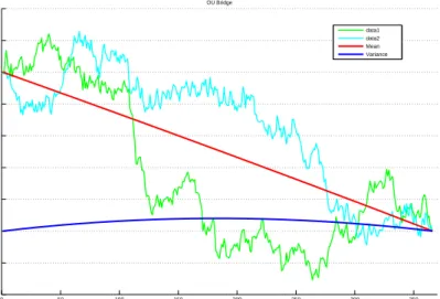
σ = 0, r = 0.05, T = 1. The number of steps is 365. This simulation shows the daily price movement for a year, when σ= 0. . . 40 2.3 Nine sets of ten sample paths of the commodity price process, with
vari-able parameters σ (rate at which information is revealed to market par-ticipants) ranging from 0.01 to 1 (value increases from top to bottom and left to right), and the following parameters: S0 = 75,S∞= 60, ψ= 0.3,
κ = 0.03,r = 0.05, T = 1. The number of steps is 365. This simulation shows the daily price movement for a year, for a range of values forσ. . . 40 2.4 Brent crude daily spot price from 4 November 2008 to 20 April 2010
(black path) plotted against five simulated paths from the model, with the following parameters: S0 = 62.78, S∞ = 60, ψ = 0.4, κ = 0.05,
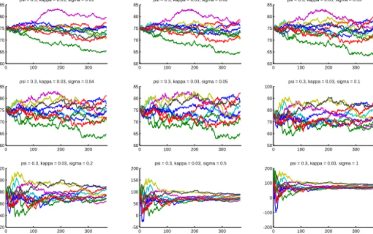
r = 0.025,T = 1. The number of steps is 365. . . 41 3.1 Commodity call option price surface as a function of the initial asset price
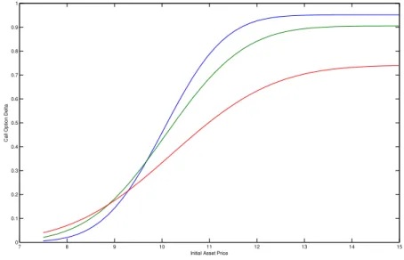
in the OU model and the time to maturity of the option. The parameters are set as follows: κ = 0.15, θ ranges from 0.3 to 0.8 with increments of 0.01, σ = 0.25, X0 = 0.6,ψ= 0.15, r= 0.05, and K = 10. The range of the maturities is from T = 0 to T = 3.0. . . 47 3.2 The commodity call option delta as a function of the initial asset price in
the OU model. The parameters are set as follows: κ= 0.15,θranges from 0.3 to 0.8 with increments of 0.01,σ = 0.25,X0= 0.6,ψ= 0.15,r= 0.05, and K = 10. The three maturities are T = 0.5 (blue), T = 1.0 (green), and T = 3.0 (red). . . 48
6.1 Mutual information in the case of Brownian noise. The mutual informa-tion I measures the amount of information contained in the observation about the value of the unknown signal X. At time zero, no data is avail-able so that the accumulated information content is zero. However, as time progresses, data is forthcoming that enhances the knowledge of the observer. Eventually, sufficient information, equivalent to the amount of the initial uncertainty−P
ipilnpi, is gathered, at which point the value
ofXis revealed. Strictly speaking this happens asymptotically ast→ ∞, although for all practical purposes the value of X will be revealed with high confidence level after a passage of finite amount of time. In this ex-ample, the parameters are chosen to bex1= 1,x2 = 2,p1= 0.4,p2= 0.6, and T = 50. The initial entropy (asymptotic value ofI) in this example is approximately 0.67. . . 103 6.2 Mutual information in the case of Poisson noise. The mutual information
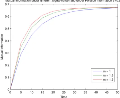
I measures the amount of information contained in the observation about the value of the unknown signal X. At time zero, no data is available so that the accumulated information content is zero. As time progresses, data is forthcoming that enhances the knowledge of the observer. Even-tually, a sufficient amount of information, equivalent to the amount of the initial uncertainty −P
ipilnpi, is gathered, at which point the value of
X is revealed. Strictly speaking this happens asymptotically as t→ ∞, although for all practical purposes the value of X will be revealed with high confidence level after a passage of finite amount of time. In this example, the parameters are chosen to be x1 = 1, x2 = 2, p1 = 0.4,
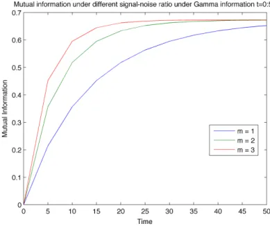
p2 = 0.6, and T = 50. The three plots corresponds to m = 1, m = 1.3 and m= 1.5. The initial entropy (asymptotic value ofI) in this example is approximately 0.67. . . 107 6.3 Mutual information in the case of the gamma noise. The mutual
informa-tion I measures the amount of information contained in the observation about the value of the unknown signal X. At time zero, no data is avail-able so that the accumulated information content is zero. However, as time progresses, data is forthcoming that enhances the knowledge of the observer. Eventually, a sufficient amount of information, equivalent to the amount of the initial uncertainty−P
ipilnpi, is gathered, at which point
the value ofX is revealed. Strictly speaking this happens asymptotically as t→ ∞, although for all practical purposes the value of X will be re-vealed with high confidence level after a passage of finite amount of time. In this example, the parameters are chosen to bex1= 1,x2 = 2,p1= 0.4,
p2 = 0.6, andT = 50. The three plots corresponds to m= 1, m= 2 and
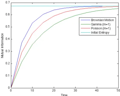
m = 3. The initial entropy (asymptotic value of I) in this example is approximately 0.67. . . 113 6.4 Mutual information comparison. The time dependence of the mutual
in-formationI is compared for three types of information processes: Brow-nian, Poisson, and gamma. The common parameters are chosen to be
x1 = 1, x2 = 2, p1 = 0.4, p2 = 0.6, and T = 50. Since other pa-rameters embody different meanings, a direct comparison as shown here need not reveal quantitative information. Nevertheless, the intuition one gains from the figure is that the revelation of the modulation signal in the Poisson information is somewhat slower than that in the drift for the Brownian information and the scale for the gamma information. . . 114
Theory of Information-Based
Commodity Pricing
Introduction
1.1
Models for commodity pricing
The starting point of most derivative pricing models—including those for commodity derivatives—is the specification of the price process of the underlying asset—for example, a geometric Brownian motion. More generally, the outcome of chance in the economy is often modelled by a probability space equipped with the filtration generated by a multi-dimensional Brownian motion, and it is assumed that asset prices are Ito processes that are adapted to this filtration. This particular example is, of course, the “standard” model within which a great deal of modern financial engineering has been carried out. A basic methodological problem with the standard model (and the same applies to various generalisations thereof involving jump processes) is that the market filtration is fixed once and for all. In other words, the filtration, which represents the unfolding of information available to market participants, is modelled first, in an essentially ad hoc
manner, and then it is assumed that the various asset price processes are adapted to it. But no indication is given about the nature of the “information” implicit in this setup, and it is not obvious at the beginning why Brownian motion, for example, should be regarded as providing information, rather than mere noise, in models constructed in this way.
In the real world—and this is certainly true in the world of commodity trading—the information available to market participants concerning the likely future cash flows as-sociated with an asset is essential to market participants when they make their decisions to buy or sell that asset. A change in such information or the arrival of such information will typically have an effect on the price at which market participants are willing to buy, or to sell, even if the agent’s preferences remain fundamentally unchanged.
Suppose, for example, that a trader working for a firm that holds crude oil in its inventory is thinking of selling a quantity of it at a price that seems attractive. Then along comes a news article drawing attention to the possibility of a shortage of crude oil three months hence. After some reflection, the trader decides it is no longer attractive to sell at that price; the alternative of holding on to the inventory for another three months, even taking into account the cost of carrying the inventory forward, is better. As a result, the trader declines the transaction. This trader is not alone in reaching such a decision, and the price for immediate delivery will increase whereas the price for delivery in three months will drop since the shortages have been eased as a consequence of stock piling. We take the view that the movement of the price of an asset should, therefore, be regarded as anemergent phenomenon, stimulated by information flows. That is, the price process of an asset should be viewed as the output of the various decisions made relating to possible transactions in the asset: these decisions in turn should be understood as being induced primarily by the flow of information to market participants.
1.2
Information-based approach
There is an extensive literature concerned with the modelling of commodity prices and commodity derivatives, approaching the problem from various different perspectives, backed up by a variety of empirical considerations. We mention, for example, the work of Working (1949), Brennan (1958), Brennan & Schwartz (1985), Brennan (1986), Wright & Williams (1989), Gibson & Schwartz (1990), Deaton & Laroque (1992), Pindyck (1993), Bessembinder et al. (1995), Schwartz (1997), Hilliard & Reis (1998, 1999), Miltersen & Schwartz (1998), Fackler & Tian (1999), Schwartz & Smith (2000), Bj¨ork & Land´en (2000), Yan (2002), Koekebakker & Lien (2004), Miltersen (2003), Cherian, Jacquier & Jarrow (2004), Nielsen & Schwartz (2004), Casassus & Collin-Dufresne (2005), Mellios (2006), and Jarrow (2010), and the general overviews provided by Duffie (1989) and Geman (2005).
In the theory of commodity pricing presented in Part I of the thesis, which is based on the approach set out in Brody, Hughston & Yang (2013b), we use the concept of market information about future supply and demand as a valuation basis for commodities and commodity derivatives. We shall be concerned here primarily with those commodities that can be physically stored, so we can assume the existence of the so-called convenience yield. Brennan (1991) defines the net convenience yield as “the flows of services accruing to the holder of the physical commodity, but not to the owner of a futures contract”. Indeed, physical inventory provides certain basic elements of service such as offering the owner the possibility (a) to avoid shortage of the spot commodity and thus to maintain
any production dependent upon it, or (b) to benefit from an anticipated future price increase. Generally speaking, the convenience yield represents, in percentage terms, the residual “benefit” conferred upon or derived by the owner of the commodity by virtue of its possession, after storage costs (explicit or implicit), insurance, and the like, have been duly taken into account.
The notion of a convenience yield, treated as a net “dividend” yield paid in effect to the owner of the physical commodity, drives the relation between the spot prices and the futures prices for many commodities (Brennan 1986, Fama & French 1987, 1988). It is reasonable to assume that an inverse relation holds between the overall inventory levels of a commodity and the associated convenience yield. Given the fact that inventories fluctuate, this indicates that the assumption of a constant convenience is in general likely to be an invalid one, and hence that a stochastic approach to convenience yield is needed in the modelling of oil prices (Brennan 1986, Gibson & Schwartz 1990).
In our approach to commodity spot prices we shall assume that the possession of one unit of commodity provides a “convenience dividend” equivalent to a continuous cash flow given by a random process{Xt}t≥0. Note that we are starting from the spot price
because physical ownership of the commodity is required in order to accumulate the “convenience dividend”. Note also that we shall be working directly with the actual flow of convenience from the storage or “possession” of the commodity, rather than the convenience yield. The point is that the convenience yield is in some respects a secondary notion since it depends on the price, which is what we are trying to determine. This is why we refer to{Xt}as a convenience dividend. Generally speaking, we take the view that in some ways it is more natural and more fundamental to model the convenience dividend than the convenience yield.
When a storable commodity is consumed, one can think of it as being exchanged for a consumption good of identical value—think of the difference between a bottle of wine (of known type and quality) which has not yet been opened, and an opened bottle of the same wine—the former is a storable good and the latter, once opened, becomes a “consumption” good. Following this line of argument, Jarrow (2010) takes the view that the value of a commodity derives in part from the element of optionality implicit in the timing of the conversion of the commodity from (in our language) a storable good to a consumption good. From this point of view, one can argue that the convenience yield in effect monetizes the value of the “option to consume’ in the form of a cash-flow stream, in some respects similar to the way that in credit theory a randomly timed credit event (the option of the bond issuer to default) is effectively monetized in the form of a (negative) continuous cash flow over the life of the credit risky product—thus leading to valuation formulae where the discounting is carried out not with respect to
the short rate, but rather with respect to the short rate augmented by the hazard rate for the credit event. In the case of commodities, the “consumption” event is a “good” outcome rather than a “bad” one, so when it is monetized over the life of the storable commodity the effect is to diminish the effective short rate used for discounting, rather than to enhance it, and that can be understood as the origin of the so-called convenience yield as a tool for modelling the dynamics of commodities.
In what follows, the convenience dividend (the existence of which we assume) will be modelled explicitly as a stochastic process, as we have indicated. In addition, to address the importance of forward looking information, we introduce a so-called market infor-mation process concerning future supply and demand, inventory, and overall market sentiment. The market filtration is assumed to be generated jointly by the convenience dividend process and the market information process. One can interpret the knowledge of the convenience dividend as providing information about current and past dividend levels, whereas the information process gives partial or speculative information about the future dividend flow.
The spot price of the commodity is given in the information-based approach by the discounted expected value of the cumulative future convenience dividends, conditional on the information provided by the market filtration. In the information-based framework, the filtration is modelled in a non-trivial way, so as a consequence the resulting dynamics for the prices is of a novel character. Nevertheless, the resulting scheme has a good deal of tractability, and in the case where convenience dividend is modelled by an Ornstein-Uhlenbeck process, we are able to derive closed-form expressions both for the underlying spot price and for the associated European option pricing formula.
1.3
Review of information-based asset pricing framework
1.3.1 OverviewCertain aspects of the BHM framework were originally developed a number of years ago as part of an attempt to gain a better understanding of the evolution and dynamics of quantum states in the presence of quantum noise (Brody & Hughston 2002; see also Adler, Brody, Hughston & Brun 2001, Brody & Hughston 2005, 2006). The ideas arising in these early investigations were redeveloped and extended by use of a novel Brownian-bridge technique in such a way as to provide a new approach to asset pricing. The first applications of the new approach were to the pricing and hedging of credit risky assets (Macrina 2006, Brody, Hughston & Macrina 2007). Since then the framework has evolved much further, and has found applications to equity pricing and stochastic
volatility (Brody, Hughston & Macrina 2008a, Filipovic, Hughston & Macrina 2012), reinsurance contracts (Brody, Hughston & Macrina 2008b, Hoyle 2010, Hoyle, Hughston & Macrina 2011), interest rates and inflation (Hughston & Macrina 2008, 2012, Macrina & Parbhoo 2011), statistical arbitrage trading (Brody, Davis, Hughston & Friedman 2009), signal processing (Brody, Hughston & Yang 2013a), and heterogeneous markets (Brody & Hughston 2013), as well as further applications to credit (Rutkowski & Yu 2007, Brody, Hughston & Macrina 2010).
The BHM framework can in some respects be seen as part of a larger program with an extensive literature being pursued by a number of authors exploring the role of incomplete information in finance, and attempting under various assumptions to model how prices are determined in such a setting, and how investment strategies should be best formulated. We mention, for example, the work of Gennotte (1986), Detemple (1986, 1991), Veronese (2000), Duffie & Lando (2001), Giesecke & Goldberg (2004), Jarrow & Protter (2004), Gombani, Jaschke & Runggaldier (2005), Coculescu, Geman & Jeanblanc (2008), Frey & Schmidt (2009), Bj¨ork, Davis & Land´en (2010), and Duffie (2012).
As we have remarked, the BHM framework regards the movements of the price of an asset as an emergent phenomenon. The price process of an asset is to be thought of as the output of the decisions made relating to possible transactions in the asset, and these decisions in turn is understood as being induced primarily by the flow of information to market participants. In other words, the BHM framework for asset pricing is based on modelling of the flow of market information. The information is that concerning the values of the future cash flows associated with the given assets, based upon which market participants determine estimates for the value of the right to the impending cash flows. These estimates in turn lead to the decisions concerning transactions that eventually trigger movements in the market quoted price.
Perhaps the most important difference between general pricing methods and the BHM framework is the following: in the BHM framework the stochastic process that governs the dynamics of an asset is deduced rather than imposed. In particular, rather than being imposed at the beginning of the modelling process in an arbitrary way, the dynamics of the asset are deduced as a consequence of the modelling of (a) the actual cash flows delivered by the asset, and (b) the associated flows of information relating to these random payments. The BHM framework is fully consistent with the general principles of arbitrage-free pricing theory. We present a brief synopsis of the BHM framework below, following the treatment of Brody, Hughston & Macrina (2007, 2008a).
1.3.2 Modelling framework
The BHM asset pricing framework requires three ingredients: (i) the cash flows; (ii) the investor risk preferences; and (iii) the flow of information available to market partici-pants. To incorporate these ingredients into the modelling process, one needs to translate them into mathematical terms, namely: (a) cash flows are modelled as random variables; (b) investors risk preference are modelled with the determination of a pricing kernel; and (c) the market information flow is modelled with the specification of a market filtration. The modelling process proceeds by the specification of a probability space (Ω,F,Q), on which a filtration {Ft}0≤t<∞ is constructed such that {Ft} can be identified as the market filtration. All asset price processes and other information-providing processes accessible to market participants will be adapted to {Ft}. The probability measure Q denotes the risk-neutral measure. The framework assumes the absence of arbitrage and the existence of a pricing kernel. With these conditions the existence of a unique preferred risk-neutral measure is ensured.
For simplicity, it is assumed that the default-free system of interest rates is deterministic (this condition is relaxed in Rutkowski & Yu 2007). The absence of arbitrage then implies that the default free discount bond system, denoted by {PtT}0≤t≤T <∞, can be written in the formPtT =P0T/P0t. The discount function {P0t}0≤t<∞is assumed to be differentiable and strictly decreasing, and to satisfy 0< P0t<1 and limt→∞P0t= 0.
1.3.3 Modelling the cash flows and the market information
We consider a single isolated cash flow occurring at time T, represented by a random variableXT. The valueStof the cash flow at any earlier timetin the interval 0≤t≤T is given by the discounted conditional expectation of XT:
St=PtTEQ[XT| Ft]. (1.1)
The value of the cash flow will be revealed at time T. It is reasonable to assume that some partial information regarding the value of the cash flow XT is available at earlier time, and this information will in general be imperfect. We therefore wish the market filtration to fulfil the properties that Ft fort < T embodies partial information concerning the valueXT of the impending cash flow, and that XT isFT-measurable. With these objective in mind, we proceed as follows. The flow of information available to market participants about the cash flow is assumed to be contained in a process
{ξt}0≤t≤T defined by
ξt=σtXT +βtT. (1.2)
The process{ξt}is referred to as themarket information process, or simply the informa-tion process. Observe that information process is constructed by two components. The first term σtXT contains the “true information” about the value of the cash flow XT, and is assumed here for simplicity to grow linearly in time at a rate σ. The parameter
σ can therefore be thought of as representing the signal-to-noise ratio; that is, the rate at which information about the true value ofXT is revealed as time passes. If σ is low, then the value of XT is effectively hidden until very near the time T of the occurrence of the cash flow. Ifσ is high, then the value of the cash flow is for all practical purposes revealed before T. The second term is given by the process {βtT}0≤t≤T, which is as-sumed to be a standard Brownian bridge over the time interval [0, T]. It is well-known that Brownian bridge process is a Gaussian process with mean zero, and the covariance of βsT and βtT is given by s(T −t)/T fors≤t. Also we have β0T = 0 andβT T = 0. In the information-based framework it is assumed that the cash flowXT and the process
{βtT} are independent. Therefore, the information contained in the bridge process represents “pure noise”. The market filtration{Ft}is thus assumed to be generated by the market information process:
Ft=σ({ξs}0≤s≤t). (1.3)
An immediate consequence of this setup is thatXT is FT measurable, but notFt mea-surable for t < T. Thus, as required, the value of XT becomes “know” at time T, but not earlier. The bridge process cannot be accessed directly by the market participants because it is not Ft-measurable for t < T. This is consistent with the fact that un-til the cash is paid at time T, the market participants cannot fully extract the “true information” about XT from the noisy information in the market.
1.3.4 Asset price processes
Having constructed the market information structure in the case of a single cash flow, we proceed, following BHM, to calculate the associated price process introduced in (1.1). It will be assumed that thea priori probability distribution of the cash flow XT is known. Let us further assume that XT has a density function p(x). Note, for convenience of demonstration and continuity with the materials to come later in this thesis, that
although we consider here the example of a continuous random variable XT, the result are equally applicable to random variables with more general distributions.
The determination of the asset price simplifies if we make note of the fact that the information process {ξt} is Markov. This can be seen by noting that
Q(ξt≤x|ξs, ξs1, ξs2, ..., ξsk) =Q ξt≤x|ξs, ξs s − ξs1 s1 ,ξs1 s1 −ξs2 s2 , ...,ξsk−1 sk−1 −ξsk sk =Q ξt≤x|ξs, βsT s − βs1T s1 ,βs1T s1 −βs2T s2 , ...,βsk−1T sk−1 −βskT sk
for s1 ≤ s2 ≤ · · · ≤ sk ≤ s ≤ t. Now it is a property of a Brownian bridge that the random variables βtT and βsT/s−βs1T/s1 are independent, and more generally that
βsT/s−βs1T/s1 andβs1T/s1−βs2T/s2 are independent. It follows that
Q(ξt≤x|ξs, ξs1, ξs2, ..., ξsk) =Q(ξt≤x|ξs) (1.4)
for arbitrary s1 ≤ s2 ≤ · · · ≤ sk ≤ s ≤ t. In addtion, from the fact that XT is FT measurable, we deduce that fort≤T, we have
St=PtTEQ[XT|ξt] =PtT
Z ∞
0
xπt(x)dx, (1.5)
whereπt(x) is the conditional probability density function for the random variableXT:
πt(x) = d
dxQ(XT ≤x|ξt). (1.6)
Note that by using a form of the Bayes formula, we can work out the conditional prob-ability density process for the cash flow:
πt(x) = R∞p(x)ρ(ξt|XT =x)
0 p(x)ρ(ξt|XT =x) dx
. (1.7)
Since βtT is a Gaussian random variable with mean zero and variance t(T −t)/T, and since that conditional on XT =x we have
ρ(ξt|XT =x) =Q(βtT < ξt−σXTt|XT =x), (1.8) we deduce that the conditional probability density forξt is:
ρ(ξt|XT =x) = s T 2πt(T−t) exp − (ξt−σtx)2T 2t(T−t) ! . (1.9)
It follows by inserting this into the Bayes formula (1.7) that πt(x) = p(x)exp h T T−t σxξt− 1 2σ2x2t i R∞ 0 p(x)exp h T T−t σxξt− 1 2σ2x2t i dx . (1.10)
Hence, the price process{St}0≤t≤T can be expressed in the form:
St=PtT R∞ 0 xp(x)exp h T T−t σxξt− 1 2σ2x2t i dx R∞ 0 p(x)exp h T T−t σxξt− 1 2σ2x2t i dx . (1.11)
1.3.5 Asset price dynamics
In standard approaches to asset pricing, the starting point is the specification of the price process in the form of a stochastic differential equation. In the BHM approach, the price process is directly deduced from the specification of the cash flow as well as the market filtration. Having obtained the price process (1.11), however, it will be of interest to identify to which stochastic differential equation (1.11) is the solution. To investigate this, let us define
XtT =EQ[XT|ξt]. (1.12)
From the foregoing calculation it should be evident that we can expressXtT in the form
XtT =X(ξt, t), where X(ξt, t) is defined by X(ξt, t) = R∞ 0 xp(x)exp h T T−t σxξ− 1 2σ 2x2ti dx R∞ 0 p(x)exp h T T−t σxξ− 1 2σ2x2t i dx . (1.13)
An application of Ito’s lemma shows that the dynamical equation for XtT is given by
dXtT = σT T −tVt 1 T−t(ξt−σT XtT) dt+ dξt . (1.14)
Here Vt is the conditional variance of the cash flow XT:
Vt=Et h (XT −Et[XT])2 i = Z ∞ 0 x2πt(x)dx− Z ∞ 0 xπt(x)dx 2 , (1.15)
whereEt[−] denotes the conditional expectationEQ[−|ξt]. We proceed further by defin-ing the new process{Wt}0≤t≤T according to
Wt=ξt−
Z t
0
1
and substitute this back into equation (1.14). Then we have dXtT =
σT
T−tVtdWt. (1.17)
It follows from the expression for the price process and the relation that
dPtT =rtPtTdt, (1.18)
wherertdenotes the short rate, the dynamics of the price process is
dSt=rtStdt+ ΣtTdWt, (1.19) where
ΣtT =PtT
σT
T −tVt (1.20)
is the absolute volatility process.
It is a straightforward exercise to check the process {Wt} defined in equation (1.16) is a (Q,Ft)-Brownian motion. One can check this by use of the L´evy characterisation of the Brownian motion, that is, to check that {Wt} is a (Q,Ft)-martingale and that the quadratic variation of {Wt}is t.
It is interesting to observe that in the BHM framework we have been able to derive the Brownian motion that drives the price process. In particular, it is a nonlinear functional of the history of the information process, which in turn depends on the future cash flow of the asset, as well as on ambient noise. This observation shows that the “standard” interpretation, that random movements of prices are generated by noise, is perhaps not satisfactory. Indeed, in Macrina (2006) and Brody et al. (2008a) it is shown that the geometric Brownian motion model used in the Black-Scholes theory can be derived from a market information process consisting of a normal random variable for the log-return of the asset determining the “signal” component, and an independent Brownian bridge for market noise.
1.3.6 European call option pricing formula
The information-based framework can be used to price various financial derivatives, in spite of the apparent sophisticated form (1.11) of the price process. For the purpose of illustration, we consider the valuation of a European call option written on a asset for which the dynamics of the price process is given by equation (1.19). The option has strike price K and matures at time t; the underlying asset pays a single cash flow at
timeT > t. Given this setup, we can write down the initial value of this option as
C0 =P0tEQ(St−K)+
. (1.21)
Substitute the expression forSt into the above formula we obtain
C0 =P0tEQ " PtT Z ∞ 0 xπt(x)dx−K +# . (1.22)
For simplicity, let us denote the conditional probabilityπt(x) of (1.10) in the form
πt(x) = R∞pt(x)
0 pt(x)dx
, (1.23)
where the unnormalised density processpt(x) is defined by
pt(x) =p(x)exp T T −t σxξt− 1 2σ 2x2t . (1.24)
Given these ingredient, we can rewrite the expression forC0 as
C0=P0tEQ " 1 Ψt Z ∞ 0 pt(x) (xPtT −K) dx +# , (1.25) where Ψt= Z ∞ 0 pt(x)dx. (1.26)
It can be shown that the factor 1/Ψt appearing in (1.25) is a (Q,Ft)-martingale, and can be used as a change of measure density martingale. This can be seen as follows. First, from (1.24) we have
dpt(x) = σT T−txpt(x) dξt+ 1 T−tdt , (1.27) and hence dΨt Ψt = σT T −tXtT dξt+ 1 T −tdt . (1.28)
It follows, on account of the Ito lemma, that dΨ−t1
Ψ−t1 =−
σT
T −tXtTdWt, (1.29)
where we have substituted (1.16). Since {Wt} is a Q-Brownian motion, the desired conclusion follows.
By using {Ψ−t1} a new measure B on (Ω,Ft), which will be called a “bridge measure”. The option price can then by written in the new measure as
C0 =P0tEB " Z ∞ 0 pt(x) (xPtT −K) dx +# . (1.30)
What is special about the bridge measure B is that under this measure, the process
{ξt} is Gaussian with mean zero and variancet(T−t)/T. That is to say, under B, the information process{ξt}is a standard Brownian bridge. Furthermore, sincept(x) can be written as a function ofξt, which isB-Gaussian, we are able to carry out the expectation and obtain a tractable formula for value of the option. In order to determine the option price, define for each t, T, and K a constant ξ∗, which is a unique critical value of ξt such thatSt=K when ξt=ξ∗. This implies the following condition:
Z ∞ 0 p(x)exp T T −t σxξ∗−1 2σ 2x2t (xPtT −K) dx= 0. (1.31)
Together with the fact thatξt isB-Gaussian, we can perform the Gaussian integration explicitly and find the option price:
C0 =P0t Z ∞ 0 xp(x)N −z∗+σx√τdx−P0tK Z ∞ 0 p(x)N −z∗+σx√τdx. (1.32) Here N(z) denotes the cumulative distribution function of a standard normal random variable, and τ = tT T −t, z ∗=ξ∗ s T t(T−t). (1.33)
We see, therefore, that in spite of the elaborate model (1.11) for the price process, the option pricing formula reduced to something that is analogous to that of Black and Scholes, albeit requiring the relatively simple numerical determination of the solutionξ∗
of (1.31) and performing the integration (1.32).
1.3.7 Applications to commodity prices
In what follows, the goal is to apply the BHM method to commodities. Some rethink-ing of the BHM technique is required, since the convenience dividend of a commodity supplies, in effect, constitutes a continuous cash flow, as opposed to a single cash flow occurring at a prefixed future time in the example considered above. Nevertheless, under appropriate assumptions we are able to obtain exact solutions.
The structure of the remainder of the material in this part of the thesis is as follows. In section2.2-2.3we introduce the model for the convenience dividend and for the market filtration. Some useful facts about the mean-reverting Ornstein-Uhlenbeck (OU) process are recalled in section 2.4, in particular, various features of the OU bridge are outlined in section 2.4.2. These are used in the derivation of the commodity price process. In section2.8, we derive the stochastic differential equation satisfied by the price process. In doing so, we are able to obtain an innovations representation for the associated filtering problem in closed form. Simulation studies of the price process are presented for various values of the model parameters. We work out pricing formulae for call options on the underlying spot price in proposition3.1.1. In section3.3, the model is applied to obtain the corresponding price processes for futures contracts, which are useful since futures contracts are very commonly traded in commodity markets. The formulae developed thus far have made use of a simplifying assumption to the effect that the parameters of the model are constant in time. We know, however, from various other models for derivative pricing, that it can be highly advantageous to introduce “time dependent” parameters into the model, to open up the possibility of calibration of the model to various market instruments. Therefore, with this point of view in mind, in section 3.4 we proceed to extend the model to a time-inhomogeneous setup. The resulting formulae in the time-dependent situation are of course of rather greater complexity, but the overall modeling scheme remains analytically tractable, as will be demonstrated.
Commodity Prices
2.1
Chapter overview
In this chapter, an information-based continuous-time model for the prices of storable commodities is introduced. The model employs the concept of market information about future supply and demand as a basis for valuation. The physical ownership of commodi-ties is regarded as providing “convenience dividends” equivalent to cash flows. The market filtration is assumed to be that generated by the aggregate of (i) an information process concerning the future convenience dividend flow; and (ii) a convenience dividend process that provides information about current and past dividend levels. The price of a commodity is given by the risk-neutral expectation of the discounted cumulative future convenience dividends, conditional on the information provided by the market filtration.
2.2
Model setup
As indicated in the introduction, the starting point of the BHM framework is the specifi-cation of: (a) the random variables (called “market factors”) determining the cash flows associated with a given asset, and (b) the flow of information to market participants concerning these market factors. The models that have been considered so far under this framework have the property that the cash flows occur at pre-specified times. The specification of the market factors and the associated information processes for such dis-crete cash flows is useful for the modelling of many different types of financial contracts. The purpose of the present approach to storable commodity pricing is to introduce an extension of the framework to the situation where an asset pays a continuous dividend.
As an illustrative example we consider, in particular, the case for which the cash flow is an Ornstein-Uhlenbeck process {Xt}. As usual we begin with the probability space (Ω,F,P), wherePdenotes the market measure. We assume the absence of arbitrage, and that a pricing kernel{πt}has been established. These assumptions ensure the existence of a unique preferred pricing measure (the risk neutral measure), which will be denoted by Q.
Based on these assumptions, the value at timetof the storable commodity that generates a continuous stream of benefit equivalent to the cash flow {Xt} is given by the pricing formula St= 1 πtE P t Z ∞ t πuXudu . (2.1)
Equivalently, transforming to the risk-neutral measure, we can write
St= 1 PtE Q t Z ∞ t PuXudu , (2.2) where Pt= exp − Z t 0 rsds (2.3) is the discount factor, with the associated short rate {rt}. In what follows, we shall use EQ[−] or E[−] to represent the expectation under the risk-neutral measure Q. For simplicity of exposition, let us assume that the interest rate system is deterministic. Once we work things out for deterministic {rt} then we can consider the more general situation. From this assumption, we havePt=P0t, where {P0t}t≥0 are initial prices of
discount bonds. We shall further assume that the market filtration is generated jointly by the following processes:
(a) the convenience dividend process {Xt}t≥0; and (b) an “information process” {ξt}t≥0 of the form:
ξt=σt
Z ∞
t
PuXudu+Bt, (2.4)
whereQ-Brownian motion {Bt}is independent of {Xt}.
In other words, at timetthe market filtration Ft is generated by:
Ft=σ({Xs}0≤s≤t,{ξs}0≤s≤t). (2.5) We can interpret the choice of market filtration as arising from the following two com-ponents:
• The knowledge of the convenience dividend{Xt}, providing information about the
current andpast dividend levels.
• The information process {ξt}, providing partial information about the future
dividend flow.
2.3
Modelling the convenience dividend
Motivated in part by the pioneering work of Gibson & Schwartz (1990, 1991), in which the convenience yield is assumed to follow a mean-reverting process, we shall introduce a simple model for the commodity convenience dividend. Specifically, we consider the case for which {Xt}is an Ornstein-Uhlenbeck (OU) process.
We shall begin by considering the constant parameter case so that we have the following mean-reverting dynamics for the convenience dividend in the risk neutral measure:
dXt=κ(θ−Xt)dt+ψdβt, (2.6) with initial condition X0. Here {βt} is a Q-Brownian motion that is independent of
{Bt},θ is the mean reversion level, κ is the mean reversion rate, andψ is the dividend volatility. We shall look at the constant parameter (time homogeneous) case first, and then extend the results into time-dependent (time inhomogeneous) situation. The linear stochastic equation (2.6) can easily be solved to yield the solution
Xt= e−κtX0+θ(1−e−κt) +ψe−κt
Z t
0
eκsdβs. (2.7)
An elementary way of establishing this is to apply Ito’s lemma onf(Xt, t) =Xteκt. The Gaussian process (2.7) is fully specified by its mean
E[Xt] = e−κtX0+θ(1−e−κt) (2.8)
and the covariance
Cov[Xt, XT] =
ψ2
2κe
−κT(eκt−e−κt). (2.9)
In particular, settingT =tin (2.9) we find that
Var[Xt] =
ψ2
2κ(1−e
2.4
Properties of the Ornstein-Uhlenbeck process
In what follows we present some elementary but perhaps not entirely obvious properties of the OU process, which will be required for the subsequent commodity pricing analysis. In particular, here we highlight two orthogonal decomposition properties of the OU process.
2.4.1 Reinitialization and orthogonal decomposition
We begin by noting that the OU process possesses the reinitialisation property in the sense that
XT = e−κ(T−t)Xt+θ(1−e−κ(T−t)) +ψe−κT
Z T
t
eκudβu. (2.11) This follows from a direct substitution of (2.7). Now since{Xt}is a Gaussian process, by use of the variance-covariance relations, one can easily verify that the random variables
Xt and XT −e−κ(T−t)Xt are independent. This property implies that an OU process admits anorthogonal decomposition of the form
XT = (XT −e−κ(T−t)Xt) + e−κ(T−t)Xt, (2.12) forT > t. Note that when the mean reversion rateκ is set to zero this relation reduces to the usual independent increments decomposition for Brownian motion.
2.4.2 The Ornstein-Uhlenbeck bridge
Interestingly, there is another, perhaps somewhat less appreciated, orthogonal decom-position, associated with the OU process. This decomposition takes the form
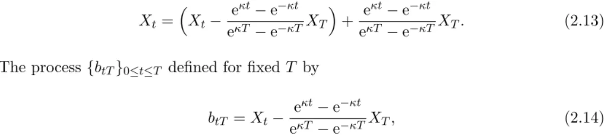
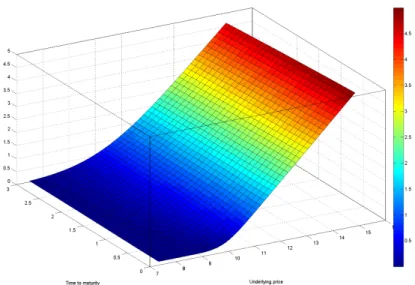
Xt= Xt− eκt−e−κt eκT−e−κTXT + e κt−e−κt eκT −e−κTXT. (2.13) The process {btT}0≤t≤T defined for fixed T by
btT =Xt−
eκt−e−κt
eκT −e−κTXT, (2.14)
appearing in the decomposition (2.13) is theOrnstein-Uhlenbeck bridge (OU bridge). Figure 2.1 shows sample paths of the OU bridge process, as well as its mean and vari-ance. With the help of the hyperbolic functions, we can expressing the OU bridge in the form
btT =Xt−
sinh(κt)
0 50 100 150 200 250 300 350 -0.2 -0.1 0 0.1 0.2 0.3 0.4 0.5 0.6 0.7 Time OU Bridge data1 data2 Mean Variance
Figure 2.1: Two sample paths of OU Bridge with the following parameters: X0= 0.5,
θ = 1.2, ψ = 0.4, κ= 0.2,T = 1. The number of steps is 365. The mean (red) and variance (blue) of the OU bridge are also plotted.
Clearly, we have that
b0T =X0 and bT T = 0. (2.16)
By use of the covariance relations, one can check thatbtT andXT are independent. Note that the OU bridge is a Gaussian process with mean
E[btT] = sinh(κ(T−t)) sinh(κT) X0+ 1−sinh(κt) + sinh(κ(T −t)) sinh(κT) θ, (2.17) and variance Var[btT] = ψ2 2κ cosh(κT)−cosh(κ(T −2t)) sinh(κT) . (2.18)
The main observation one can make about the OU bridge is the independence of btT and XT, which will become very useful in what follows when we prove the Markovian property of the generating processes of the joint filtration.
2.5
Commodity pricing formula
Putting together all the properties we have derived from the last few sections, we are now ready to calculate the price of the commodity. To achieve this, we need to focus on the expectation below:
St= 1 PtEt Z ∞ t PuXudu . (2.19)
Note that the conditioning here is with respect to the joint filtration (2.5). In general, performing such a conditional expectation is difficult. However, we have the following result that simplifies the computation considerably.
Proposition 2.5.1. The information process{ξt} and the convenience dividend process
{Xt} are jointly Markovian, implying that, the following relation holds:
E Z ∞ t PuXudu {ξs}0≤s≤t,{Xs}0≤s≤t =E Z ∞ t PuXudu ξt, Xt . (2.20)
The details of the proof of this proposition can be found in the AppendixA. From the orthogonal decomposition (2.12), we can isolate the dependence of the commodity price on the current level of the convenience dividend Xt and, remarkably, this turns out to be linear in our model.
In particular, we have the following decomposition of the discounted cumulative future dividend flow into orthogonal components:
Z ∞ t PuXudu= Z ∞ t Pu Xu−e−κ(u−t)Xt du+ Z ∞ t Pue−κ(u−t)du Xt. (2.21)
Note that the independence of the two terms on the right side of (2.21) can easily be checked by considering their covariance, since both terms are Gaussian. It follows from (2.2) and the orthogonal decomposition property that the commodity price can be expressed in the form:
StPt = E Z ∞ t Pu Xu−e−κ(u−t)Xt du ξt, Xt +E Z ∞ t Pue−κ(u−t)du Xt ξt, Xt . (2.22)
We now observe that, since the term Xu−e−κ(u−t)Xt
is independent ofXt, the con-ditioning with respect toXtin the first expectation in the right side of (2.22) drops out, and we obtain StPt=E[At|σtAt+Bt] + Z ∞ t Pue−κ(u−t)du Xt, (2.23) where At= Z ∞ t Pu Xu−e−κ(u−t)Xt du, (2.24)
and Bt is the value of the Brownian motion at time t. Note that σtAt+Bt = ξt. Now we are working with the expectation of the formE[A|A+B], whereA and B are independent Gaussian random variables, each with a known mean and variance. More
specifically, we have: A= Z ∞ t Pu Xu−e−κ(u−t)Xt du, (2.25) and B = Bt σt. (2.26)
In order to compute the expectation in (2.23), the following lemma will become useful.
Lemma 2.5.1. LetA,B be a pair of independent Gaussian random variables, and write
A=z(A+B) + (1−z)A−zB. (2.27)
Then A+B and (1−z)A−zB are orthogonal, and hence independent, if we set
z= Var [A]
Var [A] + Var [B]. (2.28)
Proof. SinceA+B and (1−z)A−zBare Gaussian random variables, it suffices to check that
Cov [(A+B),(1−z)A−zB] = 0. (2.29) After a straightforward calculation, we deduced that the necessary condition for (2.29) to hold is for z to be equal to (2.28).
It follows from the above lemma that isA and B are independent and Gaussian, and if
z is given by (2.28), then we have
E[A|A+B] =z(A+B) + (1−z)E[A]−zE[B]. (2.30)
To compute the conditional expectationE[A|A+B], we are thus required to work out the means and the variances of the random variablesAandB. To begin, let us consider
E[A] =E Z ∞ t Pu Xu−e−κ(u−t)Xt du . (2.31)
If we recall the reinitialisation property of the OU process
Xu = e−κ(u−t)Xt+θ(1−e−κ(u−t)) +ψe−κu
Z u
t
and substitute this in (2.31), then we find E[A] = E θ Z ∞ t Pu 1−e−κ(u−t)du+ψ Z ∞ t e−κuPu Z u t eκsdβsdu = θE Z ∞ t Pudu −θE Z ∞ t Pue−κ(u−t)du +ψE Z ∞ t e−κuPu Z u t eκsdβsdu . (2.33)
For the last term of (2.33), interchange order of integration. We have
ψE Z ∞ u=t e−κuPu Z u s=t eκsdβsdu = ψE Z ∞ s=t eκs Z ∞ u=s Pue−κudu dβs = 0. (2.34)
Therefore, we are left with the expression
E[A] = θE Z ∞ t Pudu −θE Z ∞ t Pue−κ(u−t)du = θ Z ∞ t Pudu−θ Z ∞ t Pue−κ(u−t)du. (2.35) Note also that
E[B] =E Bt σt = 0, (2.36)
whereBt is a standard Brownian motion. On the other hand, we have
A+B = Z ∞ t Pu Xu−e−κ(u−t)Xt du+Bt σt = Z ∞ t PuXudu− Z ∞ t PuXte−κ(u−t)du+ Bt σt = 1 σtξt−Xt Z ∞ t Pue−κ(u−t)du. (2.37) In order to simplify the calculation, let us introducept and qt according to
pt= Z ∞ t Pudu and qt= Z ∞ t Pue−κ(u−t)du. (2.38) We then have: PtSt= (1−zt) [θpt+qt(Xt−θ)] +zt ξt σt. (2.39)
Now from A−E[A] = ψ Z ∞ t eκs Z ∞ s Pue−κudu dβs = ψ Z ∞ t Z ∞ s Pue−κ(u−s)dudβs = ψ Z ∞ t qsdβs, (2.40)
we find that the variance ofA is
Var [A] = E h (A−E[A])2 i = ψ2E Z ∞ t qsdβs 2 = ψ2 Z ∞ t q2sds, (2.41)
on account of the Wiener-Ito isometry. The variance ofB is
Var [B] = Var Bt σ2t2 = 1 σ2t. (2.42)
Putting these together, we obtain the following explicit formula for the commodity price:
St= (1−zt)Pt−1[θpt+qt(Xt−θ)] +ztPt−1 ξt σt, (2.43) where zt= σ2ψ2tRt∞qs2ds 1 +σ2ψ2tR∞ t qs2ds , (2.44)
withptand qt given in (2.38).
Remark 2.5.1. From the expression of the weighting factor zt in (2.44), we see that for largeψ and (or) largeσ, the value ofzttends to unity. On the other hand, for small
ψ and (or) small σ, the value of zt tends to zero. Hence, if the market information has a low noise content, i.e. high information flow rate σ, then the market information is what mainly determines the price of the commodity. On the other hand, if the volatility of the convenience dividend is high, then market participants also rely heavily on “the best information about the future” in their determination of prices, rather than simply assuming that the current value of the dividend is a good guide to the future.
The other term, that is, the term proportional to (1−zt) in the expression for St is essentially an annuities valuation of a constant dividend rate set at the mean reversion level, together with a correction term to adjust for the present level of the dividend rate.
This term dominates in situations when the market information is of low quality. It also dominates in situations when the dividend volatility is low. In other words, in the absence of significant information concerning potential future return, our judgements are formed on the basis of a kind of average of the status quo and the market consensus regarding long term average. But we also rely on the status quo in situations where there is little uncertainty, i.e. when the dividend volatility is very low.
2.6
Special case of constant interest rates
Under the assumption of a constant interest rate, we can make further simplifications on the commodity valuation formulae (2.43) and (2.44). Whether this is a valid approx-imation or not depends on the application one has in mind, but in any case one gains insights by considering the constant interest rate situation. The discount bond price in this case becomes
Pt= e−rt. (2.45) Therefore, we have pt= 1 re −rt and q t= 1 r+κe −rt. (2.46)
Substituting this in (2.43), we find, after a short calculation, the pricing formula under constant interest rate setup takes the form
St= (1−zt)
κθ+rXt
r(r+κ) +zte rtξt
σt, (2.47)
with the weighting factor
zt=
σ2ψ2t
2r(r+κ)2e2rt+σ2ψ2t. (2.48) Remark 2.6.1. The following observations can be made from a closer inspection of the expression (2.47) for the commodity price:
1. The first term is a kind of annuitised weighted average of the mean reversion level and the current level of the dividend, multiplied by the weighting factor (1−zt). 2. If we set σ= 0, then the first term alone determines the price of the commodity. 3. The second term then modifies the price by bringing in the market information
2.7
Alternative derivation of commodity price process
In this section, an alternative derivation of the price process is presented. The purpose of this is to derive a number of other relations that in turn will provide a way of identifying the innovations arising in connection with the associated filtering problem. For this purpose, let us consider the case when interest rate is constant. Therefore, we havePtSt = Et Z ∞ t PuXudu =Et Z ∞ t e−ruXudu = Et Z ∞ 0 e−ruXudu − Z t 0 e−ruXudu. (2.49)
From (2.7) the integral term in the expectation in (2.49) can be simplified according to
Z ∞ 0 e−ruXudu = Z ∞ 0 e−ru e−κuX0+θ 1−e−κu +ψe−κu Z u 0 eκsdβs du = X0 Z ∞ 0 e−(r+κ)udu+ Z ∞ 0 θ e−ru−e−(r+κ)u du +ψ Z ∞ 0 e−(r+κ)u Z u 0 eκs dβs du. (2.50) Solving the first two integrals and rearrange terms, we get
Z ∞ 0 e−ruXudu = X0 r+κ+θ 1 r − 1 r+κ +ψ Z ∞ 0 e−(r+κ)u Z u 0 eκs dβs du = rX0+κθ r(r+κ) +ψ Z ∞ 0 eκs Z ∞ s e−(r+κ)u dudβs. (2.51)
For the double integral, one can use a change of variables to interchange the order of integration to yield: Z ∞ 0 e−ruXudu = rX0+κθ r(r+κ) + ψ r+κ Z ∞ 0 eκse−(r+κ)s dβs = rX0+κθ r(r+κ) + ψ r+κ Z ∞ 0 e−rs dβs. (2.52)
Then, substituting (2.52) back into (2.49), we have
PtSt = Et rX0+κθ r(r+κ) + ψ r+κ Z ∞ 0 e−rs dβs − Z t 0 e−ruXudu = Et rX0+κθ r(r+κ) + ψ r+κ Z ∞ t e−rs dβs+ ψ r+κ Z t 0 e−rs dβs − Z t 0 e−ruXudu = rX0+κθ r(r+κ) + ψ r+κ Z t 0 e−rs dβs + ψ r+κEt Z ∞ t e−rs dβs − Z t 0 e−ruXudu. (2.53)
The problem is now reduced to the determination of the conditional expectation E Z ∞ t e−rs dβs {ξs}0≤s≤t,{Xs}0≤s≤t . (2.54)
Before we begin to solve the problem, the following observations can be made. Recall that the model filtration is generated jointly by{ξt}and {Xt}. Furthermore,ξt can be expressed in the form:
ξt = σt Z ∞ t e−ruXudu+Bt = σt Z ∞ 0 e−ruXudu− Z t 0 e−ruXudu +Bt = σt rX0+κθ r(r+κ) + ψ r+κ Z ∞ 0 e−ru dβu− Z t 0 e−ruXudu +Bt = ωt+σt rX0+κθ r(r+κ) + ψ r+κ Z t 0 e−ru dβu− Z t 0 e−ruXudu . (2.55)
Here we have defined
ωt= σψt r+κ Z ∞ t e−ru dβu+Bt:= σψt r+κYt+Bt, (2.56) where Yt= Z ∞ t e−ru dβu. (2.57)
Note that the integrand in Yt is a deterministic function of time. Therefore, for each
t ≥ 0, Yt is a normal random variable. It is easy to see that the filtration generated jointly by {ξt} and {Xt} is equivalent to the filtration generated jointly by {ωt} and
{Xt}. Therefore, the conditional expectation appearing in (2.53) can be expressed in the form E Z ∞ t e−rs dβs {ξs}0≤s≤t,{Xs}0≤s≤t = E Z ∞ t e−rs dβs ωt = Z ∞ −∞ yπt(y)dy. (2.58)
Here we have made use of the facts that Yt is independent of {Xs}0≤s≤t, and that
{ωt} is Markov. We write πt(y) for the conditional density of the random variable Yt. Specifically, we have:
πt(y) = d
Note that the conditional density function of Yt can be worked out by using a form of the Bayes formula:
πt(y) = R p(y)ρ(ωt|Y =y)
p(y)ρ(ωt|Y =y)dy
. (2.60)
Here p(y) denotes the a priori density for Yt, which we shall work out shortly, and
ρ(ωt|Y = y) denotes the conditional density for the random variable ωt given that
Y =y. The fact that Yt is a Gaussian random variable means we only need the mean and variance to find out the a priori density p(y). After a straightforward calculation, we find thatYt has mean zero and variance e−2rt/(2r). Therefore,
p(y) = r re2rt π exp −re 2rty2 . (2.61)
Also the fact that Bt is a Gaussian random variable with mean zero and variance t implies that conditional onY =y,ωtis Gaussian with meanσψty/(r+κ) and variance
t. We thus deduce that the conditional density forωt is
ρ(ωt|Y =y) = r 1 2πtexp − ωt−rσψt+κy 2 2t . (2.62)
Inserting this expression into the Bayes formula we get thea posteriori density function:
πt(y) = p(y) q 1 2πtexp −(ωt− σψt r+κy) 2 2t R p(y) q 1 2πtexp −(ωt− σψt r+κy) 2 2t dy = p(y)exp h σψωt r+κy− 1 2 σ2ψ2t (r+κ)2y2 i R p(y)exp h σψωt r+κy− 1 2 σ2ψ2t (r+κ)2y2 i dy . (2.63)
It follows that for the conditional expectation we can write
E Z ∞ t e−rs dβs ωt = Z yπt(y)dy = R yp(y)exp h σψωt r+κy− 1 2 σ2ψ2t (r+κ)2y2 i dy R p(y)exphσψωt r+κy− 1 2 σ2ψ2t (r+κ)2y2 i dy . (2.64)
Substituting the a priori density p(y) defined in equation (2.61) into equation (2.64), we have (2.64) = R y exp h σψωt r+κy− 1 2 σ2ψ2t (r+κ)2 + 2re2rt y2 i dy R exp h σψωt r+κy− 1 2 σ2ψ2t (r+κ)2 + 2re2rt y2idy = R y eay−by2dy R eay−by2 dy , (2.65) where a= σψωt r+κ and b= 1 2 σ2ψ2t (r+κ)2 + 2re 2rt . (2.66)
Performing the integration, we thus obtain
E Z ∞ t e−rs dβs ωt = a 2b. (2.67)
Substituting aand bof (2.66) in here, we find
E Z ∞ t e−rs dβs ωt = σψωt r+κ σ2ψ2t (r+κ)2 + 2re2rt = (r+κ)σψωt 2r(r+κ)2e2rt+σ2ψ2t = r+κ σψt ztωt, (2.68) where zt= σ2ψ2t 2r(r+κ)2e2rt+σ2ψ2t (2.69)
is the weighting factor obtained in the previous method for the calculation presented earlier. Substituting (2.68) into (2.53), together with the fact that expression for the new information process{ωt} in terms of the previous one{ξt} is given by
ωt=ξt−σt rX0+κθ r(r+κ) + ψ r+κ Z t 0 e−ru dβu− Z t 0 e−ruXudu , (2.70)
we find that the pricing formula (2.53) then becomes
PtSt = rX0+κθ r(r+κ) + ψ r+κ Z t 0 e−rs dβs + ψ r+κEt Z ∞ t e−rs dβs − Z t 0 e−ruXudu. (2.71)
By use of equation (2.68), we can replace the conditional expectation term above and obtain: PtSt = rX0+κθ r(r+κ) + ψ r+κ Z t 0 e−rs dβs+ ψ r+κ r+κ σψt ztωt− Z t 0 e−ruXudu = rX0+κθ r(r+κ) + ψ r+κ Z t 0 e−rs dβs+ zt σtωt− Z t 0 e−ruXudu. (2.72)
Recalling the expression forωt from equation (2.56) and rearranging terms, we obtain:
PtSt = rX0+κθ r(r+κ) + ψ r+κ Z t 0 e−rs dβs− Z t 0 e−ruXudu + zt σt ξt−σt rX0+κθ r(r+κ) + ψ r+κ Z t 0 e−ru dβu− Z t 0 e−ruXudu .(2.73)
The various terms in equation (2.73) then cancel out or group together to give
PtSt = (1−zt) rX0+κθ r(r+κ) +zt ξt σt −(1−zt) Z t 0 e−ruXudu+ (1−zt) ψ r+κ Z t 0 e−ru dβu. (2.74)
Let us consider the expression Rt
0 e
−ruX
udu in equation (2.74). Since we know the expression for Xt, and the interest rate is constant, we can solve the integral:
Z t 0 e−ruXudu = X0−θ r+κ h 1−e−(r+κ)ti+ θ r 1−e −rt + ψ r+κ Z t 0 e−ru dβu− ψ r+κe −(r+κ)t Z t 0 eκudβu = rX0+κθ r(r+κ) + ψ r+κ Z t 0 e−ru dβu − e −rt r(r+κ) rX0e−κt+rθe−κt+rψe−κt Z t 0 eκudβu+κθ+rθ . (2.75)
After further cancellation and rearrangement of terms, we get
Z t 0 e−ruXudu = rX0+κθ r(r+κ) + ψ r+κ Z t 0 e−ru dβu− e−rt r(r+κ)(rXt−rθ+κθ+rθ) = rX0+κθ r(r+κ) + ψ r+κ Z t 0 e−ru dβu−e−rt κθ+rXt r(r+κ) . (2.76)
Inserting the above expression (2.76) in the pricing formula (2.74), we obtain PtSt = (1−zt) rX0+κθ r(r+κ) + (1−zt) ψ r+κ Z t 0 e−ru dβu +zt ξt σt−(1−zt) rX0+κθ r(r+κ) + ψ r+κ Z t 0 e−ru dβu−e−rt κθ+rXt r(r+κ) .
Finally, with further rearrangement of the various terms, we have
St= (1−zt)
κθ+rXt
r(r+κ) +zte rtξt
σt, (2.77)
which agrees with the result in equation (2.47) derived from the previous approach. In terms of the alternative information process{ωt}, the price process can be expressed in the form St = κθ+rXt r(r+κ) + e rtz t ωt σt, (2.78) where ωt = σψt r+κ Z ∞ t e−rudβu+Bt. (2.79) We see, therefore, that although this alternative derivation involves a somewhat more elaborate set of calculations, the end result is a relatively simple expression that is going to be very useful in the study below of the dynamics of the price process.
2.8
Price dynamics and innovation representation
In the previous sections, we have shown that the commodity price process can be ex-pressed in two different forms. In this section, we are going to use the simpler expression (2.78) to derive the price dynamics, and derive the innovations representation, which in turn provides the “observable” driving Brownian motion for the price.
Applying Ito’s lemma on the price process (2.78), we have
dSt = r r(r+κ)dXt+re rtz t ωt σtdt−e rtz t ωt σt2dt+ e rtωt σtdzt+ ertzt σt dωt. (2.80)
Recall that from equation (2.6), one gets
dSt = r r(r+κ)(κθdt−κXtdt+ψdβt) +r St− κθ+rXt r(r+κ) dt −ertzt ωt σt2dt+ e rtωt σtdzt+ ertzt σt dωt. (2.81)