A Fully Automated Method for Noisy cDNA Microarray Image
Quantification
Islam A. Fouad¹, Mai S. Mabrouk²*, Amr A. Sharawy³
1 College of Applied Medical Sciences, Salman Bin Abdul-Aziz University, Kharj, KSA.
Email:
[email protected]
2 Biomedical Engineering, Misr University for Science and Technology (MUST University), 6th of October,
Egypt.
Email:
[email protected]
3 Systems and Biomedical Engineering, Cairo University, Giza, Egypt.
Email:
[email protected]
ABSTRACT
DNA microarray is an innovative tool for gene studies in biomedical research, and its applications can vary from cancer diagnosis to human identification. Image processing is an important aspect of microarray experiments, the primary purpose of the image analysis step is to extract numerical foreground and background intensities for the red and green channels for each spot on the microarray. The background intensities are used to correct the foreground intensities for local variation on the array surface, resulting in corrected red and green intensities for each spot that can be considered as a primary data for subsequent analysis. Most techniques divide the overall microarray image processing into three steps: gridding, segmentation, and quantification. In this paper, a simple automated gridding technique is developed with a great effect on noisy microarray images. A segmentation technique based on „edge-detection‟ is applied to identify the spots and separate the foreground from the background is known as microarray image segmentation. Finally, a quantification technique is used to calculate the gene expression level from the intensity values of the red and green components of the image. Results revealed that the developed methods can deal with various kinds of noisy microarray images, with high griddingaccuracy of 92.2% for low quality images and 100% for high quality images resulting in better spot quantification to get more accurate gene expression values.
Indexing terms/Keywords
Noisy microarray image; Gridding; Segmentation; Quantification; Gene expression.
Academic Discipline And Sub-Disciplines
Biomedical Engineering
SUBJECT CLASSIFICATION
Bioinformatics: DNA Microarray Image Processing
TYPE (METHOD/APPROACH)
Research Paper.
Council for Innovative Research
Peer Review Research Publishing System
Journal:
International Journal of Computers & Technology
Vol 11, No.3
[email protected]
1. INTRODUCTION
Microarray technology offers a powerful tool for modern biomedical research. The knowledge of gene expression has applications ranging from basic research to applications such as diagnosing, staging and finding treatments of diseases. Traditional methods in molecular biology generally work on one gene in one experiment" basis, which means that the throughput is very limited and scientists can only be able to conduct such genetic analysis on a few genes at a time. Microarray technology makes it possible to measure the expression level of thousands of genes in a biological sample rapidly and efficiently on the slides. DNA microarray has attracted tremendous interests among individual genes [1]. Due to a phenomenon termed base-pairing, RNA will stick to the gene it came from. This process is called hybridization. After washing away all of the unstuck RNA, light is shone over the microarray and it is scanned by optical detector devices to get a fluorescent image.
Recently, several gene expression microarray databases have been founded to store such huge amount of microarray data. Also these databases can be queried, compared and analyzed by various software tools. There are four major microarray repositories listed as the following:
GEO: Gene Expression Omnibus at the NCBI, provides data in a tabdelimited format.
ArrayExpress: part of the EBI, provides data in MAGE-ML format.
SMD: Stanford Microarray Database provides data published at Stanford University.
YMGV: Yeast Microarray Global Viewer, provided by the Jacq group in Paris, France.
Free access software and websites are available such as R – BioConductor, dChip, GenePattern, GenMapp, KEGG, SAM, PAM, TIGR, XCluster, AmiGO, and Affymetrix. And other commercial ones like Spotfire, GeneSpring, SPLUS / Array Analyzer, MATLAB, LS-Graph, Ingenuity.Processing of a DNA microarray image is a critical step in a microarray experiment [2].There are three basic steps in the processing of a microarray image [3]. The first step, gridding, is to assign coordinates to every element of the spot array. The second step, segmentation, is to classify a group of pixels as spot pixels. The third step, quantification, deals with measuring the intensity of the spot signal and the background. A perfect microarray image should only reflect measures of the fluorescence intensities for the dye of interest [4] and should have the following properties:
All the sub-grids have the same size and the spacing between them is regular.
The location of the spots is centered on the intersections of the lines of the sub-grid.
The shape and size of the spots are perfectly circular and the same for all the spots.
The location of the grid is fixed in images for a given type of slides.
No dust or contamination is on the slide.
There is minimal and uniform background intensity across the image.
However, in the real world, almost no real microarray image meets all the above criteria. In fact, there are frequently observed variations on the spot position, irregularities on the spot size and shape. Different kinds of noise and artifacts [5] can be seen in the microarray images. Black regions around the image; the spots have been lost during the scanning. Dust particles all around the image, which are seen as bright, irregular points around the image. There are regions with a high level of background illumination. This makes image processing more challenging. Those are some of the factors that the image processor unit should consider during the process of extracting spot intensities of a microarray image.
In gridding, major work has been presented in the domain of microarray. Li Yi-bo [1] uses a predefined image filter to grid the sub-array image. Hirata J R [4] introduces a technique using morphological operators to perform automatic gridding procedures for sub-grids and spots. G. Antoniol [6] applies markov random field approach that requires user input the size of the spot, and the number of rows and columns. J. Buhler [7] describes a semi-automatic system which mainly focuses on the problem of finding individual spot with high accuracy. A. Jain [8] describes a system for microarray gridding and quantitative analysis that imposes different kinds of restrictions on the print layout. This method requires the rows and columns of all grids to be strictly aligned.
Various segmentation methods have been presented include the cellular neural network scheme [9 , 10] segments the spots by performing a number of operations such as background clean-up, grid analysis, irregular spot elimination, and intensity analysis. The dynamic system modeling based approach [11] performs pixel clustering operations in a parallel manner to speed-up the segmentation process. The combination of Markov random field based grid segmentation and active contour modeling constitutes an approach suitable for spot detection and segmentation [12]. The morphology based approach [13] uses a series of optional steps to segment the microarray image. The two-stage clustering based approach [14] is comprised of spots‟ boundaries adjusting and intensity-based partitioning operations. The use of adaptive thresholding and statistical intensity modeling is the base for some segmentation schemes [15], whereas another approach [16] uses a seeded region growing algorithm to identify spots of different shapes and sizes. Histogram and thresholding operations were used to classify microarray image samples into either foreground (spots) or background pixels [17].
In this work, a fully automated technique is developed for analyzing cDNAnoisy microarray images through three basic steps; gridding, segmentation, and quantification and it is organized as follows: a brief introduction is presented in this section, section 2 summarizes the materials used to achieve this work, section 3 presents the proposed image analysis method for various cDNA microarray noisy images and section 4 discusses the results of the applied algorithm on microarray data set images. Conclusions and future work are presented in section 5.
2. MATERIALS
Microarray images used in this work are obtained from the Stanford Microarray Database (SMD), and correspond to a study of the global transcriptional factors for hormone treatment of Arabidopsis thaliana samples. Images can be downloaded from smd.stanford.edu, by selecting “Hormone treatment” as category and “Transcription factors” as subcategory. Ten images were selected, which correspond to channels 1 and 2 for experiments IDs 20902 and 33520. Images have been named using AT (which stands for Arabidopsis thaliana), followed by the experiment ID and the channel number (1 or 2). Depending on the degree of noise, two types of DNA microarray images are analyzed (high and low quality images). In this work, Matlabfor data analysis and technical computing as it is a high performance and powerful tool. The P.C used has a processor: Intel(R) Core (TM) i5 – 2.27 G Hz. and we used Matlab version 7.11.0.584 (R2010b) and its image processing Toolbox which supports an extensive range of image processing operations [20].
3. METHODS
3.1 Microarray Image Gridding
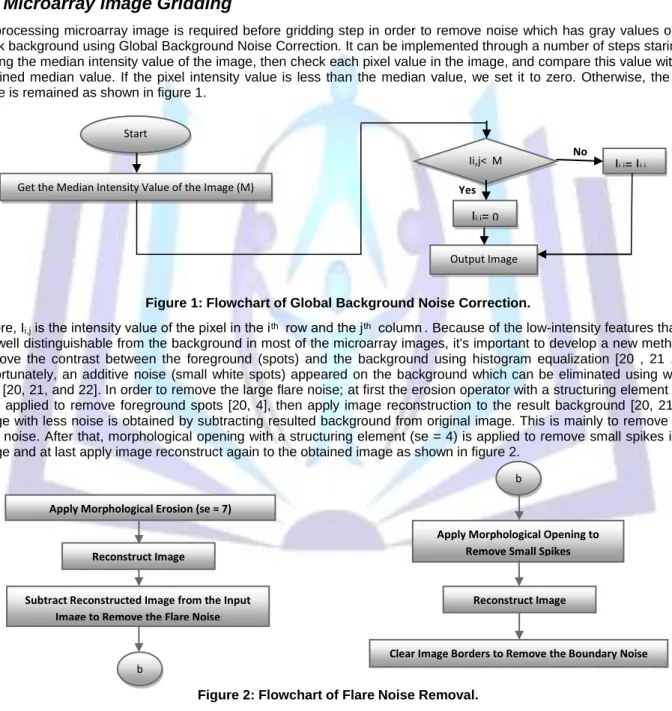
Preprocessing microarray image is required before gridding step in order to remove noise which has gray values on the black background using Global Background Noise Correction. It can be implemented through a number of steps staring by getting the median intensity value of the image, then check each pixel value in the image, and compare this value with the obtained median value. If the pixel intensity value is less than the median value, we set it to zero. Otherwise, the pixel value is remained as shown in figure 1.
Figure 1: Flowchart of Global Background Noise Correction.
Where, Ii,j is the intensity value of the pixel in the i ͭ ͪ row and the j ͭ ͪ column . Because of the low-intensity features that are
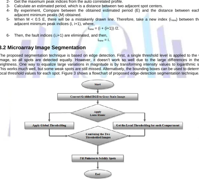
not well distinguishable from the background in most of the microarray images, it's important to develop a new method to improve the contrast between the foreground (spots) and the background using histogram equalization [20 , 21 , 22]. Unfortunately, an additive noise (small white spots) appeared on the background which can be eliminated using wiener filter [20, 21, and 22]. In order to remove the large flare noise; at first the erosion operator with a structuring element (se = 7) is applied to remove foreground spots [20, 4], then apply image reconstruction to the result background [20, 21]. An image with less noise is obtained by subtracting resulted background from original image. This is mainly to remove large flare noise. After that, morphological opening with a structuring element (se = 4) is applied to remove small spikes in the image and at last apply image reconstruct again to the obtained image as shown in figure 2.
Figure 2: Flowchart of Flare Noise Removal.
The Projection Profile Method is then applied to the binary image obtained using canny edge detection operator [23, 24]. Then, the detected spots are filled using region filling operation. Despite canny detector is one of the best edge detectors that suppresses noise, it couldn't detect some spots well in the image, as it produces some incomplete regions which is difficult to be filled. To overcome this problem; morphological opening (erosion then dilation) is applied on the resulted binary image [4]. In order to obtain the horizontal intensity projection profile H P(y) of the image [25] f(x,y), the sum of intensity values are calculated at each pixel along the x-axis for each row, which is defined as follow:
Yes
No Start
Ii,j< M Ii,j= Ii,j
Ii,j= 0 Get the Median Intensity Value of the Image (M)
Output Image
Apply Morphological Erosion (se = 7)
Reconstruct Image
Subtract Reconstructed Image from the Input Image to Remove the Flare Noise
Apply Morphological Opening to Remove Small Spikes
Reconstruct Image
Clear Image Borders to Remove the Boundary Noise b
𝑃(𝑦) = 𝑥=𝑥−1𝑥=0 f (x, y)(1)
Where,image size is X × Y, HP(y) represents the horizontal projection signal. The negative peaks of the profile are detected that correspond to the positions of the vertical grid lines. The actual image contains noise and other factors, so if directly use the above method for gridding, it may cause the phenomenon of missing or redundant grid lines. Therefore, to grid the image correctly, de-noising and refinement of the projection profile is required.
Finally, to determine the horizontal grid lines, the image matrix is transposed for only one time, and then repea=the previous steps starting from obtaining the projection profile. After all these steps it is found that There is a need to apply the Post- Processing Technique as there're a lot of sharp spikes may be appeared on the image profiles, that is treated as that false peaks. So, before performing the computations, a new approach is proposed to enhance and de-noise the calculated profile by applying two filters: un-sharpening and smoothing. The smoothing filter size value was set to 7 according to the experiment. The proposed method has high accuracy, but in practice, no methods can grid entirely correct. Therefore, a grid correction or refinement method is developed through the following steps:
1- Apply autocorrelation to the mean horizontal profile [20 , 25], where, autocorrelation [26] is the cross-correlation of a signal with itself.
2- Get the maximum peak indices from the auto correlated profile.
3- Calculate an estimated period, which is a distance between two adjacent spot centers.
4- By experiment, Compare between the obtained estimated period (E) and the distance between each two adjacent minimum peaks (M) obtained.
5- When M < 0.5 E, there will be a mistakenly drawn line. Therefore, take a new index (inew) between the two
adjacent minimum peak indices (i, i+1), where,
inew = (i + (i+1)) /2.
6- Then, the fault indices (i,i+1) are eliminated, and then, inew = i.
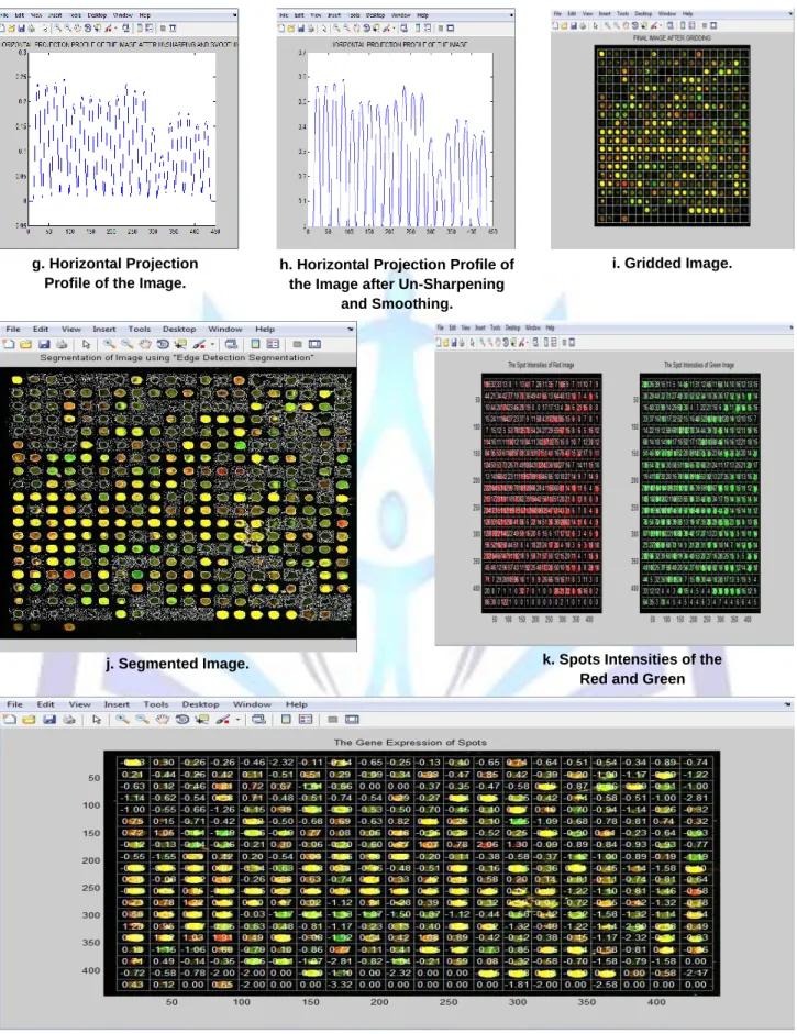
3.2 Microarray Image Segmentation
The proposed segmentation technique is based on edge detection. First, a single threshold level is applied to the whole image, so all spots are detected equally. However, it doesn‟t work so well due to the large differences in the spot brightness. One way to equalize large variations in magnitude is by transforming intensity values to logarithmic space. This works much well, but some weak spots are still missed. Alternatively, the bounding boxes can be used to determine local threshold values for each spot. Figure 3 shows a flowchart of proposed edge-detection segmentation technique.
Figure 3: Flowchart of Edge-Detection Segmentation Technique.
Unfortunately, results reveal that weak spots showed up well but spots with bright perimeters were as bad as the original global threshold before log space transformation. Since each of the local and the global thresholding has a special advantage, the best of both approaches are combined by apply „ORing‟ to the two thresholded images. The results were indeed much better. The silhouettes of some spots still contained pinholes. The whole image could be filled using image filling operation, but this may not be a good idea as some spots run together. If four mutually adjacent spots (sharing a common corner) are all joined at their edges then a single function call would incorrectly fill in the common corner as well. To avoid that possibility, it is safer to fill each spot; take each bounding box region at a time by looping.
3.3 Microarray Image Quantification
In the quantification step, each segmented spot in its corresponding bounding box region is extracted at a time by looping, to measure its red and green intensities, and ultimately quantify its gene expression value. The purpose of the spot quantification is to combine intensity values of the red and green components into a unique quantitative measure that can be used to represent the expression level of gene deposited in a given spot [2]. The nominal intensity over the spot for both the red and green layers is calculated. A measure of gene expression level can then be calculated from the two color intensities. It is common practice to transform DNA microarray data from the raw intensities into log intensities (base2) before proceeding further analysis [2 , 27].There are several objectives for this transformation such as (i) there should a reasonably even spread of features across the intensity range, (ii) the variability should be constant all intensity levels, (iii) the distribution of experimental errors should be normal, (iv) the distribution of intensity should be approximately bell shaped. Here a 2 fold up regulated genes corresponds to a log ratio of +1 and 2 fold down regulated genes correspond to a log ratio of -1. Genes that are not differentially expressed have a log ratio of 0. Log differential ratio (expression ratio) is usually denoted by (M).Gene Expression Level (M) = Log (Intensity (Red) (R) / Intensity (Green) (G)) (2)
4. RESULTS AND DISCUSSION
The proposed analysis method of cDNA microarray images is implemented on a number of noisy microarray images from the Stanford Microarray Database (SMD). The cropped microarray image is composed of the same number of rows and columns of spots. Depending on the degree of noise and how the spots are expressed, two types of images are used:
1- High quality (good image). 2- Low quality images (Bad image).
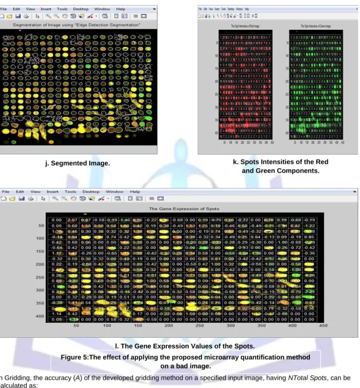
The following two figures show the detailed steps and the results of applying the proposed method on two types of images having different qualities. Figure 4 shows the effect of applying the proposed microarray quantification method on a good image and figure 5 shows the effect of applying the proposed microarray quantification method on a bad image.
4.1 Good Image
a. Original Image. b. Gray Scale Image. c. Image after Removing Background Noise.
d. Image after Removing Additive Noise.
e. Image after Removing Flare Noise.
f. Image after Applying Canny, Filling, and Opening Operations.
g. Horizontal Projection Profile of the Image.
h. Horizontal Projection Profile of the Image after Un-Sharpening
and Smoothing.
i. Gridded Image.
j. Segmented Image. k. Spots Intensities of the Red and Green
Components.
l. The Gene Expression Values of the Spots.
Figure 4:The effect of applying the proposed microarray quantification method on a good image.
4.2 Bad Image
a. Original Image. b. Gray Scale Image. c. Image after Removing Background Noise.
e. Image after Removing Flare Noise.
f. Image after Applying Canny, Filling, and Opening Operations. d. Image after Removing
Additive Noise.
h. Horizontal Projection Profile of the Image after Un-Sharpening
and Smoothing.
i. Gridded Image. g. Horizontal Projection
In Gridding, the accuracy (A) of the developed gridding method on a specified input image, having NTotal Spots, can be calculated as:
A = (NCorrect Spots / NTotal Spots) *100 %. (2)
Where, NCorrect Spots, NTotal Spotsindicates the number of spots correctly gridded and the total number of spots in the image respectively.
Table 1. Summary of Gridding Results
TYPE OF IMAGE ACCURACY
Good 100%
Bad 96.2%
j. Segmented Image. k. Spots Intensities of the Red and Green Components.
l. The Gene Expression Values of the Spots.
Figure 5:The effect of applying the proposed microarray quantification method on a bad image.
As shown in table 1, the proposed gridding method has high griddingaccuracy values. By comparing the proposed gridding method to other existing methods as those implemented by Deepa J and Tessamma Thomas [28], BasimAlhadidi [29], and Fatma El-ZahraaLabib [30], it was found that the proposed method is more accurate and can grid various types of noisy images correctly as it mainly deals with noisy images. In practice, no method can grid entirely correct. Therefore, pre-processing, post-processing, and refinement steps used in this work can effectively enhance the contrast and eliminate various kinds of noise in the image. This applicable method can correctly grid the two kinds of noisy microarray images selected in this paper as a sample without any human intervention.
The second basic step for analyzing the cDNA microarray noisy images is segmentation. The edge-detection segmentation method used in this work can segment the previously gridded microarray images correctly with high accuracy results. Figure 4 (j) and Figure 5 (j) show the resulting images after applying the edge-detection step. Both global and local thresholding of the logarithmic image are applied, and then the two images are combined to get the advantage of each of them. When global and the local thresholdingare appliedon the gray scale image rather than the logarithmic one, it gives results with less accuracy and some data become undistinguishable as well.
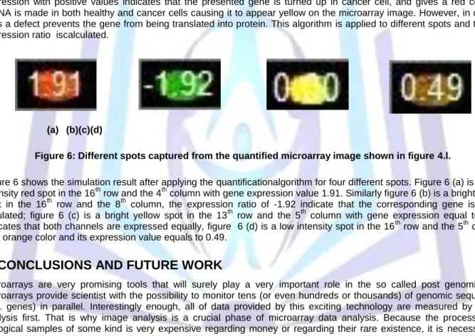
To achieve the quantification step, the intensity for each spot is calculated in both the red and green components of the image. Then the gene expression values or the amount of hybridization on each spot is calculated by applying the logarithmic equation, and by the usage of the obtained intensity values from both components. It‟s obviously shown from the above figures that the gene expression with negative values indicates that the presented gene didn‟t change and works properly in the cancer tissue. Thus, it gives a green color. This gene is not in the researcher‟s interest. The gene expression with positive values indicates that the presented gene is turned up in cancer cell, and gives a red color. If mRNA is made in both healthy and cancer cells causing it to appear yellow on the microarray image. However, in cancer cells a defect prevents the gene from being translated into protein. This algorithm is applied to different spots and the log expression ratio iscalculated.
(a) (b)(c)(d)
Figure 6: Different spots captured from the quantified microarray image shown in figure 4.l.
Figure 6 shows the simulation result after applying the quantificationalgorithm for four different spots. Figure 6 (a) is a high intensity red spot in the 16th row and the 4th column with gene expression value 1.91. Similarly figure 6 (b) is a bright green spot in the 16th row and the 8th column, the expression ratio of -1.92 indicate that the corresponding gene is down regulated; figure 6 (c) is a bright yellow spot in the 13th row and the 5th column with gene expression equal to 0.00 indicates that both channels are expressed equally, figure 6 (d) is a low intensity spot in the 16th row and the 5th column with orange color and its expression value equals to 0.49.
5. CONCLUSIONS AND FUTURE WORK
Microarrays are very promising tools that will surely play a very important role in the so called post genomic era. Microarrays provide scientist with the possibility to monitor tens (or even hundreds or thousands) of genomic sequences (e.g. genes) in parallel. Interestingly enough, all of data provided by this exciting technology are measured by image analysis first. That is why image analysis is a crucial phase of microarray data analysis. Because the processing of biological samples of some kind is very expensive regarding money or regarding their rare existence, it is necessary to decrease the human interaction as much as possible, as this disables complete repeatability of the analysis. In this paper, the three basic steps for processing the cDNA microarray images were developed; gridding, segmentation, and quantification. Two kinds of microarray images with different degree of noise were selected to test the proposed method. First, a gridding technique was applied which gives good results with accuracy ranges from 96.2% - 100%. The segmentation technique based on “edge detection” was presented with high accuracy. Finally, the proposed quantification technique was applied by calculating the intensity value of each spot in the red and green components of an image, to get the gene expression values. The future work intended to pursue the research for developing new algorithms of gridding, extracting the spot from the background, enhance the microarray image and calculating the intensity for each spot. Also the work done is to be realized in the future through integration with the hardware and experiments.
REFERENCES
[1] Brown P.O. and Botstein D. , “ Exploring the new world of genome with microarrays” , Nature Genetics, vol.21, pp
33-37,1999.
[2] Sorin, Draghici, Data analysis tool for DNA Microarrays, Chapman&Hall/CRC, Mathematical biology and medicine series, London NewYork, 2003.
[3] Istepanian, R., Microarray image processing: Current status and future directions. IEEE Tran. Nanobioscience, 2: 4, 2003.
[4] Y. Wang, F. Y. Shih, and M. Ma, “Precise gridding of microarray images by detecting and correcting rotations in
sub-arrays'' in proceedings of Sixth Inter. Conf. on Computer Vision, Pattern Recognition and Image Processing, Salt Lake City, UT, July 2005.
[5] T. Tu et al., “Quantitative noise analysis for gene expression microarray experiments”, Proc. Natl. Acad. Sci., 99,
14031-6, 2002.
[6] G. Antoniol and M. Ceccarelli, “A Markov Random Field Approach to Microarray Image Gridding,” Proc. 17thInt‟l
Conf.Pattern Recognition,pp.550-553,2004.
[7] J.Buhler, T.Ideker and D.Haynor, “Dapple: Improved Techniques for Findings Spots on DNA Microarrays” . Technical
ReportUWTR 2000-08-05, University of Washington,2000.
[8] A.Jain, T.Tokuyasu, A.Snijderts, R.Segraves, D.Albertson and D.Pinkel, “Fully Automatic Quantification of Microarray
Image Data”, Genome Res., 12(2):325 – 332, 2003.
[9] P. Arena, M. Bucolo, L. Fortuna, and L. Occhipinty, Cellular neural networks for real-time DNA microarray analysis, IEEE Eng Med Bio 21 (2002), 17-25.
[10] X. Y. Zhang, F. Chen, Y. T. Zhang, S. G. Agner, M. Akay, Z. H. Lu, M. M. Y. Waye, and S. K. W. Tsui, Signal Processing techniques in genomic engineering, Proc IEEE 90 (2002), 1822-1833.
[11] A. P. G. Damiance, L. Zhao, and A. C. P. L. F. Carvalho, A dynamic model with adaptive pixel moving for microarray images segmentation, Real-Time Imaging 10 (2004), 189-195.
[12] M. Katzer, F. Kummert, and G. Sagerer, Methods for automatic microarray image segmentation, IEEE Trans Nanobiosci 2 (2003), 202-213.
[13] R. Hirata Jr, J. Barrera, R. F. Hashimoto, D. O. Dantas, and G. H. Esteves, Segmentation of microarray images by mathematical morphology, Real-Time Imaging 8 (2002), 491-505.
[14] R. Nagarajan, Intensity-based segmentation of microarrays images, IEEE Trans Med Imaging 22 (2003), 882-889.
[15] A. W. C. Liew, H. Yana, and M. Yang, Robust adaptive spot segmentation of DNA microarray images, Pattern Recognit 36 (2003), 1251-1254.
[16] Y. H. Yang, M. J. Buckley, S. Dudoit, and T. P. Speed, Comparison of methods for image analysis on cDNA microarray data, J Comput Graph Stat 11 (2002), 108-136.
[17] Y. Chen, E. Dougherty, and M. Bittner, Ratio-based decisions and the quantitative analysis of cDNA microarray images, J Biomed Opt 2 (1997), 364-374.
[18] Islam A. Fouad, Mai S. Mabrouk, and Amr A. Sharawy, A new method to grid noisy cDNA microarray images utilizing denoising techniques, International Journal of Computer Applications (0975 – 8887), 63(9), 2013.
[19] Islam Abdul-AzeemFouad, FatmaZahraa Mohamed Labib, Mai Said Mabrouk, and Amr Abdel RahmanSharawy, Developing a new methodology for de-noising and gridding cDNA microarray images, 2012 6th Cairo International Biomedical Engineering Conference, Cairo, Egypt, 2012.
[20] Matlab (R2012b) Image Processing Toolbox, Signal Processing Toolbox.
[21] Rafael C. Gonzalez and Richard E.Woods,“Digital Image processing”, Second Edition.
[22] AcharyaTinku, Ray Ajoy K., “Image Processing Principles and Applications”. John Wiley & Sons, Inc. (2005).
[23] J.F. Canny, “A computational approach to edge detection,” IEEE Trans Pattern Analysis and Machine Intelligence,
vol. 8, no. 6, pp. 679-698, Nov. 1986.
[24] Li Qin, Luis Rueda, Adnan Ali and AliouneNgon, “Spot Detection and Image Segmentation in DNA Microarray Data”, Appl. Bioinformatics. 2005;4(1):1-11.
[25] J.Angulo and J.Serra, “Automatic analysis of DNA microarray images using mathematical morphology”,
Bioinformatics, vol.19,no.5,pp.553-562,2003.
[26] Internet, http://en.wikipedia.org/wiki/Autocorrelation.
[27] Dov S, ―Microarray Bioinformatic”s, Cambridge University Press, Newyork, 2003.
[28] Deepa J, and Tessamma Thomas, “Automatic Gridding of DNA Microarray Images using Optimum Subimage”, International Journal of Recent Trends in Engineering, Vol. 1, No. 4, May 2009.
[29] BasimAlhadidi, HussamNawwafFakhouri and Omar S. AIMousa, “cDNA Microarray Genome Image Processing Using Fixed Spot Position”, American Journal of Applied Science 3(2): 17301734, 2006.
[30] Fatma El-ZahraaLabib, Islam Fouad, Mai Mabrouk, and AmrSharawy, An efficient fully automated method for gridding microarray images, American Journal of Biomedical Engineering, 2(3), 115-119, 2012.
Islam A. Fouad
Islam Abdul-AzeemFouad received his BSc in Systems and Biomedical Engineering Department, Cairo University, Giza, Egypt, in 2001. He completed his MSc in Biomedical Engineering from the same school in 2006. He is a Lecturer in Biomedical Technology Department, Salman bin Abdul-Aziz University, since September 2009. He has several research papers in the area of image processing and bioinformatics. His research interests include biomedical image processing and bioinformatics in addition to brain computer interface(BCI).
Mai S. Mabrouk
Mai Said Mabrouk received her BSc in Systems and Biomedical Engineering Department, CairoUniversity, Giza, Egypt, in2000. She completed her MSc and PhD in Biomedical Engineering from thesame school in 2004 and 2008, respectively. She is an Assistant Professor with the BiomedicalEngineering Department, Misr University for Science and Technology (MUST), since August 2008. Shehas several research papers in the area of image processing and bioinformatics. Her research interestsinclude biomedical image processing, bioinformatics and digital signal processing in addition to genomicsignal processing.
Amr A. Sharawi
Amr A. Sharawi, PhD, Systems and Biomedical Engineering Department, Faculty of Engineering, CairoUniversity, P.O.B. 12211, Giza, Egypt ([email protected]). Amr A. Sharawi, PhD, is with CairoUniversity. He received his BS degree inElectronics and Communication in 1976 from Cairo University.He received his MS degree in Systems and Biomedical Engineering in 1981from Cairo University.Furthermore, he received his PhD degree in Systems and Biomedical Engineering in July 1991. Since2001, he has been an associate professor in biomedical engineering at Cairo University, Faculty ofEngineering. His research interests include mainly clinical engineering, bioinformatics and medicalimaging.