October 2009, Volume 32, Issue 1. http://www.jstatsoft.org/
Effect Displays in
R
for Multinomial and
Proportional-Odds Logit Models:
Extensions to the
effects
Package
John Fox McMaster University
Jangman Hong McMaster University
Abstract
Based on recent work by Fox and Andersen (2006), this paper describes substantial extensions to the effects package forR to construct effect displays for multinomial and proportional-odds logit models. The package previously was limited to linear and gener-alized linear models. Effect displays are tabular and graphical representations of terms – typically high-order terms – in a statistical model. For polytomous logit models, effect displays depict fitted category probabilities under the model, and can include point-wise confidence envelopes for the effects. The construction of effect displays by functions in the
effects package is essentially automatic. The package provides several kinds of displays for polytomous logit models.
Keywords: effect displays, multinomial logit model, proportional-odds model, statistical graph-ics, R.
An “effect display” is a table or graph meant to represent a term in a statistical model. Effect displays are generalizations of similar methods, such as Fisher’s (1936) “adjusted means” in the analysis of covariance,Goodnight and Harvey’s (1978) “least-squares means” in analysis of variance and covariance, and Searle, Speed, and Milliken’s (1980) “estimated population marginal means.” To create an effect display, predictors in a term are allowed to range over their combinations of values, while other predictors in the model are held to “typical” values. The primary motivation for effect displays is the difficulty of interpreting many statistical models directly from their estimated coefficients. For example, to interpret a linear model with interactions requires that main effects – and possibly lower-order interactions – marginal to an interaction be combined with the interaction, an operation that can entail mental gymnastics. Similarly, the coefficients of regression splines defy direct interpretation. These difficulties are compounded in generalized linear models, where interest usually inheres more directly in the scale of the response variable than in the scale of the linear predictor on which
the coefficients of the model are expressed.
Effect displays for generalized linear models were introduced by Fox (1987), and an imple-mentation in the effects package for the statistical programming environment R (Ihaka and
Gentleman 1996;RDevelopment Core Team 2009) was described in Fox (2003). The
multi-nomial and proportional-odds logit models are common statistical models for polytomous (i.e., multi-category) categorical responses; these models are described in many sources (see, e.g., Fox 2008, Section 14.2). Fox and Andersen (2006) extended effect displays to multi-nomial and proportional-odds logit models where the principal obstacle was the derivation of standard errors for the effects. Fox and Andersen’s results are given in Appendix A, which describes the extension of the effects package to multinomial and proportional-odds logit models. The package is available from the ComprehensiveRArchive Network athttp: //CRAN.R-project.org/package=effects.
1. Review of effect displays for generalized linear models
The computation of effect displays is particularly simple for a generalized linear model, with linear predictor η = Xβ and link function g(µ) = η; here, µ is the expectation of the response vector y. Let βb represent an estimate of β, and Vb(bβ) the estimated covariance matrix ofβb. Let the rows ofX0 include all combinations of values of predictors appearing in a high-order term of the model, along with typical values of the remaining predictors. The structure ofX0, with respect for example to contrasts and interactions, is identical to that ofthe model matrixX. We compute fitted valuesηb0=X0βb to represent the term in question, consequently absorbing terms marginal to it. An “effect display” is a graph of these fitted values as a function of the predictors in the term, or of the fitted values transformed to the scale of the response, g−1(ηb0). The standard errors of ηb0, the square-root diagonal entries of X0V(b βb)X
0
0, may be used to compute point-wise confidence intervals for the effects; the
end-points of these confidence intervals may also be transformed to the scale of the response. To illustrate effect displays for a generalized linear model, we develop a logistic-regression model for the Titanic data set in the effects package. This data set contains information about the survival status, sex, age, and passenger class of 1309 passengers on the ill-fated 1912 maiden voyage of the ocean linerTitanic:
R> library("effects")
Loading required package: lattice Loading required package: grid Loading required package: MASS Loading required package: nnet
Loading required package: colorspace Attaching package: 'effects'
The following object(s) are masked from package:datasets : Titanic
R> summary(Titanic)
survived sex age passengerClass no :809 female:466 Min. : 0.1667 1st:323
yes:500 male :843 1st Qu.: 21.0000 2nd:277 Median : 28.0000 3rd:709 Mean : 29.8811
3rd Qu.: 39.0000 Max. : 80.0000 NA's :263.0000
Notice that the variable age is missing for 263 passengers. In the analysis reported below, we simply omit observations with missing age; for a more careful analysis of the Titanic data, including imputation of missing data, see Harrell (2001, Chapter 12). The command example(Titanic)reproduces the results that we present in this section.
We begin with a logistic regression of survival on sex, age, and passenger class, including all interactions among the three predictors:
R> library("car")
R> titanic.1 <- glm(survived ~ passengerClass * sex * age, data = Titanic,
+ family = binomial)
R> Anova(titanic.1)
Anova Table (Type II tests) Response: survived LR Chisq Df Pr(>Chisq) passengerClass 121.519 2 < 2.2e-16 *** sex 275.779 1 < 2.2e-16 *** age 34.913 1 3.447e-09 *** passengerClass:sex 38.161 2 5.171e-09 *** passengerClass:age 10.061 2 0.006537 ** sex:age 4.331 1 0.037429 * passengerClass:sex:age 1.866 2 0.393344 ---Signif. codes: 0 '***' 0.001 '**' 0.01 '*' 0.05 '.' 0.1 ' ' 1
Thus, the three-way interaction among the predictors is non-significant, but each of the two-way interactions is statistically significant. We proceed to remove the three-two-way interaction and refit the model:
R> titanic.2 <- update(titanic.1, . ~ . - passengerClass:sex:age)
R> summary(titanic.2)
Call:
passengerClass:age + sex:age, family = binomial, data = Titanic) Deviance Residuals:
Min 1Q Median 3Q Max
-2.6138 -0.6755 -0.4435 0.3772 3.2448 Coefficients:
Estimate Std. Error z value Pr(>|z|) (Intercept) 3.390355 0.805280 4.210 2.55e-05 *** passengerClass2nd 0.764667 0.959843 0.797 0.425650 passengerClass3rd -3.270002 0.764823 -4.276 1.91e-05 *** sexmale -2.592233 0.753573 -3.440 0.000582 *** age -0.003950 0.017574 -0.225 0.822158 passengerClass2nd:sexmale -0.878841 0.689942 -1.274 0.202738 passengerClass3rd:sexmale 1.885695 0.584625 3.225 0.001258 ** passengerClass2nd:age -0.060530 0.021420 -2.826 0.004714 ** passengerClass3rd:age -0.006244 0.016188 -0.386 0.699711 sexmale:age -0.031378 0.015117 -2.076 0.037929 * ---Signif. codes: 0 '***' 0.001 '**' 0.01 '*' 0.05 '.' 0.1 ' ' 1 (Dispersion parameter for binomial family taken to be 1)
Null deviance: 1414.62 on 1045 degrees of freedom Residual deviance: 917.84 on 1036 degrees of freedom
(263 observations deleted due to missingness) AIC: 937.84
Number of Fisher Scoring iterations: 5
TheallEffects function in the effects package will compute effects for all high-order terms in a model – that is, terms that are not marginal to any others in the model:
R> titanic.2.all <- allEffects(titanic.2, typical = median, given.values =
+ c(passengerClass2nd = 1/3, passengerClass3rd = 1/3, sexmale = 0.5))
R> print(titanic.2.all, digits = 3)
model: survived ~ passengerClass + sex + age + passengerClass:sex + passengerClass:age + sex:age
passengerClass*sex effect sex
passengerClass female male 1st 0.964 0.452 2nd 0.913 0.119 3rd 0.459 0.148
passengerClass*age effect age passengerClass 0.166700006 9.037066672 17.907433338 26.777800004 35.64816667 1st 0.890 0.872 0.851 0.828 0.801 2nd 0.917 0.845 0.728 0.568 0.392 3rd 0.441 0.385 0.333 0.284 0.239 age passengerClass 44.518533336 53.388900002 62.259266668 71.129633334 80 1st 0.772 0.740 0.705 0.6676 0.6279 2nd 0.241 0.135 0.071 0.0362 0.0181 3rd 0.200 0.166 0.137 0.1117 0.0908 sex*age effect age sex 0.166700006 9.037066672 17.907433338 26.777800004 35.64816667 female 0.928 0.910 0.890 0.865 0.835 male 0.572 0.445 0.325 0.224 0.148 age sex 44.518533336 53.388900002 62.259266668 71.129633334 80 female 0.800 0.7606 0.716 0.6662 0.6127 male 0.094 0.0586 0.036 0.0219 0.0133
By default, theeffect function, whichallEffectscalls, sets covariates – in this case, age is the only covariate – not included in a term to their mean values; factors are set to their pro-portional distribution in the data by averaging over contrasts. In the call to allEffects, we overrode these defaults, specifyingtypical = medianto compute the median rather than the mean of excluded covariates, and setting given.values = c(passengerClass2nd = 1/3, passengerClass3rd = 1/3, sexmale = 0.5) to fix the distribution of passenger class to 1/3 in each level and the distribution of sex to half male and half female. Also by default, effectsets age to 10 values evenly spaced over its range; we can optionally supply the number of values for a covariate via thedefault.levels argument or we can set the values directly, as illustrated below. Notice that the print method for the object returned by allEffects reports tables of the effects, which, by default, are on the scale of the response variable – for a logit model, on the probability scale. There is also asummarymethod (not employed here), which provides greater detail.
To plot the effects on one page (producing Figure1):
R> plot(titanic.2.all, ticks =
+ list(at = c(.01, .05, seq(.1, .9, by = .2), .95, .99)), ask = FALSE)
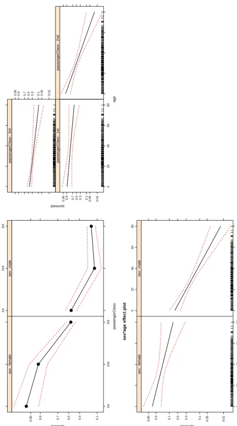
The default is to plot on the scale of the linear predictor, where the linearity of the model is preserved, but to label the response axis on the generally more easily interpreted scale of the response. Because the plotted effects span a wider range on the probability scale than is accommodated by the default tick marks, we specify custom tick marks via the ticks argument; setting ask = FALSEproduces a multi-panel display of all of the high-order terms in the model. The broken lines on the graphs represent point-wise 95-percent confidence envelopes around the fitted values, and the panels showing age give the marginal distribution of age in the “rug-plot” at the bottom of the graphs.
passengerClass*sex effect plot passengerClass survived 0.1 0.3 0.5 0.7 0.9 0.95 1st 2nd 3rd ● ● ● : sex female 1st 2nd 3rd ● ● ● : sex male
passengerClass*age effect plot
age survived 0.05 0.01 0.1 0.3 0.5 0.7 0.9 0.95 0 20 40 60 80 : passengerClass 1st : passengerClass 2nd 0.01 0.05 0.1 0.3 0.5 0.7 0.9 0.95 : passengerClass 3rd
sex*age effect plot
age survived 0.05 0.01 0.1 0.3 0.5 0.7 0.9 0.95 0 20 40 60 80 : sex female 0 20 40 60 80 : sex male
Figure 1: Effect display for high-order terms in the binary logistic-regression model fit to the Titanic data. The red broken lines give point-wise 95-percent confidence envelopes around the fitted effects.
The panel at the top left of Figure 1 displays the passenger-class × sex interaction: For fe-male passengers, survival decreased with class, while for fe-male passengers, survival was highest for first-class passengers but essentially the same for second- and third-class passengers. Fe-male third-class passengers had approximately the same level of survival as Fe-male first-class passengers.
The top-right panel depicts the class-by-age interaction: Survival declined with age for all three passenger classes, but most dramatically for second-class passengers. First-class pas-sengers had quite a high level of survival, and third-class paspas-sengers a relatively low level of survival, at all ages.
The lower-left panel shows the sex-by-age interaction: For both sexes, survival decreased with age, but age made more of a difference for males than for females, and the youngest males survived at approximately the same rate as the oldest females.
The 95-percent point-wise confidence envelopes suggest that all of the effects are reasonably precisely estimated (on the probability scale, which is expanded at the extremes of the logit scale), except at the highest ages.
Although these graphs of the two-way interactions are more easily interpreted than the coeffi-cients of the logit model, combining three “overlapping” two-interactions nevertheless requires visual contortions. The effect function allows us to combine the two-way interactions by plotting the absent three-way interaction to which they are marginal (see Figure 2), a proce-dure that generates a warning:
R> with(Titanic, quantile(age, c(0, 0.99), na.rm = TRUE))
0% 99% 0.1667 65.0000
R> plot(effect("passengerClass*sex*age", titanic.2, xlevels =
+ list(age = 0:65)), ticks = list(at = c(.001, .005, .01, .05,
+ seq(.1, .9, by = .2), .95, .99, .995)))
Warning message:
In analyze.model(term, mod, xlevels, default.levels) : passengerClass:sex:age does not appear in the model
As before, we supply custom tick marks, and we restrict age, which is highly skewed, to run from 0 to its 99th percentile, via the argumentxlevels = list(age = 0:65)). We can spec-ify the three-way interaction as either "passengerClass*sex*age" or "passengerClass:sex:age", but the order of the predictors must be the same as in the model.
The display in Figure2is, we maintain, easier to digest than the separate panels for the three two-way interactions shown in Figure1, but the general pattern of the results is as we have described above. A reasonable brief summary is that survival on the Titanic was of “women and children first,” but modified by passenger class.
Because the model fit to the data is linear in age on the logit scale, it is possible to arrive at these conclusions by examining the estimated coefficients of the model, but to do so requires
passengerClass*sex*age effect plot age survived 0.001 0.0050.01 0.050.1 0.3 0.5 0.7 0.9 0.95 0.99 0.995 0 20 40 60 : passengerClass 1st : sex female : passengerClass 2nd : sex female 0 20 40 60 : passengerClass 3rd : sex female : passengerClass 1st : sex male 0 20 40 60 : passengerClass 2nd : sex male 0.001 0.005 0.01 0.05 0.1 0.3 0.5 0.7 0.9 0.95 0.99 0.995 : passengerClass 3rd : sex male
Figure 2: Effect display for the three-way interactionpassengerClass×sex ×age, a term that is not in the model fit to the Titanic data, but to which all of the two-way interactions in the model are marginal.
laboriously adding terms according to relationships of marginality among them, a process that is automated in the effect displays. Moreover, the effect plots in Figures 1 and 2 label axes on the more easily interpreted probability scale.
2. Effect displays for multinomial logit models
The multinomial logit model is probably the most common regression model for polytomous categorical data. Theeffectspackage uses the implementation of the multinomial logit model in themultinomfunction from the nnetpackage (associated withVenables and Ripley 2002), one of the “recommended” packages that ship with standardRdistributions.
The multinomial logit model takes the following form: µij = exp(x0iβj) 1 + m P k=2 exp(x0kβj) forj= 2, ..., m (1) µi1= 1 1 + m P k=2 exp(x0kβj) (for level 1) = 1− m X k=2 µik
Here,µij is the probability that the response variable is in itsjth ofm levels for observation i; x0i is the ith row of the model matrix X; and βj is a vector of p regression coefficients pertaining to level j of the response. The first level of the response is treated specially to insure that
m P j=1
µij = 1; this choice is arbitrary and inconsequential, in the sense that the model produces the same set of fitted probabilities regardless of the response level singled out for special treatment. The interpretation of the regression coefficients, however, depends upon the selection of “baseline” level for the response, because
logµij µi1
=x0iβj forj= 2, ..., m
Thus, the coefficients represent effects on the log-odds of membership in levelj versus level 1 of the response. Differences in coefficients give effects on the log-odds of membership in other pairs:
log µij µij0 =x
0
i(βj−βj0) forj, j0 6= 1
Producing effect displays on the probability scale for the multinomial logit model is relatively straightforward, because the model yields fitted probabilitiesbµ0j for specified values of the lin-ear predictorsx00βbj. The only difficult point is the calculation of standard errors for the effects. We adopt the strategy of displaying effects on the probability scale, but computing standard errors and confidence intervals on the scale of the individual-level logits, log [µ0j/(1−µ0j)]: Because the probabilities are bounded by 0 and 1, while the logits are unbounded, confidence intervals on the logit scale are better-behaved. We outline this procedure in the AppendixA; a more extended treatment may be found in Fox and Andersen(2006).
The data frameBEPSin theeffectspackage contains data from the 1997-2001 British Election Panel Study. We adapt an example that appeared in Fox and Andersen (2006), which, in turn, was based on work by Andersen, Heath, and Sinnott(2002). The focus of the example (available via the command example(BEPS)) is the interaction between political knowledge and electoral choice: Individuals who are familiar with political parties’ platforms are expected to be more likely to align their votes with their preferred positions on issues, in this case, with the issue of the UK’s integration into the European Union. The data set contains the following variables:
vote age economic.cond.national Conservative :462 Min. :24.00 Min. :1.000
Labour :720 1st Qu.:41.00 1st Qu.:3.000 Liberal Democrat:343 Median :53.00 Median :3.000 Mean :54.18 Mean :3.246 3rd Qu.:67.00 3rd Qu.:4.000 Max. :93.00 Max. :5.000
economic.cond.household Blair Hague Kennedy Min. :1.000 Min. :1.000 Min. :1.000 Min. :1.000 1st Qu.:3.000 1st Qu.:2.000 1st Qu.:2.000 1st Qu.:2.000 Median :3.000 Median :4.000 Median :2.000 Median :3.000 Mean :3.140 Mean :3.334 Mean :2.747 Mean :3.135 3rd Qu.:4.000 3rd Qu.:4.000 3rd Qu.:4.000 3rd Qu.:4.000 Max. :5.000 Max. :5.000 Max. :5.000 Max. :5.000
Europe political.knowledge gender Min. : 1.000 Min. :0.000 female:812 1st Qu.: 4.000 1st Qu.:0.000 male :713 Median : 6.000 Median :2.000
Mean : 6.729 Mean :1.542 3rd Qu.:10.000 3rd Qu.:2.000 Max. :11.000 Max. :3.000
voteis a factor with three levels, Conservative,Labour, andLiberal Democrat. The Conservatives were generally opposed to increased UK participation in the EU, while the other two parties adopted a pro-Europe position.
Europe is an 11-point scale measuring the respondent’s attitudes towards European integration, with high scores representing “Eurosceptic” (i.e., anti-EU) sentiment.
political.knowledge assesses the respondent’s familiarity with the parties’ positions on the European-integration issue. Scores range from 0 (representing knowledge of none of the parties’ positions) to 3 (knowledge of all three positions).
Age, gender, perceptions of economic conditions over the past year (both national and household), and evaluations of the leaders of the three major parties are included in the model as “control variables” because of their known relationship to voting.
After exploration of the data, we model Europe as a three-degree-of-freedom regression spline. (Fox and Andersen 2006, employed a simpler model in which both Europe and political.knowledgeentered the model linearly.)
R> library("splines")
R> beps <- multinom(vote ~ age + gender + economic.cond.national +
+ economic.cond.household + Blair + Hague + Kennedy +
+ bs(Europe, 3) * political.knowledge, data = BEPS)
# weights: 48 (30 variable) initial value 1675.383740
iter 10 value 1180.708452 iter 20 value 1118.628662 iter 30 value 1099.897721 final value 1099.705647 converged R> summary(beps) Call:
multinom(formula = vote ~ age + gender + economic.cond.national + economic.cond.household + Blair + Hague + Kennedy + bs(Europe, 3) * political.knowledge, data = BEPS)
Coefficients:
(Intercept) age gendermale economic.cond.national Labour 0.4368845 -0.02399920 0.10626171 0.5140082 Liberal Democrat 0.2847015 -0.01573357 0.07051507 0.1357502
economic.cond.household Blair Hague Kennedy Labour 0.171391777 0.8364571 -0.8847782 0.2544345 Liberal Democrat -0.009083888 0.2862042 -0.7922262 0.6979467
bs(Europe, 3)1 bs(Europe, 3)2 bs(Europe, 3)3 Labour -3.158849 -0.05892978 -1.0441358 Liberal Democrat -3.674884 2.07463237 -0.4473039
political.knowledge bs(Europe, 3)1:political.knowledge
Labour 0.1745210 1.215945 Liberal Democrat 0.4401123 2.361358 bs(Europe, 3)2:political.knowledge Labour -2.061518 Liberal Democrat -2.974902 bs(Europe, 3)3:political.knowledge Labour -1.048592 Liberal Democrat -1.049691 Std. Errors:
(Intercept) age gendermale economic.cond.national Labour 0.8443254 0.005539394 0.1706488 0.1070961 Liberal Democrat 0.9184809 0.005852651 0.1807515 0.1109461 economic.cond.household Blair Hague Kennedy Labour 0.0970101 0.07958442 0.07653662 0.08041695 Liberal Democrat 0.1022730 0.08006522 0.08051648 0.08815429
bs(Europe, 3)1 bs(Europe, 3)2 bs(Europe, 3)3 Labour 1.505320 0.9436675 0.6549357 Liberal Democrat 1.675824 1.0511117 0.7228335
political.knowledge bs(Europe, 3)1:political.knowledge
Labour 0.3809462 0.9128263
Liberal Democrat 0.4026199 0.9723399
Labour 0.5498577 Liberal Democrat 0.5910182 bs(Europe, 3)3:political.knowledge Labour 0.4205401 Liberal Democrat 0.4454216 Residual Deviance: 2199.411 AIC: 2259.411 R> Anova(beps)
Anova Table (Type II tests) Response: vote LR Chisq Df Pr(>Chisq) age 19.199 2 6.776e-05 *** gender 0.388 2 0.82351 economic.cond.national 29.912 2 3.196e-07 *** economic.cond.household 5.791 2 0.05527 . Blair 137.798 2 < 2.2e-16 *** Hague 167.944 2 < 2.2e-16 *** Kennedy 75.228 2 < 2.2e-16 *** bs(Europe, 3) 95.016 6 < 2.2e-16 *** political.knowledge 54.703 2 1.323e-12 *** bs(Europe, 3):political.knowledge 67.450 6 1.362e-12 ***
---Signif. codes: 0 '***' 0.001 '**' 0.01 '*' 0.05 '.' 0.1 ' ' 1
Partly because the model is for logits comparing each of the other two parties to the Con-servatives, partly because of the interaction, and partly because of the use of a B-spline, it is very difficult to interpret theEurope×political.knowledgeinteraction from the estimated coefficients.
Although the coefficients for gender and household economic conditions are not statistically significant, neither variable is the focus of the research, and we leave both terms in the model. Effects are computed for theEurope ×political.knowledgeinteraction as follows:
R> europe.knowledge <- effect("bs(Europe, 3)*political.knowledge", beps,
+ xlevels = list(Europe = seq(1, 11, length = 50),
+ political.knowledge = 0:3), given.values = c(gendermale = 0.5))
# weights: 48 (30 variable) initial value 1675.383740 iter 10 value 1180.708452 iter 20 value 1118.628662 iter 30 value 1099.897721 final value 1099.705647 converged
Europe*political.knowledge effect plot Europe vote (probability) 0.2 0.4 0.6 0.8 2 4 6 8 10 political.knowledge : vote Conservative political.knowledge : vote Conservative 2 4 6 8 10 political.knowledge : vote Conservative political.knowledge : vote Conservative political.knowledge : vote Labour political.knowledge : vote Labour political.knowledge : vote Labour 0.2 0.4 0.6 0.8 political.knowledge : vote Labour 0.2 0.4 0.6 0.8 political.knowledge :
vote Liberal Democrat
2 4 6 8 10
political.knowledge :
vote Liberal Democrat
political.knowledge :
vote Liberal Democrat
2 4 6 8 10
political.knowledge :
vote Liberal Democrat
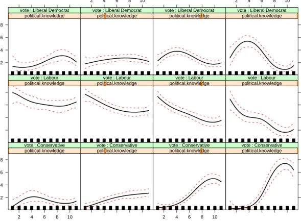
Figure 3: Effect plot for theEurope×political.knowledgeinteraction in the multinomial logit model fit to theBEPS data.
To obtain “safe predictions” of the effects in a model that uses a data-dependent basis for the model matrix (such as the present model, which employs a regression spline), theeffect function refits the model, adapting the strategy described inHastie(1992, Section 7.3.3). To produce a smooth graph, we set Europe to 50 evenly spaced values between 1 and 11, even though the variable itself takes on only integer values; political.knowledgeis set to integer values between 0 and 3; the dummy regressor for gender,gendermale, is fixed to 0.5, representing a group composed equally of men and women. The default effect plot for the Europe× political.knowledgeinteraction is shown in Figure 3:
R> plot(europe.knowledge)
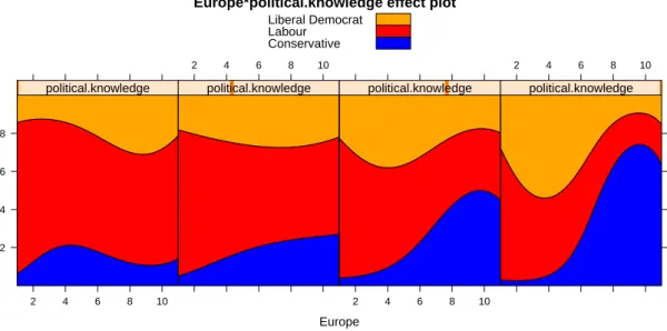
An alternative “stacked-area” representation of the interaction, using traditional political-party colors (and suppressing the uninformative rug-plot at the bottom of each panel), is displayed in Figure4:
R> plot(europe.knowledge, style = "stacked",
Europe*political.knowledge effect plot Europe vote (probability) 0.2 0.4 0.6 0.8 2 4 6 8 10 political.knowledge 2 4 6 8 10 political.knowledge 2 4 6 8 10 political.knowledge 2 4 6 8 10 political.knowledge Liberal Democrat Labour Conservative
Figure 4: Alternative “stacked-area” effect display for theEurope × political.knowledge interaction.
It is clear from both effect displays that as voters’ knowledge increased, they more accurately aligned their votes with their political opinions: At the lowest level of political knowledge (the left-most column of Figure 3 and the left panel of Figure 4), the relationship between attitude towards European integration and vote was weak, and indeed there was slightly higher support for the pro-Europe Liberal Democratic Party among the most Eurosceptic voters than among those most favorable to European integration of the UK. At the highest level of political knowledge, support for the anti-Europe Conservative Party increased dramatically with opposition to European integration, as support for Labour and the Liberal Democrats declined. The confidence envelopes in Figure 3 show that these effects are quite precisely estimated.
We reiterate that the use of a regression spline in this model makes direct interpretation of the estimated coefficients a practical impossibility. Even if the we had fit a linear term in attitude towards European integration, however, the complicated structure of the multinomial logit model together with the interaction between attitude towards Europe and political knowledge would have proved an obstacle to direct interpretation of the coefficients.
3. Effect displays for proportional-odds models
The proportional-odds model, perhaps the regression model most commonly used for an ordinal response, is often derived by assuming a linear regression for a latent response variables ξ,
ξi =α+x0iβ+εi=α+ηi+εi (2) where x0i is the ith row of the model matrix, β is a vector of regression coefficients, andα is an intercept parameter (which will prove redundant). Although the latent response cannot
be observed directly, a binned version of it,y, withm levels is available: yi = 1 for ξi≤α1 2 for α1 < ξi ≤α2 .. . m−1 for αm−2 < ξi ≤αm−1 m for αm−1 < ξi
where the “thresholds,”α1 < α2<· · ·< αm−1, are parameters to be estimated from the data
along with the regression coefficients. The cumulative distribution function of the observed response is
Pr(yi ≤j) = Pr(ξi≤αj)
= Pr(α+ηi+εi ≤αj) = Pr(εi ≤αj−α−ηi)
for j = 1,2, ..., m−1. Assuming that the errors εi are normally distributed produces an ordered probit model; assuming that the errors are logistically distributed, with distribution function
Λ(εi) = 1 1 +e−εi produces an ordered logit model:
logit[Pr(yi > j)] = loge
Pr(yi > j) Pr(yi ≤j)
=−αj+x0iβ, forj = 1,2, ..., m−1 (3) The intercept α in Equation 2 is set to 0 to identify the model, in effect fixing the origin of the latent response. This model is called the “proportional-odds model” because different cumulative log-odds, logit[Pr(yi > j)] and logit[Pr(yi > j0)], differ by the constant αj0 −αj, and therefore the odds themselves are proportional regardless of the value of x0i. Each level of y save the last has its own intercept, which is the negative of the corresponding threshold, but there is a common coefficient vector β.
The WVS data frame in theeffects package contains data from the second wave of the World Value Survey (Inglehart 2000), conducted between 1995 and 1997. Forty-two countries par-ticipated in this survey, which collected data on social attitudes and related information employing a common questionnaire. We focus here on four countries (with sample sizes given in parentheses): Australia (1874), Norway (1127), Sweden (1003), and the United States (1377). The response variable in our illustration, which is adapted from, but not identical to, an example in Fox and Andersen (2006), is the answer to the question, “Do you think that what the government is doing for people in poverty in this country is about the right amount, too much, or too little?” Predictors include country, gender, religion (whether or not the respondent belonged to a religion), education (whether or not the respondent held a university degree), and age (in years):
poverty religion degree country age Too Little :2708 no : 786 no :4238 Australia:1874 Min. :18.00 About Right:1862 yes:4595 yes:1143 Norway :1127 1st Qu.:31.00 Too Much : 811 Sweden :1003 Median :43.00 USA :1377 Mean :45.04 3rd Qu.:58.00 Max. :92.00 gender female:2725 male :2656
The commandexample(WVS)will reproduce the results in this section.
After exploring the data, we fit the following model, which includes interactions between country and the other predictors (because the focus here is on national differences), and employs a four-degree-of-freedom regression spline in age. We employ thepolrfunction in the
MASSpackage (associated withVenables and Ripley 2002), which is one of the recommended packages in R:
R> wvs.1 <- polr(poverty ~ country*(gender + religion + degree + bs(age, 4)),
+ data = WVS)
R> Anova(wvs.1)
Anova Table (Type II tests) Response: poverty LR Chisq Df Pr(>Chisq) country 243.522 3 < 2.2e-16 *** gender 11.469 1 0.0007077 *** religion 4.161 1 0.0413731 * degree 3.954 1 0.0467681 * bs(age, 4) 63.749 4 4.721e-13 *** country:gender 3.666 3 0.2998727 country:religion 21.229 3 9.437e-05 *** country:degree 13.071 3 0.0044859 ** country:bs(age, 4) 39.015 12 0.0001046 *** ---Signif. codes: 0 '***' 0.001 '**' 0.01 '*' 0.05 '.' 0.1 ' ' 1 Eliminating the nonsignificant interaction between country and gender yields
R> wvs.2 <- polr(poverty ~ gender + country*(religion + degree + bs(age, 4)),
+ data = WVS)
R> summary(wvs.2)
Re-fitting to get Hessian Call:
polr(formula = poverty ~ gender + country * (religion + degree + bs(age, 4)), data = WVS)
Coefficients:
Value Std. Error t value gendermale 0.18063079 0.05336493 3.3848223 countryNorway 0.78121663 0.37942412 2.0589535 countrySweden 0.92681750 0.61091266 1.5171031 countryUSA 0.06582379 0.39913430 0.1649164 religionyes 0.02907219 0.11255775 0.2582869 degreeyes -0.13419407 0.16864178 -0.7957345 bs(age, 4)1 0.94921130 0.39894576 2.3792991 bs(age, 4)2 1.28306334 0.37368792 3.4335157 bs(age, 4)3 1.28795735 0.56139196 2.2942212 bs(age, 4)4 1.54719724 0.55650180 2.7802197 countryNorway:religionyes -0.24538680 0.21596212 -1.1362493 countrySweden:religionyes -0.93870016 0.51184358 -1.8339590 countryUSA:religionyes 0.56612729 0.17405513 3.2525745 countryNorway:degreeyes 0.06813722 0.20910716 0.3258483 countrySweden:degreeyes 0.66297579 0.21686252 3.0571249 countryUSA:degreeyes 0.29178752 0.20773850 1.4045905 countryNorway:bs(age, 4)1 -0.46956213 0.60162430 -0.7804906 countrySweden:bs(age, 4)1 -0.34517378 0.66252453 -0.5209977 countryUSA:bs(age, 4)1 0.76323525 0.64214454 1.1885724 countryNorway:bs(age, 4)2 -1.44786885 0.66459380 -2.1785771 countrySweden:bs(age, 4)2 -1.74712063 0.76337334 -2.2886844 countryUSA:bs(age, 4)2 -1.84850957 0.59259945 -3.1193238 countryNorway:bs(age, 4)3 -1.23552288 1.08132883 -1.1425968 countrySweden:bs(age, 4)3 -0.21821661 1.28320100 -0.1700565 countryUSA:bs(age, 4)3 2.01537772 0.85772545 2.3496770 countryNorway:bs(age, 4)4 -0.21080180 1.62185112 -0.1299760 countrySweden:bs(age, 4)4 -0.82992489 2.28421574 -0.3633303 countryUSA:bs(age, 4)4 -1.35489504 0.84068831 -1.6116497 Intercepts:
Value Std. Error t value Too Little|About Right 1.1117 0.2472 4.4969 About Right|Too Much 2.9382 0.2500 11.7539 Residual Deviance: 10315.45
AIC: 10375.45
As was true of the multinomial-logit model, it is difficult to interpret the results from the estimated coefficients. We will instead present three illustrative effect displays for the country × age interaction. The first display (Figure 5), which is the default, includes point-wise confidence bands around the fitted effect:
country*age effect plot age poverty (probability) 0.2 0.4 0.6 0.8 20 40 60 80 : country Australia : poverty Too Little
: country Norway
: poverty Too Little
20 40 60 80
: country Sweden
: poverty Too Little
: country USA
: poverty Too Little :
country Australia :
poverty About Right
: country Norway
:
poverty About Right
: country Sweden
:
poverty About Right
0.2 0.4 0.6 0.8 : country USA :
poverty About Right 0.2 0.4 0.6 0.8 : country Australia : poverty Too Much
20 40 60 80
: country Norway
: poverty Too Much
: country Sweden
: poverty Too Much
20 40 60 80
: country USA
: poverty Too Much
Figure 5: Effect display for the country × age interaction in the proportional-odds logit model fit to theWVSdata.
R> with(WVS, quantile(age, c(0, .01, .99, 1)))
0% 1% 99% 100% 18 18 83 92
R> plot(effect("country*bs(age,4)", wvs.2, xlevels = list(age = 18:83),
+ given.values = c(gendermale = 0.5)), rug = FALSE)
Because there are a few very old individuals in the data set, we plot to the 99th percentile of age, setting age to integer values between 18 and 83 (which produces a smooth plot). We also fix the proportion of men to 0.5; religion and education are implicitly set to their observed proportions in the data (which are, respectively, 0.85 church attenders and 0.21 with post-secondary degrees).
The second display (Figure 6) is a “stacked-area” graph, obtained by setting the argument style="stacked"to theplotmethod for polytomous effect-display objects:
country*age effect plot age poverty (probability) 0.2 0.4 0.6 0.8 20 30 40 50 60 70 80 : country Australia 20 30 40 50 60 70 80 : country Norway 20 30 40 50 60 70 80 : country Sweden 20 30 40 50 60 70 80 : country USA Too Much About Right Too Little
Figure 6: Stacked-area effect plot for thecountry× ageinteraction.
R> plot(effect("country*bs(age,4)", wvs.2, xlevels = list(age = 18:83),
+ given.values = c(gendermale = 0.5)), rug = FALSE, style = "stacked")
The colors for the levels of the ordered response are selected using thesequential_hcl func-tion in thecolorspacepackage (Ihaka, Murrell, Hornik, and Zeileis 2009;Zeileis, Hornik, and
Murrell 2009); default colors for multinomial logit models are selected using therainbow_hcl
function in the same package.
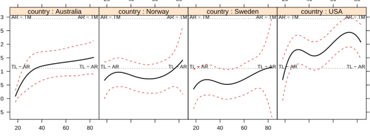
Finally, Figure7shows an effect display for the country-by-age interaction on the scale of the latent response, obtained by specifying the argumentlatent=TRUE to theeffect function:
R> plot(effect("country*bs(age,4)", wvs.2, xlevels = list(age = 18:83),
+ given.values = c(gendermale = 0.5), latent = TRUE), rug = FALSE)
Notice that the display includes horizontal lines at the category thresholds of the response. The three displays reveal a similar pattern: Support for government action for the poor generally declined with age in all four countries, but the relationship to age was stronger in Australia and the US than in Norway or Sweden, and at virtually all ages, support for the poor was lower in the US than in the other three countries. The estimated modal response in Norway and Sweden was ‘too little’ at virtually all ages, and ‘about right’ in the US at almost all ages; in Australia, the modal response was ‘too little’ among young respondents and ‘about right’ among older respondents. Figure 5 suggests that probabilities of category membership are estimated with reasonable precision, except at the highest ages in Norway and Sweden, but Figure7shows that there is substantial uncertainty in the estimated effects on the scale of the latent response.
As in the previous example, the use of a B-spline in this model, here for age, makes it impractical to interpret the coefficient estimates directly. Had we specified a linear effect for
country*age effect plot
age
poverty: Too Little, About Right, Too Much
−0.5 0 0.5 1 1.5 2 2.5 3 20 40 60 80 TL − AR AR − TM TL − AR AR − TM : country Australia 20 40 60 80 TL − AR AR − TM TL − AR AR − TM : country Norway 20 40 60 80 TL − AR AR − TM TL − AR AR − TM : country Sweden 20 40 60 80 TL − AR AR − TM TL − AR AR − TM : country USA
Figure 7: Effect display for thecountry× ageinteraction, plotted on the scale of the latent response. The horizontal lines give the estimated thresholds between levels of the observed response.
age, direct interpretation would have been possible in principle, at least on the scale of the latent response, but would have required mental arithmetic to sum coefficients marginal to each high-order term.
Acknowledgments
The work reported here was partly supported by research grants to John Fox from the Social Sciences and Humanities Research Council of Canada and McMaster University. We are also grateful to Michael Friendly for several suggestions.
References
Andersen R, Heath A, Sinnott R (2002). “Political Knowledge and Electoral Choice.”British Elections and Parties Review,12, 11–27.
Fisher RA (1936). Statistical Methods for Research Workers. 6th edition. Oliver and Boyd, Edinburgh.
Fox J (1987). “Effect Displays for Generalized Linear Models.” In CC Clogg (ed.),Sociological Methodology, volume 17, pp. 347–361. American Sociological Association, Washington DC. Fox J (2003). “Effect Displays in R for Generalised Linear Models.” Journal of Statistical
Software,8(15), 1–27. URL http://www.jstatsoft.org/v08/i15/.
Fox J (2008). Applied Regression Analysis and Generalized Linear Models. 2nd edition. Sage, Thousand Oaks CA.
Fox J, Andersen R (2006). “Effect Displays for Multinomial and Proportional-Odds Logit Models.” In RM Stolzenberg (ed.), Sociology Methodology, volume 36, pp. 225–255. Amer-ican Sociological Association, Washington DC.
Goodnight JH, Harvey WR (1978). “Least Squares Means in the Fixed-Effect General Linear Model.”Technical Report R-103,SAS Institute, Cary NC.
Harrell Jr FE (2001). Regression Modeling Strategies: With Applications to Linear Models, Logistic Regression, and Survival Analysis. Springer-Verlag, New York.
Hastie TJ (1992). “Generalized Additive Models.” In JM Chambers, TJ Hastie (eds.), Sta-tistical Models inS, pp. 249–307. Wadsworth, Pacific Grove, CA.
Ihaka R, Gentleman R (1996). “A Language for Data Analysis and Graphics.” Journal of Computational and Graphical Statistics,5, 299–314.
Ihaka R, Murrell P, Hornik K, Zeileis A (2009). colorspace: Color Space Manipulation. R
package version 1.0-1, URL http://CRAN.R-project.org/package=colorspace.
Inglehart REA (2000). “World Value Surveys and European Value Surveys, 1981–1984, 1990– 1993, and 1995–1997 [Computer File].” Technical report, Institute for Social Research (Producer), Inter-University Consortium for Political and Social Research (Distributor), Ann Arbor, MI.
RDevelopment Core Team (2009).R: A Language and Environment for Statistical Computing.
RFoundation for Statistical Computing, Vienna, Austria. ISBN 3-900051-07-0, URLhttp: //www.R-project.org/.
Searle SR, Speed FM, Milliken GA (1980). “Population Marginal Means in the Linear Model: An Alternative to Least Squares Means.”The American Statistician,34, 216–221.
Venables WN, Ripley BD (2002).Modern Applied Statistics inS. 4th edition. Springer-Verlag, New York.
Zeileis A, Hornik K, Murrell P (2009). “Escaping RGBland: Selecting Colors for Statistical Graphics.”Computational Statistics & Data Analysis,53, 3259–3270.
A. Standard errors for the displays
This appendix adaptsFox and Andersen’s (2006) results on standard errors for effect displays in polytomous logit models to the notation of the present paper, which, in turn, reflects the parametrization of the multinomial and proportional-odds logit models in themultinomand polrfunctions.
Because the fitted probabilities in the multinomial logit model are nonlinear functions of the model parameters (from Equation 1), Fox and Andersen derive approximate standard errors for effects by the delta method. Each fitted probability for an effect is computed at a particular model vector x00; differentiating the corresponding fitted probabilities µ0j with respect to the parametersβj of the model produces
∂µ0j ∂βj = exp(x00βj)h1 +Pm k=2,k6=jexp(x00βk) i x0 [1 +Pm k=2exp(x00βk)] 2 ∂µ0j ∂βj06=j =− expx00 βj0 +βj x0 [1 +Pm k=2exp(x00βk)] 2 ∂µ01 ∂βj =− exp(x00βj)x0 [1 +Pm k=2exp(x00βk)] 2
Let Vb(βb) represent the covariance matrix of the estimated coefficients βbj stacked into a column vector, b V(βb) =Vb b β2 b β3 .. . b βm = [vst], s, t= 1, . . . , r wherer=p(m−1). Then b V(bµ0j)≈ r X s=1 r X t=1 vst ∂µb0j ∂βbs ∂µb0j ∂βbt
Because 0<µb0j <1, Fox and Andersen suggest translating to individual-category logits, λ0j = log
µ0j 1−µ0j
(4)
By a second application of the delta method,
b V(bλ0j)≈ 1 b µ20j(1−µb0j)2 b V(µb0j) (5)
Confidence bounds computed on the logit scale using the standard error q
b
V(bλ0j) can then be translated back to the probability scale.
individual-category probabilitiesµ0j = Pr(Y0=j) are required:
µ01=
1
1 + exp(−α1+η0)
µ0j =
exp(η0) [exp(−αj−1)−exp(−αj)] [1 + exp(−αj−1+η0)] [1 + exp(−αj +η0)] , j = 2, . . . , m−1 µ0m= 1− m−1 X j=1 µ0j
whereη0 = x00β is the linear predictor at the focal model-vector x00. The derivatives of µ0j with respect to the parameters of the model (thresholdsαj and regression coefficients β) are
∂µ01 ∂α1 =− exp(−α1+η0) [1 + exp(−α1+η0)]2 ∂µ01 ∂αj = 0, j= 2, . . . , m−1 ∂µ01 ∂β =− exp(−α1+η0)x0 [1 + exp(−α1+η0)]2 ∂µ0j ∂αj−1 = exp(−αj−1+η0) [1 + exp(−αj−1+η0)]2 ∂µ0j ∂αj =− exp(−αj+η0) [1 + exp(−αj+η0)]2 ∂µ0j ∂αj0 = 0, j 0 6=j, j−1 ∂µ0j ∂β =
exp(η0) [exp(−αj)−exp(−αj−1)] [exp(−αj−1−αj+ 2η0)−1]x0
[1 + exp(−αj−1+η0)]2[1 + exp(−αj+η0)]2 ∂µ0m ∂αm−1 = exp(−αm−1+η0) [1 + exp(−αm−1+η0)]2 ∂µ0m ∂αj = 0, j= 1, . . . , m−2 ∂µ0m ∂β = exp(−αm−1+η0)x0 [1 + exp(−αm−1+η0)]2
Stacking all of the parameters in the vector γ= (α1, . . . , αm−1,β0)0, b V(γb) = [vst], s, t= 1, . . . , r wherer=m+p−2. Then, b V(bµ0j)≈ r X s=1 r X t=1 vst ∂µb0j ∂bγs ∂µb0j ∂γbt
Aproximate variances of the individual-category logits follow from Equations4 and 5, as in the multinomial logit model.
Affiliation: John Fox
Department of Sociology McMaster University 1280 Main Street West
Hamilton, Ontario, Canada L8S 4M4 E-mail: [email protected]
URL:http://socserv.socsci.mcmaster.ca/jfox/
Journal of Statistical Software
http://www.jstatsoft.org/ published by the American Statistical Association http://www.amstat.org/Volume 32, Issue 1 Submitted: 2009-04-17