Operator Splitting Methods for Convex and Nonconvex Optimization

UCLA

UCLA Electronic Theses and Dissertations

Operator Splitting Methods for Convex and Nonconvex Optimization Permalink https://escholarship.org/uc/item/78q0n13c Author Liu, Yanli Publication Date 2020 Peer reviewed|Thesis/dissertation

UNIVERSITY OF CALIFORNIA Los Angeles

Operator Splitting Methods for Convex and Nonconvex Optimization

A dissertation submitted in partial satisfaction of the requirements for the degree Doctor of Philosophy in Mathematics

by

Yanli Liu

c

Copyright by Yanli Liu

ABSTRACT OF THE DISSERTATION

Operator Splitting Methods for Convex and Nonconvex Optimization

by

Yanli Liu

Doctor of Philosophy in Mathematics University of California, Los Angeles, 2020

Professor Wotao Yin, Chair

This dissertation focuses on a family of optimization methods called operator split-ting methods. They solve complicated problems by decomposing the problem structure into simpler pieces and make progress on each of them separately. Over the past two decades, there has been a resurgence of interests in these methods as the demand for solving structured large-scale problems grew. One of the major challenges for split-ting methods is their sensitivity to ill-conditioning, which often makes them struggle to achieve a high order of accuracy. Furthermore, their classical analyses are restricted to the nice settings where solutions do exist, and everything is convex. Much less is known when either of these assumptions breaks down.

This work aims to address the issues above. Specifically, we propose a novel acceler-ation technique called inexact preconditioning, which exploits second-order informacceler-ation at relatively low computation cost. We also show that certain splitting methods still work on problems without solutions, in the sense that their iterates provide information on what goes wrong and how to fix. Finally, for nonconvex problems with saddle points, we show that almost surely, splitting methods will only converge to the local minimums under certain assumptions.

The dissertation of Yanli Liu is approved.

Ali H. Sayed Lieven Vandenberghe

Luminita Aura Vese Wotao Yin, Committee Chair

University of California, Los Angeles 2020

Contents

List of Figures . . . . x

List of Tables . . . . xii

Acknowledgments . . . . xiii

Curriculum Vitae . . . . xiv

I

Introduction

1

1.1 Background . . . 3

1.2 Operator Splitting Methods . . . 4

1.3 Contributions . . . 5

1.3.1 Acceleration by inexact preconditioning . . . 5

1.3.2 Convergence behavior on pathological problems . . . 7

1.3.3 Convergence behavior on nonconvex problems . . . 8

1.4 Notations and Preliminaries . . . 9

1.5 Common Operator Splitting Schemes . . . 11

II

Acceleration by Inexact Preconditioning

15

2.1.1 Proposed approach . . . 18 2.1.2 Related Literature . . . 20 2.1.3 Organization . . . 21 2.2 Preliminaries . . . 22 2.3 Main results . . . 22 2.3.1 Preconditioned PDHG . . . 23 2.3.2 Choice of preconditioners. . . 24

2.3.3 PrePDHG with fixed inner iterations . . . 26

2.3.4 Global convergence of iPrePDHG . . . 30

2.4 Numerical experiments . . . 39

2.4.1 Graph cuts . . . 43

2.4.2 Total variation based image denoising . . . 44

2.4.3 Earth mover’s distance . . . 47

2.4.4 CT reconstruction . . . 49

2.5 Conclusion . . . 50

2.A ADMM as a special case of PrePDHG . . . 52

2.B Proof of Theorem 2.3.4: bounded relative error whenS is the iterator of cyclic proximal BCD . . . 54

2.C Two-block ordering in Claim 2.4.1 and four-block ordering in Claim 2.4.2 56 3 Inexact Preconditioning for SVRG and Katyusha X. . . . 58

3.1 Introduction . . . 58

3.1.1 Related Work . . . 58

3.2 Preliminaries and Assumptions . . . 61 3.3 Proposed Algorithms . . . 63 3.4 Main Theory . . . 66 3.5 Experiments . . . 71 3.5.1 Lasso . . . 72 3.5.2 Logistic Regression . . . 74 3.5.3 Sum-of-nonconvex Example . . . 76

3.6 Conclusions and Future Work . . . 77

3.A Proof of Lemma 3.4.1 . . . 78

3.B Proof of Theorem 3.4.2 . . . 84

3.C Proof of Lemma 3.4.4 . . . 91

3.D Proof of Theorem 3.4.3 . . . 91

3.E Proof of Theorems 3.4.5 and 3.4.6 . . . 92

III

Convergence Behaviors on Pathological Problems

95

4.1 Introduction . . . 97

4.1.1 Basic definitions. . . 99

4.1.2 Classification of conic programs . . . 100

4.1.3 Classification method overview . . . 105

4.1.4 Previous work . . . 106

4.2 Obtaining certificates from Douglas-Rachford Splitting . . . 106

4.2.2 Fixed-point iterations without fixed points . . . 111

4.2.3 Feasibility and infeasibility . . . 114

4.2.4 Modifying affine constraints to achieve strong feasibility . . . 118

4.2.5 Improving direction . . . 119

4.2.6 Modifying the objective to achieve finite optimal value . . . 122

4.2.7 Other cases . . . 123

4.2.8 The algorithms . . . 125

4.2.9 Case-by-case illustration . . . 126

4.3 Numerical Experiments . . . 131

5 DRS and ADMM for Pathological Convex Problems . . . . 134

5.1 Introduction . . . 134

5.1.1 Summary of results, contribution, and organization . . . 135

5.1.2 Prior work . . . 137

5.2 Preliminaries . . . 139

5.2.1 Duality and primal subvalue . . . 140

5.2.2 Douglas–Rachford operator . . . 142

5.2.3 Fixed-point iterations without fixed points . . . 142

5.3 Theoretical results . . . 143

5.3.1 Infimal displacement vector of the DRS operator. . . 145

5.3.2 Function-value analysis . . . 148

5.3.3 Evolution of shadow iterates . . . 153

5.4 Pathological convergence: DRS . . . 155

5.4.2 Convergence results . . . 158

5.4.3 Interpretation . . . 159

5.4.4 Feasibility problems. . . 160

5.5 Pathological convergence: ADMM . . . 162

5.5.1 Classification and convergence results . . . 163

5.5.2 Interpretation . . . 164

5.5.3 Proofs . . . 164

5.6 When strong duality fails . . . 165

5.7 Conclusion . . . 168

IV

Convergence Behaviors on Nonconvex Problems

169

6.1 Introduction . . . 171

6.2 Preliminaries . . . 173

6.3 Davis-Yin Splitting and its Envelope . . . 175

6.3.1 Review of Davis-Yin Splitting . . . 175

6.3.2 Envelope of Davis-Yin Splitting . . . 177

6.4 Properties of Envelope . . . 178

6.4.1 Global Minimizers Correspondence . . . 181

6.4.2 Davis-Yin Splitting as Gradient Descent of the Envelope . . . . 183

6.4.3 Local Minimizers Correspondence . . . 187

6.4.4 Critical and Stationary Point Correspondence . . . 188

6.5 Avoidance of Strict Saddle Points . . . 191

6.6 Conclusions . . . 195

List of Figures

2.1 two-block ordering in Claim 2.4.1 . . . 41

2.2 four-block ordering in Claim 2.4.2 . . . 41

2.3 Input image . . . 44

2.4 Graph cut by iPrePDHG (Inner: BCD) . . . 44

2.5 Noisy image . . . 46

2.6 Denoising by iPrePDHG (Inner: BCD) . . . 46

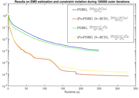
2.7 For PDHG, τ = 3×10−6_{, σ =} 1 τkdivk2; For iPrePDHG (Inner: BCD), τ = 3×10−6_{, M} 1 = τ−1In, M2 = τdivdivT, γ = _kM1_2k, and p = 2. km∗|k1,2 is obtained by calling CVX. . . 48

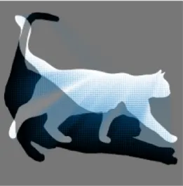
2.8 ρ0_{, ρ}1 _{are the white standing cat and the black crouching cat, respectively.} Both images are 256×256, and the earth mover’s distance between ρ0 and ρ1 _{is 0.6718. . . . . 49}

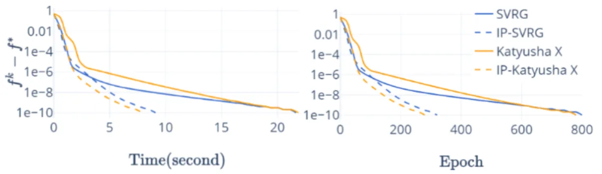
3.1 Lasso on w1a.t,(n, d) = (47272,300),λ1 = 10−3, λ2 = 10−8. For iPreSVRG and iPreKatX: η1 = 0.005; For SVRG and Katyusha X: η2 = 0.08; For Katyusha X and iPreKatX: τ = 0.45, M =M2 with α = 0.01. . . 73

3.2 Lasso on protein, (n, d) = (17766,357), λ1 = 10−4, λ2 = 10−6, η1 = 0.008, η2 = 0.2,τ = 0.2, M =M2 with α = 0.008. . . 73

3.3 Lasso on cod-rna.t, (n, d) = (271617,8), λ1 = 10−2, λ2 = 1, η1 = 1, η2 = 5×10−6_{, τ = 0.45, M =M} 1, subproblem iterator step size γ = 3×10−6. . 73

3.4 Lasso on australian, (n, d) = (690,14), λ1 = 2, λ2 = 10−8, η1 = 0.01, η2 = 8×10−10, τ = 0.49, M =M1,γ = 5×10−10. . . 74

3.5 Logistic regression onw1a.t,(n, d) = (47272,300),λ1 = 5×10−4, λ2 = 10−8, η1 = 0.06,η2 = 4, τ = 0.4, M =M2 with α= 0.005. . . 75

3.6 Logistic regression on protein, (n, d) = (17766,357), λ1 = 10−4, λ2 = 10−8,

η1 = 1.5,η2 = 10, τ = 0.3, M =M2 with α= 0.05. . . 75

3.7 Logistic regression on cod-rna.t, (n, d) = (271617,8), λ1 = 0.1, λ2 = 10−8,

η1 = 1, η2 = 3×10−5, τ = 0.4, M =M1, γ = 2×10−5. . . 76

3.8 Logistic regression on australian, (n, d) = (690,14), λ1 = 0.5, λ2 = 10−8,

η1 = 1, η2 = 10−6,τ = 0.2, M =M1, γ = 2×10−7. . . 76

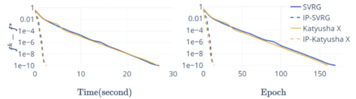
3.9 Sum-of-nonconvex on synthetic data. λ1 = 10−3, α = 15. η1 = 0.015,

η2 = 10−4, τ = 0.45. . . 77

4.1 The flowchart for identifying cases (a)–(g). A solid arrow means the cases are always identifiable, a dashed arrow means the cases sometimes identifiable.107

List of Tables

2.1 Graph cut test . . . 44

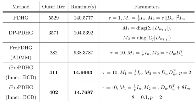
2.2 TV-L1 denoising test. PDHG is original PDHG. DP-PDHG uses diagonal preconditioning. PrePDHG uses non-diagonal preconditioning. iPrePDHG (Inner: BCD) is our algorithm that uses both non-diagonal preconditioning

and an iterator S instead of solving the z-subproblem. . . 46

2.3 CT reconstruction . . . 51

4.1 Percentage of infeasibility detection in [135], C stands for “clean" and M stands for “messy". . . 132

4.2 Percentage of infeasibility detection success, C stands for “clean" and M stands for “messy". . . 132

4.3 Percentage of success determination that problems are not strongly infeasi-ble, C stands for “clean" and M stands for “messy". . . 132

Acknowledgments

First and foremost, I would like to express my sincere gratitude to my advisor, Professor Wotao Yin, who has been a tremendous mentor during the past 5 years. Prof. Yin’s high standards in both research and presentation have greatly improved the quality of my work, and have shaped me into an independent researcher. This dissertation would not have been possible without his guidance and encouragement.

I would also like to thank my the other members of my committee, Prof. Ali H. Sayed, Prof. Lieven Vandenberghe, and Prof. Luminita A. Vese for their advice and feedback. Their knowledge and insights have greatly enriched my work.

I am also indebted to my great collaborators: Prof. Ernest Ryu for his valuable suggestions on paper writing, and for his advice on doing research in general; Fei Feng, Robert Hannah, Yuejiao Sun and Yunbei Xu for their insights and hard work on our shared projects.

My friends and colleges have affected my Ph.D. career in a very positive way, in-cluding Qi Guo, Robert Hannah, Jialin Liu, Lecheng Ruan, Tao Sun, Baichuan Yuan, and Kun Yuan. I appreciate their advice on research and life in general.

Last but not the least, I am very grateful for my family back home for their uncon-ditional love and support during this joyful journey.

Curriculum Vitae

2011 - 2015 Bachelor of Science in Physics, Minor Degree in Mathematics, Nankai University. Tianjin, China

2015 - 2020 Teaching and Research Assistant, Department of Mathematics, Uni-versity of California, Los Angeles. Los Angeles, CA, USA

2018 Research Intern, Neo IVY Capital Management, New York, USA

2019 Research Intern, Alibaba DAMO Academy, Seattle, USA

Publications

Ryu, Ernest K., Yanli Liu, and Wotao Yin. "DouglasRachford splitting and ADMM for pathological convex optimization." Computational Optimization and Applications 74.3 (2019): 747-778.

Liu, Yanli, and Wotao Yin. "An envelope for DavisYin splitting and strict saddle-point avoidance." Journal of Optimization Theory and Applications 181.2 (2019): 567-587.

Liu, Yanli, Fei Feng, and Wotao Yin. "Acceleration of SVRG and Katyusha X by Inexact Preconditioning." International Conference on Machine Learning. 2019.

Liu, Yanli, Yunbei Xu, and Wotao Yin. "Acceleration of Primal-Dual Methods by Preconditioning and Simple Subproblem Procedures." arXiv preprint arXiv:1811.08937 (2018).

Hannah, Robert, Yanli Liu, Daniel O’Connor, and Wotao Yin. "Breaking the span assumption yields fast finite-sum minimization." Advances in Neural Information

Pro-cessing Systems. 2018.

Liu, Yanli, Ernest K. Ryu, and Wotao Yin. "A new use of DouglasRachford splitting for identifying infeasible, unbounded, and pathological conic programs." Mathematical Programming 177.1-2 (2019): 225-253.

Chang, Joshua C., Yanli Liu, and Tom Chou. "Reconstruction of Cell Focal Adhesions using Physical Constraints and Compressive Regularization." Biophysical journal 113.11 (2017): 2530-2539.

Part I

CHAPTER 1

Introduction

This dissertation focuses on solving structured optimization problems. Specifically, we consider the composite optimization problem of the following form:

minimizef(x) +g(x), (1.1)

where f and g are functions with special structures and can be nonsmooth or noncon-vex. Common examples include the ℓ1−norm kxk1, the indicator function δC(x) of a

nonempty convex set C, and the finite sum f(x) = _n1Pn_i=1fi(x). Formulation (1.1)

captures problems in numerous research areas such as statistical and machine learning, medical imaging, compressed sensing, and control theory.

In these applications, the problem dimension (e.g., the size of the optimization variable x) is often very large, and the per-iteration computation cost of second-order methods (e.g., interior-point methods) is prohibitively high. Therefore, to solve (1.1)

efficiently,first-order methodsare widely applied. Among them,operator splitting meth-ods are popular choices since they can decompose complicated problem structures into smaller pieces, and lead to simple algorithms that are easy to implement and have low per-iteration cost. This dissertation aims to accelerate the convergence of operator splitting methods and to analyze their behavior in the pathological1 _{and nonconvex} settings.

1.1

Background

Since the 1980s, a family ofsecond-order methods calledinterior-point methods (IPMs) have been studied intensively by the optimization research community. In these meth-ods, the key feature is the use oflogarithmic barrier functionto incorporate the problem constraints, and the logarithmic function serves well as a barrier function due to its self-concordance property [161]. IPMs were first applied for linear programs [98]. Soon after the important role of logarithmic barrier functions was understood, IPMs were general-ized to quadratic and nonlinear problems [222]. Today, IPMs have been implemented efficiently in popular software packages [5, 166], and are often very suitable to solve problems of small or medium size. However, for many very large-scale problems that arise in modern machine learning, IPMs are often inefficient since at each iteration, IPMs require solving a linear system that involves second-order information of the ob-jective. This linear system scales as the problem dimension and leads to a prohibitive per-iteration computation cost.

In view of this, much attention in optimization research has been directed to first-order methods in the past two decades. These methods only use first-order information

such as gradient, subgradient, and proximal mapping1_{, which are often cheap to obtain,} and their cost scales well with the problem dimension. As a result, these methods are often easy to implement and enjoy low per-iteration cost. Two most prototypical examples are gradient descent and proximal point method [192], which only require evaluations of gradient or proximal mapping at each iteration. This makes them distinct from Newton’s method, which is a classical second-order method. Aside from the aforementioned advantages, first-order methods are also amenable to parallelization, which is preferable for training large-scale models. One of the most notable examples is the widely applied Stochastic Gradient Descent (SGD) [189] for neural network training.

1_{The proximal mapping for a function f is defined asProx}

f(x) = arg miny{f(y) + 12ky−xk 2_{}, a}

Based on gradient descent and proximal point method, numerous first-order algo-rithms have been developed. Some of the most popular prominent examples are, accel-erated gradient methods [163, 29], stochastic gradient methods [189,115], subgradient methods [205,181, 205], mirror descent [159,51,28], coordinate descent [182, 113, 75], conditional gradient methods [93,123,79], andoperator splitting methods that include, proximal gradient methods [133], Alternating Direction Method of Multipliers (ADMM) [94, 104], and Primal-Dual Hybrid Gradient (PDHG) [244, 49], and many other exten-sions. These methods are designed for different problem settings, but are related to each other in different ways. Furthermore, combining their features may lead to new algorithms that can solve more chanllenaging problems.

1.2

Operator Splitting Methods

Operator splitting methods are a family of first-order methods as they only rely on the first-order information of the objective. Their study originated from the seminal work by Sophus Lie on the Lie scheme in the 1890s [128]. At first, they were designed to solve the PDEs arising from computational physics. Later in the 1970s, the theory of monotone operators came into play, and these optimization methods were related to certain operator splitting schemes. For example, the projected gradient method corresponds to forward-backward splitting (FBS) [133], and the Alternating Direction Method of Multipliers (ADMM) corresponds to Douglas-Rachford splitting (DRS) [94]. This interpretation provides a unified view for these methods and has inspired the design and analysis of new optimization methods [69,62,235, 218,45]. An overview of several common splitting methods can be found in Section1.5.

The underlying principle of splitting methods is to decompose complicated problem structures into simple components, and deal with them separately by solving subprob-lems that only involve individual components. Another feature is that some of these components are allowed to be nonsmooth. In the past 15 years or so, optimization

mod-els in numerous research areas require solving nonsmooth optimization problems that are built up from simple components. To name a few, compressed sensing [76], Lasso [217], logistic regression [117] and image denoising [151] all involve sums of multiple functions and require an ℓ1−norm penalty term to promote sparsity in their solutions.

Therefore, the aforementioned advantages have led to the recent resurgence of interest in operator splitting methods.

However, splitting methods often suffer from their sensitivity to ill-conditioning, which is a common challenge for other first-order methods as well, due to the lack of second-order information. Furthermore, The classical analyses of splitting methods are constrained to non-pathological settings, where a primal-dual solution pair is assumed to exist, and strong duality holds. While in fact, even simple convex problems may not satisfy these assumptions1_{. Finally, the classical theory of splitting methods heavily} relies on the monotonicity of the individual operators, which is lacking under nonconvex settings.

This dissertation aims to accelerate the convergence of operator splitting algorithms for convex problems and to analyze their behaviors in the pathological and nonconvex settings. The contributions are listed as follows.

1.3

Contributions

1.3.1 Acceleration by inexact preconditioning

As first-order algorithms, operator splitting methods suffer from slow (tail) convergence, especially on poorly conditioned problems. They may take thousands of iterations and still struggle to reach four digits of accuracy. While they have many advantages such as being easy to implement and friendly to parallelization, their sensitivity to problem conditions is their main disadvantage.

1_{For example, consider the following two problems: (i)min}

To improve their performance of on ill-conditioned problems, researchers have tried to apply preconditioning, which is an idea first proposed for solving linear systems, and later applied to simple algorithms such as gradient descent. Recently, it has also been widely applied on splitting methods such as forward-backward splitting (FBS) [224,

61, 45, 230], Douglas-Rachford splitting (DRS) [42, 43], Primal-Dual Hybrid Gradient (PDHG) [179], and alternating directions method of multipliers (ADMM).[99, 100].

Depending on the application and how one applies splitting, these preconditioned algorithms may or may not have subproblems with closed-form solutions. When they do not, the cost of solving subproblems has to be taken into consideration. Previous works either assume the existence of an oracle that returns the exact solution of the subproblems, or allow approximate subproblem solutions with quickly diminishing er-rors [185,83, 164,126, 87, 86]. In either of these two cases, the total cost is prohibitive under realistic settings.

In Part IIof this dissertation, we present a new preconditioning technique called in-exact preconditioning and apply it to PDHG, ADMM, and Stochastic Variance-Reduced Gradient (SVRG). Conceptually, this technique involves two steps. First, one selects ap-propriate preconditioners based on specific problem structures and splitting algorithms. Then, one applies the preconditioned algorithms and solve the subproblemshighly inex-actly bywarmstart and a fixed number of simple subroutines. Efficient subroutines can be chosen based on different subproblem structure and in particular, one does not need to enforce the errors to be diminishing in certain ways as in previous works. Theoreti-cally, We show that this inexact preconditioning strategy brings significant acceleration to PDHG, ADMM, and SVRG. In practice, the efficacy of inexact preconditioning is demonstrated on several popular models such as logistic regression, graph cut, and computed tomography (CT) reconstruction, where a 4–95×speedup is observed.

1.3.2 Convergence behavior on pathological problems

Many convex optimization algorithms have strong theoretical guarantees and empirical performance, but they are often limited to non-pathological problems1; under patholo-gies often the theory breaks down and the empirical performance degrades significantly. In fact, the behavior of convex optimization algorithms under pathologies has been studied much less, and many existing solvers often simply report “failure” without in-forming the users of what went wrong upon encountering infeasibility, unboundedness, or other pathologies. Pathological problems are numerically challenging, but they are not impossible to deal with. As pathologies can arise in practice (see, for example, [141, 140, 225, 229, 78]), designing a robust algorithm that behaves well in all cases is important to the completion of a robust solver.

In Part III of this dissertation, we study the behavior of DRS and ADMM for pathological convex programs. Perhaps surprisingly, we show that although the iterates of DRS and ADMM diverge for pathological problems, the precise manner in which they diverge still provides useful information regarding the type of pathology that we encounter. Specifically, for a class of convex programs calledconic programming, many pathologies can be identified by investigating the divergence pattern of the iterates. Furthermore, for certain types of pathologies, this divergence pattern informs us how to modify the pathological program to remove the pathology. For general convex problems, certain pathologies can still be identified, and we establish that DRS and ADMM only require strong duality to work even when the primal and/or dual solution does not exist, in the sense that the objective values of the iterates are asymptotically optimal.

1.3.3 Convergence behavior on nonconvex problems

Operator splitting methods are traditionally analyzed under the assumption that the subdifferentials of the objective functions are maximally monotone. While for non-convex functions, their subdifferentials are generally non-monotone. Therefore, the majority of the existing results on splitting methods apply only to convex objective functions. Recently, FBS and DRS are found to numerically converge for certain non-convex problems [209,215,125,6,54]. Theoretically, their iterates have been shown to converge to stationary points under some nonconvex settings [10, 125, 216, 108]. How-ever, it remains possible that the limits of their convergent sequences are saddle points instead of local minimums.

In Part IV of this dissertation, we show that under some smoothness conditions, FBS and DRS can avoid the strict saddle points1 almost surely, in the sense that the probability for DRS and FBS iterations with random initializations to converge to strict saddle points of their respective objectives is zero. The main technical tools to achieve this are (i) Forward-Backward Envelope (FBE) [215], Douglas-Rachford Enve-lope (DRE) [171] from nonconvex analysis, and (ii) Stable-Center Manifold Theorem [206] from dynamical systems.

FBE and DRE are functions with nice properties even in the nonconvex settings. In particular, they share the same stationary points, local minimizers, and strict saddle points with the objectives of FBS and DRS, respectively. Furthermore, the FBS and DRS iterations can be written as (preconditioned) gradient descent iterations on FBE and DRE. By analyzing these gradient descent iterations with the Stable-Center Man-ifold Theorem, one can show that whenever FBS and DRS converge, their limits will not be the strict saddles of FBE and DRE almost surely, which are exactly the strict saddles of their corresponding objective functions. Consequently, for many practical models that satisfy thestrict saddle property2_{, FBS and DRS will almost always avoid}

the strict saddle points whenever they converge.

1.4

Notations and Preliminaries

In this section, we review standard notions of convex analysis, state several known results, and set up the notation. For the sake of brevity, we omit proofs or direct references of the standard results and refer interested readers to standard references such as [190, 195, 17]. Other relevant results will be provided at the beginning of each chapter.

We use k · k for ℓ2−norm, k · k1 for ℓ1−norm, and h·,·i for dot product. We useIn

to denote the identity matrix of size n×n. M 0 means M is a symmetric, positive definite matrix, andM 0means M is a symmetric, positive semidefinite matrix.

We write λmin(M) and λmax(M) as the smallest and the largest eigenvalues of M, respectively, andκ(M) = λmax(M)

λmin(M) as the condition number of M. ForM 0, letk · kM

and h·,·iM denote the semi-norm and inner product induced by M, respectively, i.e.,

hx, yiM =xTM y,kxkM =

√

xT_{M x. If M 0, then} k · k

M is a norm.

A function f is convex iff(θx+ (1−θ)y)≤θf(x) + (1−θ)f(y)for all x, y ∈Rnand

θ∈[0,1]. A functionf is closed if its epigraphn(x, α)∈Rn+1 _{| f(x)≤α}o _{is a closed}

subset of Rn+1. We say f :Rn →R∪ {∞} is proper if f(x)< ∞ for some x. In this work, we focus our attention on proper, closed, and convex (PCC) functions most of the time. Iffandgare PCC functions, thenf+gis PCC orf+g =∞everywhere. Ifγ >0, then γf is PCC. Define the (effective) domain of f as domf ={x ∈Rn|_{f(x) <}∞}_.

For anyγ >0, we have domγf =domf.

For a proper closed convex function f : Rn → R∪ {₊∞}_{, its subdifferential at}

x∈domf is written as

∂f(x) = {v ∈Rn |f(z)≥f(x) +hv, z−xi, ∀z ∈Rn},

and its convex conjugate as

f∗(y) = sup

x∈Rn{hy, xi −f(x)}.

We havey ∈∂f(x) if and only if x∈∂f∗(y).

If f is convex and proper, then f∗ : Rn → R∪ {∞} _{is PCC. If f is PCC, then}

(f∗)∗ =f. For any γ >0, we have(γf)∗(x) = γf∗(x/γ)and dom(γf)∗ =γdomf∗. If

h(x) = g(−x), thenh∗(y) =g∗(−y). We say that f :Rn _{→R is L}

f−smooth, if it is differentiable and satisfies

f(y)≤f(x) +h∇f(x), y−xi+ Lf

2 ky−xk

2_{,∀x, y ∈R}n_.

Note that a smooth functionf may be nonconvex.

We say that f is σf−strongly convex, if

f(y)≥f(x) +h∇f(x), y−xi+ σf

2 ky−xk

2_{,∀x, y ∈R}n_.

A set C is convex, if x, y ∈C and θ ∈[0,1]implies θx+ (1−θ)y∈C. WriteC for the closure ofC. If C is convex C is convex. The Minkowski sum and differences of A

and B are

A+B ={a+b|a∈A, b ∈B}, A−B ={a−b|a∈A, b ∈B},

respectively. If A and B are convex, then A+B and A −B are convex. However, neitherA+B nor A−B is guaranteed to be closed, even when Aand B are nonempty closed convex sets.

For the distance between x∈Rn and the set A, write

dist(x, A) = inf{kx−ak |a ∈A}.

For the distance between A and B, write

Note thatdist(A, B) = 0 if and only if0 ∈A−B.

Define the projection onto C as ΠC(x0) = arg minx∈Ckx−x0k. When C is closed

and convex,ΠC :Rn→Rn is well-defined, i.e., the minimizer uniquely exists.

Define the indicator function with respect to C as

δC(x) =      0 if x∈C, ∞ otherwise. When C is closed convex,δC :Rn→R∪ {∞} is PCC.

Define the support function of C as

σC(y) = sup x∈C{h

x, yi}.

σC : Rn → R∪ {∞} is PCC. When C is convex, we have σC = σ_C. If A and B are

convex, thenσA+B =σA+σB. If C is closed and convex, then (σC)∗ =δC.

Define the proximal operator Proxf :Rn→Rn as

Proxf(z) = arg min x∈Rn

n

f(x) + (1/2)kx−zk2o.

Whenf is PCC, thearg minuniquely exists, and thereforeProxf is well-defined. When

C is closed and convex, ProxδC = ΠC. When f is PCC, Proxf+ Proxf∗ = I, where

I :Rn→Rn is the identity operator.

A mappingT :Rn _→Rn_{is nonexpansive ifkT(x)−T(y)k ≤ kx−ykfor allx, y ∈R}n_.

Nonexpansive mappings are, by definition, Lipschitz continuous with Lipschitz constant

1. T :Rn→Rn _{is firmly-nonexpansive if}

kT(x)−T(y)k2 ≤ hx−y, T(x)−T(y)i

for all x, y ∈Rn_{. Proximal and projection operators are firmly-nonexpansive.}

1.5

Common Operator Splitting Schemes

Now let us list some common operator splitting schemes. All of them can be cast as

and zk _{belongs to some Hilbert space} H_.

Forward-backward splitting (FBS)[133] FBS solves the following problem:

minimize

x∈H f(x) +g(x),

where f is PCC and smooth, and g is PCC.

Define T = Proxγg(I−γ∇f). Then, the iteration of FBS can written as

xk+1 =T xk = Proxγg xk−γ∇f(xk). Or equivalently, yk=xk−γ∇f(xk), xk+1 = Proxγg(yk), where γ >0 is a stepsize.

From the above iteration, we can see that FBS "splits" the problem by dealing with

f and g separately.

Later, we will also work on another algorithm calledStochastic Variance-Reduced Gradient (SVRG)[114], which extends FBS to the following setting:

minimize x∈H f(x) +g(x) = n X i=1 fi(x) +g(x).

Here, f admits a finite sum structure, and its full gradient∇f(xk_{)may be expensive}

to obtain when n is large. In SVRG, a cheaper semi-stochastic gradient ∇˜k _{at x}k _is

applied instead. Specifically,

˜

∇k _=∇f(xk0_{) +∇f}

ik(xk)− ∇fik(xk

0

),

where ∇f(xk0) is a previous full gradient at some iteration, and it will be recycled for some later iterations k≥k0. ik is picked uniformly at random from {1,2, ..., n}.

SVRG iteration can be then written as

xk+1 = Proxγg

xk−γ∇˜k.

Douglas-Rachford Splitting (DRS) [77] DRS solves the following problem

minimize

x∈H f(x) +g(x),

where f and g are PCC.

DefineT = 1₂I+1₂(2 Proxγg−I)(2 Proxγf −I), whereγ >0is a stepsize. Then, DRS

iteration can be written as

zk+1=T zk,

or equivalently,

xk+1/2 = Proxγf(zk),

xk+1 = Proxγg(2xk+1/2−zk),

zk+1 =zk+xk+1−xk+1/2.

We will also work on another closely related algorithm called Alternating Direc-tion Method of Multipliers (ADMM)[94,104], which solves the following problem

minimize

x∈Rp_,y∈Rq f(x) +g(y)

subject to Ax+By =c,

where f : Rp → R∪ {∞} and g : Rq → R∪ {∞} are PCC, A ∈Rn×p, B ∈ Rn×q, and

c∈Rn_, xk+1 ∈arg min x∈Rp ( f(x) +hνk, Ax+Byk−ci+ 1 2γkAx+By k₋ ck2 ) yk+1 ∈arg min y∈Rq ( g(y) +hνk, Axk+1+By−ci+ 1 2γkAx k+1_+By−ck2 ) νk+1 =νk+ (1/γ)(Axk+1+Byk+1−c).

Under mild regularity assumptions, it can be shown that DRS and ADMM are equivalent [82, 84,236].

Primal-Dual Hybrid Gradient (PDHG)[49] The method of Primal-Dual Hybrid Gradient or PDHG for solving solves

minimize

x∈Rn f(x) +g(Ax),

where f : Rn _{→ R∪{∞}, g : R}m _{→ R∪{∞} are PCC, and A ∈ R}m×n_{. PDHG refers}

to the iteration

xk+1 = Proxτ f(xk−τ ATzk),

zk+1 = Proxσg∗(zk+σA(2xk+1−xk)),

where τ, σ >0 are stepsizes.

Define A =   ∂f A T −A ∂g∗   , and let M =    1 τIn −A T −A 1_σIm   0.

Then, the above PDHG iteration can be written as

yk+1 =T yk= (I+M−1A)−1yk,

where yk _{= (x}k_{, z}k₎T_.

The operator T = (I +M−1A)−1 is firmly nonexpansive in k · kM, and yk will

Part II

Acceleration by Inexact

Preconditioning

In this part, we present theinexact preconditioningtechnique for accelerating several operator splitting algorithms, the results can also be found in [138] and [136].

The inexact preconditioning technique consists of two steps: (i) find appropriate preconditioner(s) based on the objective and the specific splitting algorithm, and (ii) solve the subproblems inexactly by just afixed number of simple subroutines.

In Chapter2, we apply this technique to accelerate PDHG and ADMM, the resulting algorithm is called inexact preconditioned PDHG (iPrePDHG), which is summarized in Algorithm2.1. First, we provide a criterion for choosing preconditioners in Lemma2.3.1

and Theorem2.3.2. It turns out that most of the time, the optimal preconditioners will be non-diagonal, and the subproblems will not have closed-form solutions. Therefore, we propose to solve them until a certain condition is satisfied (see Definition 2.3.1). Remarkably, this condition is easily satisfied by applying some simple subroutines a fixed number of times (see Theorems 2.3.3 and 2.3.4). Finally, we prove the global convergence of iPrePDHG in Theorem 2.3.9, and provide extensive numerical tests in Section2.4.

The structure of Chapter 3is similar. We aim to accelerate SVRG and Katyusha X1 by inexact preconditioning, and the new algorithms are called iPreSVRG and iPreKatX, respectively (see Algorithms 3.1 and 3.2). The preconditioner M should decrease the condition number and can vary for different objectives(see Definition3.2.3). in Section

3.5. To prove acceleration, we first show that it is fine to solve the subproblems by applying FISTA with restart a small number of times so that a certain error condition will be satisfied (see Lemmas 3.4.1 and 3.4.4). Furthermore, when this error condition is satisfied, the global convergence of iPreSVRG and iPreKatX is guaranteed (see The-orems 3.4.2 and 3.4.3). Finally, we proved the acceleration of iPreSVRG over SVRG, as well as the acceleration of iPreKatX over Katyusha X in Theorems 3.4.5 and 3.4.6. This acceleration is also observed numerically on Lasso and logistic regression.

CHAPTER 2

Inexact Preconditioning for PDHG and ADMM

2.1

Introduction

In this chapter, we consider the following optimization problem:

minimize

x∈Rn f(x) +g(Ax), (2.1)

together with its dual problem:

minimize

z∈Rm f

∗_(−AT_{z) +g}∗_{(z), (2.2)}

where f : Rn _{→ R∪{+∞} and g : R}m _{→ R∪{+∞} are closed proper convex, and}

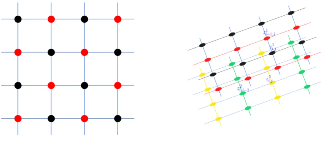
A∈Rm×n is a matrix, f∗ and g∗ are the convex conjugates off and g, respectively. Formulations (2.1) or (2.2) are abstractions of many application problems, which include image restoration [244], magnetic resonance imaging [221], network optimiza-tion [90], computer vision [180], and earth mover’s distance [127]. For many of them, primal-dual algorithms such as Primal-Dual Hybrid Gradient (PDHG) and Alternating Direction Method of Multipliers (ADMM) have been popular choices.

However, as a first-order algorithm, PDHG and ADMM suffer from slow (tail) con-vergence especially on poorly conditioned problems. They may take thousands of iter-ations and still struggle reaching just four digits of accuracy. While they have many advantages such as being easy to implement and friendly to parallelization, their sensi-tivity to problem conditions is their main disadvantage.

To improve the performance of PDHG and ADMM, researchers have tried using preconditioners, which has been widely applied for forward-backward type of methods

[224,61,45], as well as other methods [44,62, 112,223]. Depending on the application and how one applies splitting, preconditioned PDHG and ADMM may or may not have subproblems with closed-form solutions. When they do not, researchers have studied approximate subproblem solutions to reduce the total running time. In this work, we propose a new way of applying preconditioning that outperforms the existing state-of-the-art.

2.1.1 Proposed approach

Simply speaking, we find a way to have both non-diagonal preconditioners (thus much fewer iterations) and very simple subproblem procedures (thus maintaining the advan-tages of PDHG and ADMM).

First, we apply preconditioning. We present Preconditioned PDHG (PrePDHG) along with its convergence condition and a performance bound. We propose to choose preconditioners to optimize the bound. In the special case where one preconditioner is trivially fixed as an identity matrix, optimizing the bound gives us the optimal choice of the other preconditioner, which actually reduces PrePDHG to ADMM. This observation explains why ADMM often takes fewer iterations than PDHG (as PDHG sets both preconditioners to identity matrices).

Next, we study how to solve PrePDHG subproblems. In all applications we are aware of, only one of the two subproblem is (subject to) ill-conditioned. (After all, we can always apply splitting to gether ill-conditioned components into one subproblem.) Therefore, we choose a non-diagonal preconditioner for the ill-conditioned subproblem and a trivial or diagonal preconditioner for the other subproblem. Again, the pair of preconditioners should be chosen to (nearly) optimize the performance bound. Since the non-diagonal preconditioner introduces dependence between different coordinates, its subproblem generally does not have a closed-form solution. In particular, if the subproblem has anℓ1-norm, which is often the reason why PDHG or ADMM is used, it

often loses its closed-form solution due to the preconditioner. Therefore, we propose to approximately solve it to satisfy an accuracy condition. Remarkably, there is no need to dynamically stops a subproblem procedure to honor the condition. Instead, the con-dition is automatically satisfied as long as one applies a common iterative procedure for somefixed number of iterations, which is new in the literature. Common choices of the procedure include proximal gradient descent, FISTA with restart, proximal block co-ordinate descent, and accelerated block-coco-ordinate-gradient-descent (BCGD) methods (e.g., [132,3, 109]). We call this method iPrePDHG (i for “inexact”).

Next, we establish the overall convergence of iPrePDHG. To handle the inexact subproblem, we first transform iPrePDHG into an equivalent form and then analyze an Lyapunov function to establish convergence. The technique in our proof appears to be new in the PDHG and ADMM literature.

Finally, we apply our approach on a few applications including image denoising, graph cut, optimal transport, and CT reconstruction. For the last application, we use a diagonal preconditioner in one subproblem, which gives it a closed-form solution, and a non-diagonal preconditioner in the other, which we approximately solve. In each of the other applications, one subproblem uses no (identity) preconditioner, and the other uses a non-diagonal preconditioner. We numerically evaluated the performance of iPrePDHG using these recommended preconditioners and observed speedups of 4–95 times over the existing state-of-the-art.

Since we show ADMM is a special PrePDHG with one trivial preconditioner, our approach can also accelerate ADMM. In fact, for three of the above four applications, there are one trivial preconditioner in each, so their iPrePDHG are inexact precondi-tioned ADMM.

2.1.2 Related Literature

Many problems to which we apply PDHG have separable functionsf org, or both, so the resulting PDHG subproblems often (though not always) have closed-form solutions. When subproblems are simple, we care mainly about the convergence rate of PDHG, which depends on the problem conditioning. To accelerate PDHG, diagonal precondi-tioning [179] was proposed since its diagonal structure maintains closed-form solutions for the subproblems and, therefore, reduces iteration complexity without making each iteration more difficult. In comparison, non-diagonal preconditioners are much more effective at reducing iteration complexity, but their off-diagonal entries couple different components in the subproblems, causing the lost of closed-form solutions of subprob-lems.

When a PDHG subproblem has no closed-form solution, one often uses an itera-tive algorithm to approximately solve it. We call it Inexact PDHG. Under certain conditions, Inexact PDHG still converges to the exact solution. Specifically, [185] uses three different types of conditions to skillfully control the errors of the subproblems; all those errors need to be summable over all the iterations and thereby requiring the error to diminish asymptotically. In an interesting method from [42, 43], one subprob-lem computes a proximal operator of a convex quadratic function, which can include a preconditioner and still has a closed-form solution involving matrix inversion. This proximal operator is successively appliedn times in each iteration, for n ≥1.

ADMM has different subproblems. One of its subproblems minimizes the sum of

f(x)and a squared term involvingAx. Only whenAhas special structures does the sub-problem have closed-form solutions. Inexact ADMM refers to the ADMM with at least one of its subproblems inexactly solved. An absolute error criterion was introduced in [83], where the subproblem errors are controlled by a summable (thus diminishing) sequence of error tolerances. To simplify the choice of the sequences, a relative error criterion was adopted in several later works, where the subproblem errors are controlled

by a single parameter multiplying certain quantities that one can compute during the iterations. In [164], the parameters need to be square summable. In [126], the parame-ters are constants when both objective functions are Lipschitz differentiable. In [87,86], two possible outcomes of the algorithm are described: (i) infinite outer loops and finite inner loops, and (ii) finite outer loops and the last inner loop is infinite, both guarantee-ing convergence to a solution. On the other hand, it is unclear how to recognize them. Since there is no bound on the number of inner loops in case (i), one may recognize it as case (ii) and stop the algorithm before it converges.

There are works that apply certain kinds of preconditioning to accelerate ADMM. Paper [99] uses diagonal preconditioning and observes improved performance. After that, non-diagonal preconditioning is analyzed [42,43], which presents effective precon-ditioners for specific applications. One of their preconprecon-ditioners needs to be inverted (though not needed in our method). Recently, preconditioning for problems with linear

convergence has also been studied with promising numerical performances [100].

2.1.3 Organization

The rest of this chapter is organized as follows: Section 2.2 establishes notation and reviews basics. In the first part of Section 2.3, we provide a criterion for choosing preconditioners. In its second part, we introduce the condition for inexact subproblems, which can be automatically satisfied by iterating a fixed number of certain inner loops. This method is called iPrePDHG. In the last part of Section 2.3, we establish the convergence of iPrePDHG. Section 2.4 describes specific preconditioners and reports numerical results. Finally, Section2.5 concludes this chapter.

2.2

Preliminaries

In addition to the preliminaries introduced in Sec. 1.4, we need the following in this chapter.

For any M 0, we define the extended proximal operator of ϕ as

ProxM_ϕ (x) := arg min

y∈Rn {

ϕ(y) + 1

2ky−xk

2

M}. (2.3)

IfM =γ−1I forγ >0, it reduces to a classic proximal operator.

We also have the following generalization of Moreau’s Identity:

Lemma 2.2.1 ([60], Theorem 3.1(ii)). For any proper closed convex function ϕ and

M 0, we have

x= ProxM_ϕ (x) +M−1ProxM_ϕ∗−1(M x). (2.4)

We say a proper closed functionϕis a Kurdyka-ojasiewicz (KL) function if, for each

x0 ∈domϕ, there exist η∈(0,∞], a neighborhood U of x0,and a continuous concave

functionφ: [0, η)→R+ such that:

1. φ(0) = 0,

2. φ isC1 _{on (0, η),}

3. for all s∈(0, η), φ0(s)>0,

4. for all x∈U∩ {x|ϕ(x0)< ϕ(x)< ϕ(x0) +η}, the KL inequality holds:

φ0(ϕ(x)−ϕ(x0))dist(0, ∂ϕ(x))≥1.

2.3

Main results

This section presents the key results of this chapter. In Sec. 2.3.1we demonstrate how to apply preconditioning to PDHG. Then, we establish rules of preconditioner selection

in Sec. 2.3.2. In Sec. 2.3.3, we present the proposed method iPrePDHG. Finally, we establish the convergence of iPrePDHG in Sec. 2.3.4.

Throughout this section, we assume the following regularity assumptions: Assumption 2.3.1.

1. f :Rn →R∪ {₊∞}_{, g :}Rm →R∪ {₊∞} _{are proper closed convex.}

2. A primal-dual solution pair (x⋆_{, z}⋆_{) of (2.1) and (2.2) exists, i.e.,}

0∈∂f(x⋆) +ATz⋆, 0 ∈∂g(Ax⋆)−z⋆.

The problem (2.1) also has the following convex-concave saddle-point formulation:

min

x∈Rnmax_z∈Rmφ(x, z) :=f(x) +hAx, zi −g

∗_{(z). (2.5)}

A primal-dual solution pair (x⋆, z⋆) is a solution of (2.5).

2.3.1 Preconditioned PDHG

The method of Primal-Dual Hybrid Gradient or PDHG [244,49] for solving (2.1) refers to the iteration

xk+1 = Proxτ f(xk−τ ATzk),

zk+1 = Proxσg∗(zk+σA(2xk+1−xk)).

(2.6)

When _{τ σ}1 ≥ kAk2, the iterates of (2.6) converge [49] to a primal-dual solution pair of (2.1). We can generalize (2.6) by applying preconditionersM1, M2 0(their choices

are discussed below) to obtain Preconditioned PDHG or PrePDHG:

xk+1 = ProxM1 f (x k_−M−1 1 A T_zk_), zk+1 = ProxM2 g∗ (zk+M2−1A(2xk+1−xk)), (2.7)

where the extended proximal operators ProxM1

f and Prox M2

g∗ are defined in (2.3). We

There is no need to compute M₁−1 and M₂−1 since (2.7) is equivalent to xk+1 = arg min x∈Rn { f(x) +hx−xk, ATzki+1 2kx−x k_k2 M1}, zk+1 = arg min z∈Rm { g∗(z)− hz−zk, A(2xk+1−xk)i+1 2kz−z k_k2 M2}. (2.8) 2.3.2 Choice of preconditioners

In this section, we discuss how to select appropriate preconditioners M1 and M2. As

a by-product, we show that ADMM corresponds to choosing M1 = 1_τIn and optimally

choosing M2 = τ AAT, thereby, explaining why ADMM appears to be faster than

PDHG.

Let us start with the following lemma, which characterizes primal-dual solution pairs of (2.1) and (2.2).

Lemma 2.3.1. Under Assumption 2.3.1, (X, Z)is a primal-dual solution pair of (2.1)

if and only if φ(X, z)−φ(x, Z) ≤ 0 for any (x, z) ∈ Rn+m_{, where φ is given in the}

saddle-point formulation (2.5).

Proof. If(X, Z) is a primal-dual solution pair of (2.1), then −ATZ ∈∂f(X), AX ∈∂g∗(Z).

Hence, for any (x, z)∈Rn+m _{we have}

f(x)≥f(X) +h−ATZ, x−Xi, g∗(z)≥g∗(Z) +hAX, z−Zi.

Adding them together yields φ(X, z)−φ(x, Z)≤0.

On the other hand, if φ(X, z)−φ(x, Z)≤0for any (x, z)∈Rn+m_{, then}

hAX, zi+f(X)−g∗(z)− hAx, Zi −f(x) +g∗(Z)≤0 for any (x, z)∈Rn+m.

Taking x = X yields hAX, z −Zi −g∗(z) +g∗(Z) ≤ 0, so AX ∈ ∂g∗(Z); Similarly, taking z =Z gives hAX−Ax, Zi+f(X)−f(x)≤0, so −ATZ ∈∂f(X). As a result,

We present the following convergence result, adapted from Theorem 1 of [50].

Theorem 2.3.2.Let(xk, zk), k = 0,1, ..., N be a sequence generated by PrePDHG (2.7). Under Assumption 2.3.1, if in addition

˜ M :=   M1 −A T −A M2   0, (2.9)

then, for any x∈Rn _{and z} ∈Rm_{, it holds that}

φ(XN, z)−φ(x, ZN)≤ 1 2N(x−x 0_{, z−z}0₎   M1 −A T −A M2      x−x 0 z−z0   , (2.10) where XN = _N1 PN_i=1xi and ZN = _N1 PN_i=1zi.

Proof. This follows from Theorem 1 of [50] by settingLf = 0, 1_τDx(x, x0) = 1₂kx−x0k2M1,

1

σDz(z, z0) =

1

2kz −z 0_k2

M2, and K = A. Note that in Remark 1 of [50], Dx and Dz need to be1−strongly convex to ensure their inequality (13) holds, which is exactly our (2.9). Therefore, we do not need Dx and Dz to be strongly convex.

Based on the above results, one approach to accelerate convergence is to choose preconditioners M1 and M2 to obey (2.9) and minimize the right-hand side of (2.10).

When a pair of preconditioner matrices attains this minimum, we say they are optimal. When one of them is fixed, the other that attains the minimum is also called optimal.

By Schur complement, the condition (2.9) is equivalent to M2 AM1−1AT. Hence,

for any givenM1 0, the optimal M2 is AM1−1AT.

Original PDHG (2.6) corresponds to M1 = 1_τIn, M2 = 1_σIm with τ and σ obeying

1

τ σ ≥ kAk

2 _{for convergence. In Appendix 2.A, we show that ADMM for problem}

(2.1) corresponds to setting M1 = 1_τIn, M2 = τ AAT, M2 is optimal since AM1−1AT =

τ AAT = M2 (This is related to, but different from, the result in [49, Sec. 4.3] stating

that PDHG is equivalent to a preconditioned ADMM). In the next section, we show that when the z−subproblem is solved inexactly, a choice of M1 = 1_τIn, M2 =τ AAT +θIm

By using more general pairs ofM1, M2, we can potentially have even fewer iterations

of PrePDHG than ADMM.

2.3.3 PrePDHG with fixed inner iterations

It wastes total time to solve the subproblems in (2.8) very accurately. It is more efficient to develop a proper condition and stop the subproblem procedure, which we call inner iterations, once the condition is satisfied. It is even better if we can simply fix the

number of inner iterations and still guarantee global convergence.

In this subsection, we describe the “bounded relative error” of the z-subproblem in (2.7) and then show that this can be satisfied by running a fixed number of inner iterations, uniformly for every outer loop, which is new in the literature.

Definition 2.3.1 (Bounded relative error condition). Given xk_{, x}k+1 _{and z}k_{, we say}

that the z-subproblem in PrePDHG (2.7) is solved to a bounded relative error by some iterator S, if there is a constant c >0 such that

0∈∂g∗(zk+1) +M2

zk+1−zk−M₂−1A(2xk+1−xk)+εk+1, (2.11)

kεk+1k ≤ckzk+1−zkk. (2.12)

Remarkably, this condition does not need to be checked at run time. For a fixed

c > 0, the condition can be satisfied by a fixed number of inner iterations using, for example, S being the proximal gradient iteration (Theorem 2.3.3). One can also use faster solvers, e.g., FISTA with restart [167], and solvers that suit the subproblem structure, e.g., cyclic proximal BCD (Theorem 2.3.4). Although the error in solving

z-subproblems appears to be neither summable nor square summable, convergence can still be established. But first, we summarize this method in Algorithm2.1.

Theorem 2.3.3. Take Assumption2.3.1. Suppose in iPrePDHG, or Algorithm2.1, we choose S as the proximal-gradient step with stepsize γ ∈ (0,2λmin(M2)

λ2

Algorithm 2.1 Inexact Preconditioned PDHG or iPrePDHG

Input: f, g, Ain (2.1), preconditioners M1 and M2, initial (x0, z0), z-subproblem

iter-ator S, inner iteration number p, max outer iteration number K. Output: (xK_{, z}K₎ 1: for k←0,1, ..., K−1 do 2: xk+1 = ProxM1 f (xk−M− 1 1 ATzk); 3: z₀k+1 =zk_; 4: for i←0,1, ..., p−1 do 5: z_ik₊₁+1 =S(z_ik+1, xk+1_{, x}k_); 6: end for

7: zk+1 =z_pk+1; ▷which approximates ProxM2

g∗ (zk+M2−1A(2xk+1−xk))

8: end for

times, where p≥1. Then, zk+1 _=zk+1

p is an approximate solution to the z-subproblem

up to a bounded relative error in Definition 2.3.1 for

c=c(p) = 1 γ +λmax(M2) 1−ρp (ρ p +ρp−1), (2.13)

where ρ=q1−γ(2λmin(M2)−γλ2max(M2))<1.

Proof. The z-subproblem in (2.8) is of the form

minimize

z∈Rm h1(z) +h2(z), (2.14)

forh1(z) = g∗(z)and h2(z) = 1₂kz−zk−M2−1A(2xk+1−xk)k2M2.With our choice of S as the proximal-gradient descent step, the inner iterations are

zk₀+1 =zk,

zk_i+1+1 = Proxγh1(z k+1

i −γ∇h2(zik+1)), i= 0,1, ..., p−1, (2.15)

Concerning the last iteratezk+1 _=zk+1

p , we have from the definition ofProxγh1 that

0∈∂h1(zkp+1) +∇h2(zpk−+11) + 1 γ(z k+1 p −z k+1 p−1).

Compare this with (2.11) and use zk+1 _=zk+1 p to get εk+1 = 1 γ(z k+1 p −z k+1 p−1) +∇h2(zpk−+11)− ∇h2(zpk+1).

It remains to show thatεk+1 satisfies (2.12). Let zk+1

⋆ be the solution of (2.14), α = λmin(M2), and β = λmax(M2). Then h1(z)

is convex and h2(z) is α-strongly convex and β-Lipschitz differentiable. Consequently,

[18, Prop. 26.16(ii)] gives

kz_ik+1−z_⋆k+1k ≤ρikz₀k+1−zk_⋆+1k, ∀i= 0,1, ..., p,

where ρ=q1−γ(2α−γβ2_).

Let ai =kzik+1−z⋆k+1k. Then, ai ≤ρia0. We can derive

kεk+1k ≤(1 γ +β)kz k+1 p −z k+1 p−1k ≤( 1 γ +β)(ap+ap−1)≤( 1 γ +β)(ρ p _+ρp−1_)a 0. (2.16)

On the other hand, we have

kzk+1−zkk ≥a0−ap ≥(1−ρp)a0. (2.17)

Combining these two equations yields

kεk+1k ≤ckzk+1−zkk,

where cis given in (2.13).

Theorem 2.3.3 uses the iterator S that is the proximal-gradient step. It is straight-forward to extend its proof to S being the FISTA step with restart. We omit the proof.

In our next theorem, we let S be the iterator of one epoch of the cyclic proximal BCD method. A BCD method updates one block of coordinates at a time while fixing the remaining blocks. In one epoch of cyclic BCD, all the blocks of coordinates are sequentially updated, and every block is updated once. In cyclic proximal BCD, each

block of coordinates is updated by a proximal-gradient step, just like (2.15) except only the chosen block is updated each time. Whenh1 is block separable, each update costs

only a fraction of updating all the blocks together. When different blocks are updated one after another, the Gauss-Seidel effect brings more progress. In addition, since the Lipschitz constant of each block gradient ofh2 is typically less than than that of ∇h2,

one can use a larger stepsize γ and get potentially even faster progress. Therefore, the iterator of cyclic proximal BCD is a better choice forS.

In summary, with h1(z) =g∗(z)and h2(z) = 1₂kz−zk−M2−1A(2xk+1−xk)k2M2, one epoch of cyclic proximal BCD for the z−subproblem can be written as

z₀k+1 =zk,

z_ik₊₁+1 =S(zk_i+1, xk+1, xk), i= 0,1, ..., p−1, zk+1 =z_pk+1.

where S is the iterator of cyclic proximal BCD. Define

T(z) = Proxγh1(z)(z−γ∇h2(z)),

B(z) = 1

γ(z−T(z)),

and thejth coordinate operator of B:

Bj(z) = (0, ...,(B(z))j, ...,0), j = 1,2, ..., l.

Then, we have

z_ik₊₁+1 =S(z_ik+1, xk+1, xk) = (I−γBl)(I−γB2)...(I−γB1)zik+1.

Theorem 2.3.4. Let Assumption2.3.1 hold and g be block separable, i.e.,

z= (z1, z2, ..., zl)and g(z) =

P_l

j=1gj(zj). Suppose in iPrePDHG, or Algorithm 2.1, we

choose S as the iterator of cyclic proximal BCD with stepsize γ satisfying

0< γ ≤min ( 2λmin(M2)) λ2 max(M2)) ,1− q 1−γ(2λmin(M2)−γλ2max(M2)) 4√2γlλmax(M2) , 1 4lλmax(M2) , 2lλmax(M2) 17lλmax(M2) + 2( 1−√1−γ(2λmin(M2)−γλ2max(M2)) γ ) 2 ) ,