a dissertation
submitted to the faculty of the graduate school
of the university of minnesota
by
Ying Nan
in partial fulfillment of the requirements
for the degree of
doctor of philosophy
Yuhong Yang, Adviser
I’d like to thank my advisor Professor Yuhong Yang for his excellent education to train me and introducing me to the field of variable selection. He guided me through many difficulties by provoking conversations and great ideas in the past few years. His open-mindedness and profound knowledge serve as an inspiring model to me.
Many exciting results have been obtained on model selection methods for high-dimensional data in both efficient algorithms and theoretical developments. The powerful penalization methods for the variable selection in both regression and classi-fication can give sparse representations of the data even when the number of predictors is much larger than the sample size. One important question then is: How do we know when a sparse pattern identified by a model method is reliable? In this dissertation, we propose variable selection deviation measures that give one a proper sense on how many predictors in the selected set are likely trustworthy in certain aspects.
In the first part of this thesis, we investigate the instability of the penalization methods (Lasso, SCAD, MCP and Stability Selection) in term of the variable se-lection. Three instability measures are studied: sequential instability, parametric bootstrap instability and perturbation instability. Then, we propose a variable selec-tion deviaselec-tion measure (VSD) to quantify the uncertainty of the selected sparse set. Simulation and a real data example demonstrate the utility of the VSD measures for application.
In the second part, we propose the VSD measures for the generalized linear model (GLM), in particular, logistic regression. The VSD measures rely on good weights on the models and they help quantifying the deviation of the selected model from the true model. For the generalized linear model, we adopt the ACM (Yang (2000)) to define the weight function for GLM VSD measures. We also propose the weight function and algorithm of the VSD for Poisson regression. We implement the VSD measures on simulated dataset and four real data examples.
We build an R package called glmvsd to calculate the VSD measures. After
viding the target model that user wants to evaluate, this package will calculate the VSD measures according to different weight functions defined in this thesis. The package can also calculate the three instability measures for several model selection methods. In Chapter 4, the manual of this package is presented.
List of Tables vi
List of Figures vii
1 Introduction 1
2 Variable Selection Deviation (VSD) in Linear Regression 6
2.1 Introduction . . . 6
2.2 Instability of Model Selection Procedures . . . 8
2.3 Variable Selection Deviation (VSD) . . . 10
2.3.1 General Steps for Computing VSD . . . 10
2.3.2 Reducing the Number of Candidate Models . . . 14
2.3.3 Weighting . . . 15 2.3.4 Steps of Computing VSD . . . 17 2.4 Numerical Results . . . 18 2.4.1 Simulation Models . . . 18 2.4.2 Instability Measures . . . 19 2.4.3 VSD . . . 21 2.4.4 Real Data . . . 30
2.4.5 Simulation Based on the Real Data . . . 35
2.5 Summary and Discussion . . . 37
3 VSD in Generalized Linear Model 40
3.1 Introduction . . . 40
3.2 Variable Selection Deviation . . . 43
3.3 ACM Weighting and Algorithm . . . 46
3.4 Numerical Results . . . 48
3.4.1 Simulation Study . . . 48
3.4.2 Microarray Data Analysis . . . 50
3.5 Poisson Regression Weight Function . . . 54
3.6 Summary . . . 55 4 R Package: glmvsd 57 4.1 Introduction . . . 57 4.2 Documentation . . . 58 glmvsd . . . 58 stability.test . . . 63 5 Conclusion 66 References 69
2.1 Sequential Instability . . . 20
2.2 Parametric Bootstrap Instability . . . 21
2.3 VSD of Microarray Analysis . . . 32
2.4 Simulation Study of Microarray Analysis . . . 36
3.1 VSD of Example 3.1 . . . 49 3.2 VSD of Example 3.2 . . . 50 3.3 VSD of Example 3.3 . . . 51 3.4 VSD of Microarray Studies . . . 53 3.5 VSD of Example 3.4 . . . 55 vi
2.1 Perturbation Instability . . . 22
2.2 Average Selection Size with ψ = 1 . . . 23
2.3 VSD for Example 1 withψ = 1 . . . 24
2.4 VSD for Example 2 withψ = 1 . . . 25
2.5 VSD for Example 3 withψ = 1 . . . 26
2.6 VSD for Example 4 withψ = 1 . . . 27
2.7 VSD for Example 5 withψ = 1 . . . 28
2.8 Selection size and VSD of SCAD for Example 6 with ψ = 1 . . . 29
Introduction
With the availability of high-dimensional data across many research and application areas, variable selection has received lots of attention in statistical modeling. In particular, when the number of predictors is much larger than the sample size, the problem of choosing the best set of explanatory variables becomes very challenging. Given the limited information available, one natural approach is to seek a sparse representation of the data in tune with the modeling interest. As the traditional vari-able selection methods (such as information criteria) are computationally infeasible to handle a really large number of models, alternative methods have been developed, generating both efficient algorithms and attractive theoretical results.
While the new methods have been applied in various fields (e.g., bioinformatics and financial data analysis) to identify sparse sets of predictors, an important question that has not been much addressed is: How reliable is a selected set of variables? Perhaps there are two scenarios: 1) The sparse set of predictors is a passive and forced/reluctant choice among quite a few almost equal contenders and the associated model just provides a reasonable balance of the approximation error and estimation error among the candidate models; 2) The sparse set of predictors is a stable and robust choice that offers quite reliable insight on which predictors explain the response well relative to the current information. For the former scenario, the chosen sparsity
is just a lucky winner out of many similar models that have pretty much the same predictive capability, but for the latter, the identified predictors can be declared to be important for explaining the response (with respect to the modeling strategy). We will call the former F-sparsity (F for fake or forced) and the latter T-sparsity (T for true or trustworthy).
With the availability of many methods for pursuing sparsity, we feel it is crucial to develop model selection diagnostic tools that can help the statistical users to have a good sense on how much they can trust the identified sparse pattern. For example, if model selection diagnostic measures suggest an identified set of genes to be dubious in relationship to the response, the researcher may rightfully hesitate to conduct costly experiments to verify the questionable genes. In this chapter, we advocate the use of several model selection diagnostic measures in the context of linear regression and generalized linear model.
The theoretical work on the high-dimensional model selection often takes ad-vantage of a sparsity assumption: the true model depends only on a small subset of predictors, under which consistency in selection has been established for various methods (see, e.g., Zhang (2010) and references therein). The assumption is easily justifiable sometimes (e.g. under controlled experiments), but is unlikely to hold for typical observational data. When the number of predictors is comparable to or even much larger than the sample size, any sensible variable selection method will typically choose a model of size much smaller than the sample size. Obviously, some methods push for more sparse models than others. This immediately raises some questions: How does one know if a sparse pattern identified by a variable selection method is reliable? Is it real (in some good sense) or simply the lucky one almost randomly cho-sen among many models that would have been equally (but poorly) justified? How do we know?
diagnostic measures that give proper quantifications to address these matters, any beautiful theoretical label on the employed model selection rule or an impressive sparse pattern detected is not quite complete: a certification process is still missing. For an objective function that incorporates both fitness and complexity of a candidate model in a reasonable way, when the sample size is relatively small, one would pretty much always end up with a relatively small set of predictors. On the positive side, this says that given the limited information, one can use a parsimonious model to gain some predictive power on the response based on a few predictors (see, e.g., Wang et al. (2011) and references therein for general results on relationship between optimal model size and hard/soft sparsity on the coefficients); on the negative side, such a sparse pattern (you typically get one any way) may not be really meaningful for insight or interpretation from the perspective of understanding which predictors are associated with the response most.
Model selection uncertainty has long been recognized (see, e.g., Chatfield (1995), Draper (1995), Breiman (1996a), Breiman (1996b), Hoeting et al. (1999), Yuan and Yang (2005), Chen et al. (2007)). For a typical high-dimensional regression problem, especially in the case of p >> n, one does expect model selection instability to be rather high often. For instance, a very small change in the data may result in rather large changes in the variables being selected (Breiman (1996b)). The complicated dependence among the predictors, possible heavy-tailedness of the random errors, measurement errors, etc. make the difficulty of model identification associated with a relatively small sample size much amplified. For example, gene expression data typi-cally deal with high dimensionality. To select relevant genes for a disease, penalized regression procedures can quickly pick a relatively small number of genes, and differ-ent methods may end up with quite (or even totally) differdiffer-ent sets of genes. Thus measures that properly reflect characteristics of the different methods are very useful to distinguish competing methods for the data at hand. If a procedure is
demonstra-bly stable with relatively low uncertainty in selection and the size of selected model is much smaller than p, then we may practically “believe” the sparse representation at the current sample size. However, if the procedure has a really large instability or uncertainty, the chosen “important” genes are not really that special and we are in the F-sparsity situation.
Several instability measures have been considered in the literature such as those based on re-sampling or perturbation. We will consider such measures for high-dimensional regression and they will show that some versions of the penalization methods can be very unstable sometimes. On the other hand, low instability measures do not necessarily indicate that the variables picked out are indeed the most important ones. For instance, if one almost always selects a very small model (e.g., the intercept only model), there is little instability. To address the issue, some other measures that assess the selected sparse pattern against certain external standards will be proposed. Unlike the stability selection in Meinshausen and B¨uhlmann (2010) which aims at providing a stable set of variables, the variable selection deviation (VSD) measures proposed in this thesis give data analysts a good sense of the number of reliable terms in the selected model by a method such as penalization methods and the stability selection.
In Chapter 2, we investigate the instability of the penalization methods (Lasso, SCAD, MCP and Stability Selection) in term of the variable selection. Three instabil-ity measures will be studied: sequential instabilinstabil-ity, parametric bootstrap instabilinstabil-ity and perturbation instability. Then, we propose a variable selection deviation measure (VSD) to quantify the uncertainty of the selected sparse set. Simulation and a real data example demonstrate the utility of the VSD measures for application. The main results in Chapter 2 are published in Nan and Yang (2014).
In Chapter 3, we propose the VSD measures for the generalized linear model (GLM), in particular, logistic regression. The VSD measures rely on good weights on
the models and they help quantifying the deviation of the selected model from the true model. For the generalized linear model, we adopt the ACM (Yang (2000)) to define the weight function for GLM VSD measures. We also propose the weight function and algorithm of VSD for Poisson regression. We implement the VSD measures on simulated dataset and four real data examples.
We build an R package called glmvsdto calculate the VSD measures presented in Chapter 4. After providing the target model that user wants to evaluate, this package will calculate the VSD measures according to different weight functions defined in this thesis. The package can also calculate three instability measures for several model selection methods. In Chapter 4, the manual of this package is presented. The conclusions are in Chapter 5.
Variable Selection Deviation
(VSD) in Linear Regression
2.1
Introduction
Consider the following linear regression model: y = XTβ + with response vector y∈Rn, the design matrix X from p predictors x
j, j = 1, . . . , p, and a random error
vectorwith mean 0 and covariance matrixσ2In×nfor someσ2 >0. Whenpis large,
a popular and heavily studied approach in statistics is the penalized regression with fast computing algorithms that optimizes or approximately optimizes the objective penalized likelihood (or other fitness) function (see, e.g., Fan and Li (2001)). Given a penalty function p(t;λ) with λ being a tuning parameter, the penalized least squares estimator is defined by ˆ β(λ) = arg min ( 1 2n n X i=1 (yi−xTi β) 2+ p X j=1 p(|βj|;λ) ) , where xi = (xi1, ..., xip)T.
Tibshirani (1996) proposed Lasso with p(t;λ) = λ|t|; Zou (2006) gave a modifi-cation to ensure the selection consistency; Fan and Li (2001) introduced a smoothly clipped absolute deviation (SCAD) penalty and derived its asymptotic properties; Zhang (2010) introduced a minimax concave penalty (MCP) and also developed a
fast penalized linear unbiased selection algorithm (PLUS).
The outcomes of the penalization procedures typically depend heavily on the amount of regularization. With the tuning parameter changing from 0 to ∞, pe-nalization procedures often provide a solution path. A challenge is to choose the right amount of regularization for the statistical task(s). The commonly used meth-ods inlcude generalized cross-validation (GCV) andk-fold cross validation, and infor-mation criteria (with possible modification) on the solution path. Meinshausen and B¨uhlmann (2010) use a subsampling approach to improve an existing model selection method and select a stabilized set of variables by controlling the family-wise multiple testing error.
It is now well-known that model identification and estimating the regression func-tion (or predicfunc-tion) can be quite different goals (see e.g., Yang (2007b) to understand how the degree of avoiding a non-vanishing overfitting probability necessarily inflates the worst case risk of estimating the regression function, even in a simple setting). Thus uncertainty in model identification does not necessarily imply uncertainty in re-gression estimation and vice versa (see, e.g., Liu and Yang (2012), Section 6.2 for an example). In this chapter, we focus only on the model identification perspective. We choose three penalization methods: Lasso, SCAD and MCP as representatives, and a forward selection method is also included in some cases as an alternative. Since the Stability Selection (SS) with gradient boosting with component-wise linear models (Meinshausen and B¨uhlmann (2010)) is proposed to improve reliability of model se-lection, its behavior in our context is numerically investigated as well. It is important to note that the performance of these methods often rely heavily on the choices of the tuning parameter (or threshold value). To focus more on our main objective in this chapter, we choose to present results based on five-fold cross validation for tuning Lasso, SCAD and MCP. So the results seen in our work are not meant to represent the best tuned versions of these methods. From Shao (1993) and Yang (2007a), for
model identification (instead of regression function estimation), 5-fold CV tends to be more suitable than 10-fold CV. Indeed, we have observed in this work that the latter typically gives significantly higher instabilities and variable selection deviations (which may not necessarily be a problem for prediction).
The chapter is organized as follows. In section 2, we propose instability measures for high-dimensional linear regression with model selection. In section 3, we introduce the variable selection deviation measures that go beyond assessing pure instabilities of a model selection method. In section 4, we present numerical examples to demonstrate the utilities of the model selection diagnostic measures via simulations and a real data example. By considering multiple distinct scenarios and a range of error variance, we intend to provide a fair and informative numerical study on the proposed measures. Section 5 is the conclusion.
2.2
Instability of Model Selection Procedures
In this section, we examine instability of penalization procedures: LASSO, SCAD and MCP. A model selection procedure is considered to be unstable if a slight change of the data set leads to dramatically changed outcomes. In literature, there are sev-eral instability measures used to assess stability of model selection methods either in terms of frequency of selecting the same model or in estimating the regression func-tion. Bootstrap resampling has been naturally used to measure instability in variable selection (Diaconis and Efron (1983), Breiman (1996b), Buckland et al. (1997) and references therein). In Breiman (1996b), a perturbation technique is used to get a sense of instability. A sequential instability is in Chen et al. (2007) by removing a small portion of data. Note that the measures in these works focus on selecting the same model when assessing selection instability and they are not quite satisfactory because in a high-dimensional setting it is usually too demanding to require exactly
the same model to be chosen when a non-trivial change of the data is made.
Instead, we consider the size of the symmetric difference of the sets of variables being selected with/without the change of the data. If this size is relatively small, we know the selection method is quite stable. In contrast, if, for example, over half of the variables would be different under a slight change of the data, clearly, one cannot be too serious about declaring the selected variables as the important ones.
1. Sequential instability in variable selection (SIVS): Sequential instability is to evaluate the consistency of the selected sparsity at a reduced sample size. For a given selected sparsity proposed by a method, we randomly remove a small portion of observations from the data set and use the remaining data to reselect a sparse representation. In our numerical work, 1/20, 1/10, and 1/5 of obser-vations are removed from the original data. The average size of the symmetric difference between the originally chosen set of predictors and the new one over 100 replications is recorded as the SIVS. We expect that SIVS tends to increase as the portion of removed observation increases.
2. Parametric bootstrap instability in variable selection (PBIVS): Consider the model selected by a method. The first step is obtaining the fitted value ˆyi for
1 ≤ i ≤ n and the estimated error variance ˆσ2 using the selected model. The synthetic response variable yi∗ is generated from N(ˆyi,σˆ2) and then the model
selection method is applied on the generated data (xi, y∗i),1≤i≤n to get the selected model (see, e.g., Efron (1982)). Repeat the above steps 100 times. The PBIVS is calculated similarly to SIVS.
3. Perturbation Instability in variable selection (PIVS): Differently from the per-turbation instability in estimation (PIE) proposed in Yuan and Yang (2005), we again examine the size of the symmetric difference between the originally se-lected model and that based on the perturbed data. A new set of perturbation
error ξi is generated i.i.d. from N(0, τσˆ2), where 0 < τ < 1 is the pertur-bation size and ˆσ2 is an estimated error variance obtained from the selected sparsity by the penalization procedure. For each τ, we repeatedly perturb yi
by ˜yi =yi+ξi 50 times and apply the penalization procedure to the perturbed
data set (xi,yi˜),1 ≤ i ≤ n. Let τ vary from 0.05 to 1, in the interval of 0.05. The average size of the symmetric difference between the selected sparsity from the original selection and that of the perturbed data based on the random per-turbations is recorded at each τ. We plot this versus the perturbation size τ. A high slope indicates an unstable model selection method.
2.3
Variable Selection Deviation (VSD)
The aim of the VSD measures is to evaluate the reliability of a selected sparsity in an effort to capture its difference from the underlying true or best set of predictors.
There is a big difference between the earlier instability measures and the VSD here. The former measures are computed based on a model selection method alone, assessing the amount of change due to a modification of the data. The VSD measures rely on external information and tries to quantify departure of the model from some depiction of the nature of model selection uncertainty.
2.3.1
General Steps for Computing VSD
Let ∆ = {mk,1 ≤ k ≤ K} for some K > 1 be a collection of candidate models for
data Z ={Zi = (xi, yi), i = 1, . . . , n}. Each of these models is based on a subset of
the given predictors, denoted by mk. The VSD evaluates the model being examined
by a weighted difference between it and the candidate models in ∆ in a proper way. Besides the choice of ∆, there is another ingredient in computing the VSD. A suitable weight is assigned on each candidate model mk in ∆. The amount of weight
on mk should be based on its performance in certain ways (possibly together with other consideration such as a prior weight or complexity). More will be said on the weighting methods later.
Let m0 be a model to be examined. Let the true model be m∗, with the number
of predictors denotedr∗.
Definition 1
The VSD of m0 with respect to the weightingw on the models in ∆ is
V SD(m0) = V SD(m0;w; ∆;n) = X
mk∈∆
wk·#(mk∇m0),
where∇denotes the symmetric difference between two sets and # denotes the number counting. The upper and lower VSD of m0 are defined as
V SD+(m0) = X
mk∈∆
wk·#(mk\m0),
where mk\m0 refers to all the variables that are in model mk but not in m0,and
V SD−(m0) = X
mk∈∆
wk·#(m0 \mk).
Clearly V SD(m0) describes the average size of deviation of the model in ques-tion from the models supported by the weighting w in terms of the variables used,
V SD+(m0) means the number of terms not inm0but supported byw,andV SD−(m0) measures the number of terms in m0 but not supported by w. Roughly, V SD+(m0) and V SD−(m0) respectively give us some sense on the number of terms missing or unnecessary in the model m0, and they add up to V SD(m0). Thus, the VSD mea-sures provide information that is unavailable in the instability meamea-sures, provided that the weighting w is trustworthy. In such a case, in a sense, the true model m∗ is somewhere between m0 plus V SD+ terms and m0 minus V SD− terms.
Now let mb = mb(δ) be the model selected by a method δ. It is of interest to understand the behavior of V SD(mb), which may also be denoted as V SD(δ;w) to emphasize the model is from the method δ.
Definition 2
A data-dependent weighting w of the models is said to be weakly consistent if
X
mk∈∆
wk·#(mk∇m∗)/r∗ →0 in probability as n→ ∞.
The definition basically says that the weighting is concentrated enough around the true model so that the weighted deviation size from it is eventually negligible to the size of the true model. In case of a fixed number of candidate models, Bayesian model averaging typically gives a consistent weighting. For the ARM weighting (see later), from Yang (2007a), when the data splitting ratio is properly chosen, it can also be consistent. For high-dimensional situations, much theoretical work remains to be done to guarantee a weakly consistent weighting. When the true model is allowed to increase in dimension as n increases, including the denominator r∗ in the definition makes the condition more likely to be satisfied.
The following result on the VSD holds.
Theorem 1
Suppose the model weighting w is weakly consistent. Then for any model selection method δ, the VSD measures are relatively consistent:
|V SD( ˆm)−#( ˆm∇m∗)| r∗ p →0. |V SD+( ˆm)−#(m∗\mˆ)| r∗ p →0. |V SD−( ˆm)−#( ˆm\m∗)| r∗ p →0.
Proof 2.1 (Proof of Theorem 1)
Consider subsets A,B and C of a finite set Ω. Since #(A) = P
ω∈ΩI{ω∈A}, it can be verified that #(A∇B)−#(A∇C) ≤#(B∇C), #(A\B)−#(C\B) ≤#(A∇C), #(A\B)−#(A\C) ≤#(B∇C). Thus X mk∈∆ wk#(mk∇mˆ)−#( ˆm∇m∗) = X mk∈∆ wk(#(mk∇mˆ)−#( ˆm∇m∗)) ≤ X mk∈∆ wk #(mk∇mˆ)−#( ˆm∇m ∗ ) ≤ X mk∈∆ wk#(mk∇m∗); X mk∈∆ wk#(mk\mˆ)−#(m∗\mˆ) ≤ X mk∈∆ wk #(mk\mˆ)−#(m ∗ \ ˆ m) ≤ X mk∈∆ wk#(mk∇m∗).
Similarly, forV SD−, we also have
P mk∈∆wk#( ˆm\mk)−#( ˆm\m ∗) ≤P mk∈∆wk#(mk∇m ∗).
Under the assumption on w, we have P
mk∈∆wk#(mk∇m∗)
r∗ →0 in probability. The
con-clusion follows. This completes the proof of Theorem 1.
From the theorem, if the model weighting pretty much focuses around the true model relative to the true model size (which may or may not grow in n), then the proposed the VSD measures (VSD,V SD+ and V SD−) indeed estimate their targets
consistently relative to the size of the true model. Therefore large values of these measures cast doubt on the set of the selected variables.
Next, we describe details of the two ingredients for computing the VSD.
2.3.2
Reducing the Number of Candidate Models
It is natural to take ∆ to be the collection of all subset models from the predictors (directly observed or created based on them). However, when the number of predictors is large, clearly, assigning weights on all the subset models is impractical. One can do an initial screening to remove variables that seem to be very weak. If the screening ends up with a manageable size of predictors, we may proceed with considering all subset models from the remaining predictors. In this work, we take the approach of union of solution paths, as described below. It is important to consider models not favored by a given model selection procedure so as to be more objective in assessing the procedure.
1. Consider several high-dimensional model selection methods. Apply them on the data to get their solution paths. In our numerical work, we take Lasso, SCAD, and MCP.
2. Put all the models on the solution paths together to form the set of candidate models ∆. Obviously, the paths may contain the same models and they will be counted only once.
Clearly, the size of ∆ is expected to affect the VSD measures. It seems that if ∆ is reasonably large with plausible models from multiple perspectives or methods, then the VSD values should provide insight on reliability of a selected model.
2.3.3
Weighting
In the literature, there are several sensible ways to weigh the models in ∆. In Buckland et al. (1997), a weighting based on a model selection criterion is considered. Bayesian model averaging (BMA) is a natural approach from a Bayesian point of view (see e.g., Hoeting et al. (1999)). In Yang (2001), the adaptive regression by mixing (ARM) is proposed, where weights are calculated for candidate regression procedures based on data splitting. The weighting of ARM leads to the best rate of convergence for regression estimation offered by the candidate procedures. For ease in computation based on the models in the union of solution paths, we focus on the weightings based on information criteria and ARM for illustration. Of course, with availability of packages to compute the other weighting methods, one can adopt those for the VSD as well.
Whenpis large, a passive uniform prior weight on the candidate models is typically unsatisfactory (as found in our numerical work). Let sk denote the number of
non-constant predictors in the modelk(or more formallymk). Consider the un-normalized
prior weight,πk =e−ψCk, on the model k, where ψ >0 is a constant and Ck is given
as
Ck =sklog ep sk
+ 2 log(sk+ 2), k= 1, . . . , K.
Note that slog eps (with the convention that 0 log 0 = 0) is an approximation of log(ps) that guarantees monotonicity in 0 ≤ s ≤ p. Also Ck can be viewed, from an information-theoretic perspective, as an upper bound on the number of nats to describe the model index with the strategy of describing the number of terms first and then which model it is among the (p
s) many possibilities. Clearly, the constant ψ
dictates the importance of the prior weight on the final weights. From our experience in this work, the natural choiceψ = 1 often works quite well.
ARM Weighting
For the ARM weighting,
1. Randomly split the data into a training set Z(1) and a test set Z(2) of an equal size. For simplicity, assume that n is even.
2. For each candidate model k, we use the least squares method on the training set Z(1) to estimate the linear parameter β
k by ˆβk and σ2 by ˆσ2k. Let ˆhk(x) be
the corresponding estimate of the regression function.
3. Use the test set Z(2) to assess the accuracies of the candidate models. Let ˆ
hk(xi) be the predicted value of Yi in Z(2). The overall measure of discrepancy
is Dk =P
(xi,yi)∈Z(2)(Yi−ˆhk(xi))2.
4. For each model k, compute the weight,
wk=
(ˆσk)−n/2exp(−σˆ−k2Dk/2)
P
1≤l≤K(ˆσl)−n/2exp(−σˆl−2Dl/2)
when the passive uniform prior is used; or
wk=
e−ψCk(ˆσk)−n/2exp(−σˆ−k2Dk/2)
P
1≤l≤Ke−ψCl(ˆσl)−n/2exp(−σˆl−2Dl/2)
when the non-uniform prior is taken.
5. To stabilize the weights, we repeat the steps above (with random data splitting) a number of times and then average the weights.
Weighting Based on Information Criteria
The weighting based on information criteria is considered in Buckland et al. (1997), and an optimal risk bound is given in Leung and Barron (2006). LetIk =−2 log(Lk)+ qk be a general form of information criteria, where Lk is the maximized likelihood of
number of observations. The weight wk for model k in the candidate model set is
wk= exp(−Ik/2)/
PK
i=1exp(−Ii/2).
We focus on two of the most representative criteria, namely Akaike’s Information Criterion AIC (Akaike (1973)) and Bayesian Information Criterion BIC (Schwarz (1978)). For AIC, qk = 2sk and for BIC qk = sklogn. As is well-known, in the high dimensional case with many candidate models, the information criteria tend to severely overfit, and non-uniform priors on the models, or equivalently adding a complexity penalty term to the information criteria have been considered (see, e.g., Yang (1999), Chen and Chen (2008) for some theoretical results on estimation risk or consistency in selection). Similarly to ARM with the non-uniform prior, we also consider the weight wk= exp(−Ik/2−ψCk)/PK
i=1exp(−Ii/2−ψCi).
2.3.4
Steps of Computing VSD
With a given weighting method, we take the following steps to compute the VSD.
Step 0 Apply a model selection method of interest to get the selected model m0 based on the observations.
Step 1 Apply Lasso, SCAD and MCP to get their solution paths. Merge the models on the solution paths to obtain the set of candidate models mk, k= 1, . . . , K.
Step 2 For each model k, compute the weight by the chosen weighting method to get the final weight, say ˆwk, k = 1, . . . , K.
Step 3 Get V SD=PK
k=1wˆk·#(mk∇m
0) and V SD+ or V SD− if desired.
Note that for the VSD with an ARM weighting, since the estimated βk is
ob-tained from the least squares method using the training setZ(1), the largest size of a candidate model considered is truncated at the size of the training set.
2.4
Numerical Results
2.4.1
Simulation Models
Data are generated from the linear regression model y=xTβ+, ∼N(0, σ2), and we will investigate the uncertainties of Lasso, SCAD, MCP, and also the Stability Selection (SS) with gradient boosting. We use R packages GLMNET (Friedman et al. (2010)) and NCVREG (Breheny (2011)) to perform Lasso, SCAD and MCP model selections. The SS is implemented using MBOOST (Hothorn et al. (2010)) with the threshold probability set at 0.75 and the number of initial boosting iterations chosen to be 5000 in the simulations. A forward selection method is also included in some cases. In all examples, 50 data sets are generated. The first example was used in Huang et al. (2008), which represented a moderate correlation situation of the predictors with p > n. Example 2 is a grouping structure case used in Zou and Hastie (2005). The third example is from the original Lasso paper (Tibshirani (1996)). Within each example, the covariate vector is multivariate normal with mean zero and covariance matrix specified below. For tuning the penalization parameter, 5-fold cross validation is used. Here are the details of the five examples that represent different scenarios.
1. Example 1. Simulate 150 observations with 200 predictors. Here σ = 1.5 and β = (2.5, . . . ,2.5 | {z } 5 ,1.5, . . . ,1.5 | {z } 5 ,0.5, . . . ,0.5 | {z } 5 ,0, . . . ,0 | {z } 185
). The first 15 covariates
(x1, ..., x15) and the remaining 185 covariates (x16, ..., x200) are independent. The pairwise correlation between xi and xj is ρ|i−j| with ρ = 0.5 for i, j = 1, . . . ,15 and 0 fori, j = 16, . . . ,200.
2. Example 2. Simulate 60 observations with 40 predictors. The predictors are generated as follows: xi = Z1 +ei, Z1 ∼ N(0,1), i = 1, ...,5; xi = Z2 +
are i.i.d N(0,0.01), i = 1, ...,15; xi ∼ N(0,1) i.i.d., i = 16, ...,40. Let β = (3, . . . ,3 | {z } 15 ,0, . . . ,0 | {z } 25
) and σ = 0.5 (σ= 15 is considered in Zou and Hastie (2005)).
3. Example 3. Generate 50 observations with eight predictors,β = (3,1.5,0,0,2,0,
0,0) andσ= 3. The pairwise correlation betweenxiandxj isρ|i−j|withρ= 0.5.
4. Example 4. 150 observations are generated and 200 predictors are considered. We set β = (10,5,5,2.5,2.5,1.25,1.25,0.675,0.675,0.3125,0.3125,0, . . . ,0
| {z }
189
) and
σ = 2.5. The predictors are i.i.d. standard normal random variables.
5. Example 5. Generate 50 observations with 60 predictors, σ = 3 and β = (3,1.5,0,0,2,0, . . . ,0
| {z }
55
). The pairwise correlation betweenxi and xj isρ|i−j|with
ρ= 0.5.
Throughout this section, the numbers given in parentheses are standard deviations based on 50 replications.
2.4.2
Instability Measures
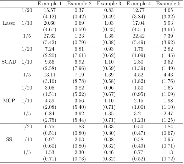
The results of sequential instability analysis show that with 5-fold CV, MCP and SCAD are more stable than Lasso except for the highly correlated covariates case of Example 2 and the low dimensional Example 3. In Example 1, when only 5% of the data are removed, Lasso would choose a model with more than 15 terms different on average.
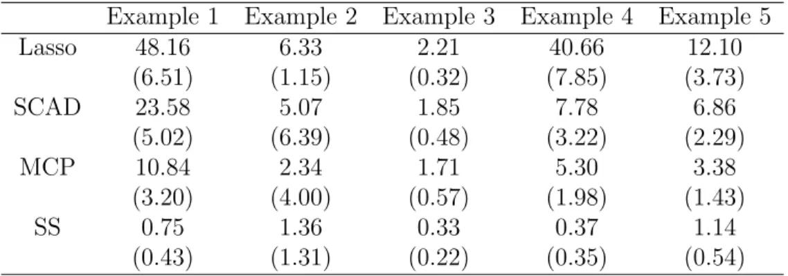
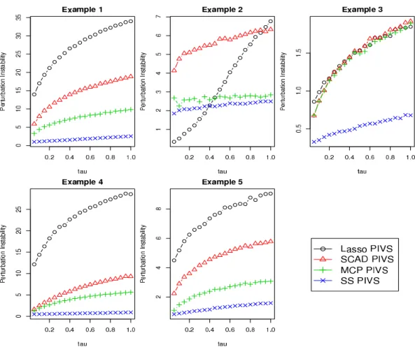
Table Table 2.2 is the result of bootstrap instability analysis. Lasso displays the largest bootstrap instability for all the data sets. The perturbation instability is given in Figure Figure 2.1. All the penalization procedures display increasing trends in the perturbation instability, as expected. The comparison between the selection procedures is somewhat similar to that of the sequential instability.
Table 2.1: Sequential Instability
Example 1 Example 2 Example 3 Example 4 Example 5
1/20 15.57 0.37 0.83 12.77 4.65 (4.12) (0.42) (0.49) (3.84) (3.32) Lasso 1/10 20.60 0.69 1.03 17.04 5.93 (4.67) (0.59) (0.43) (4.51) (3.61) 1/5 27.62 1.23 1.35 22.42 7.39 (5.42) (0.79) (0.38) (5.49) (3.92) 1/20 7.24 6.81 0.93 1.76 2.82 (2.20) (7.61) (0.62) (1.09) (1.45) SCAD 1/10 9.56 6.92 1.10 2.80 3.52 (2.58) (7.96) (0.59) (1.39) (1.49) 1/5 13.11 7.19 1.39 4.52 4.43 (3.16) (8.78) (0.58) (1.82) (1.76) 1/20 3.05 3.82 0.96 1.50 1.65 (1.51) (5.22) (0.67) (0.95) (1.09) MCP 1/10 4.59 3.56 1.10 2.15 1.98 (2.08) (5.40) (0.71) (1.00) (1.10) 1/5 6.84 3.92 1.35 3.21 2.47 (2.75) (5.44) (0.71) (1.23) (1.25) 1/20 0.75 1.83 0.33 0.50 0.84 (0.51) (0.80) (0.30) (0.47) (0.67) SS 1/10 0.97 2.03 0.38 0.58 0.95 (0.60) (0.80) (0.32) (0.49) (0.71) 1/5 1.53 2.30 0.46 0.77 1.13 (0.71) (0.73) (0.32) (0.52) (0.72)
From the results on SIVS, PBIVS and PIVS, we see that for some cases, the insta-bilities of the methods are reasonably small, but in other cases, they are unacceptably high. Take Lasso on Example 1, for instance. With parametric bootstrap, on average, the bootstrap data give a set of predictors that differs from the original selection by over 40 terms, and even at τ near 0, the perturbation instability of the 5-fold CV based Lasso is very high. If one is to use Lasso for variable selection here, a different tuning than 5-fold CV is needed. Note that the Stability Selection is confirmed to be very stable, with much smaller values of SIVS, PBIVS, and PIVS (except Example 2)
Table 2.2: Parametric Bootstrap Instability
Example 1 Example 2 Example 3 Example 4 Example 5
Lasso 48.16 6.33 2.21 40.66 12.10 (6.51) (1.15) (0.32) (7.85) (3.73) SCAD 23.58 5.07 1.85 7.78 6.86 (5.02) (6.39) (0.48) (3.22) (2.29) MCP 10.84 2.34 1.71 5.30 3.38 (3.20) (4.00) (0.57) (1.98) (1.43) SS 0.75 1.36 0.33 0.37 1.14 (0.43) (1.31) (0.22) (0.35) (0.54)
compared to the other methods. The price paid by SS for stability is its larger ten-dency to ignore true predictors when the noise level is not low. The detailed results under the three instability measures are provided in a supplementary file Additional Numerical Results.
2.4.3
VSD
We demonstrate the performance of the VSD on Lasso, SCAD, MCP, Stability Selec-tion and a forward selecSelec-tion. For the forward selecSelec-tion (FS), one predictor is added sequentially and the model with the smallest value of a modified BIC (see below) is selected. The five simulation examples with different noise level σ varying from 0.01 to 30 are examined. We simulate 100 data sets for each example. The base model
m0 for each of Lasso, SCAD and MCP is the selected model based on the value of
λ corresponding to the smallest 5-fold cross validation error. The Bayesian informa-tion criterion is modified by taking into account both the model complexity and the dimensionality:
BIC0 =nlog(ˆσk2) +rklog(n)−2ψlog(πk),
Figure 2.1: Perturbation Instability
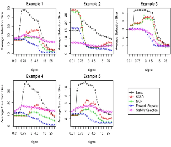
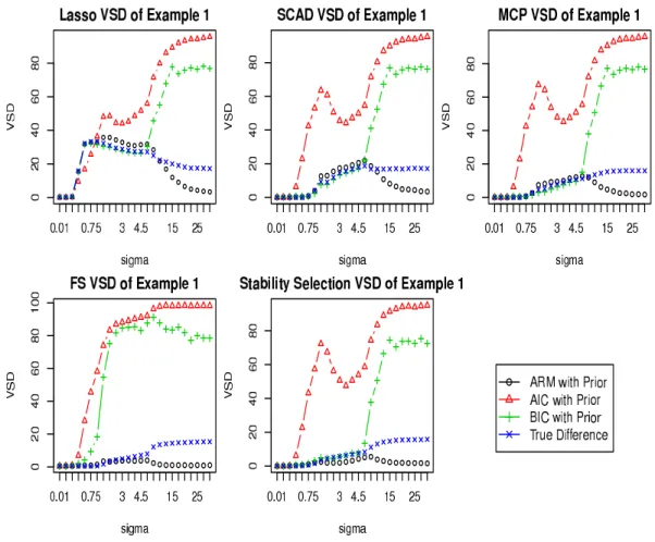
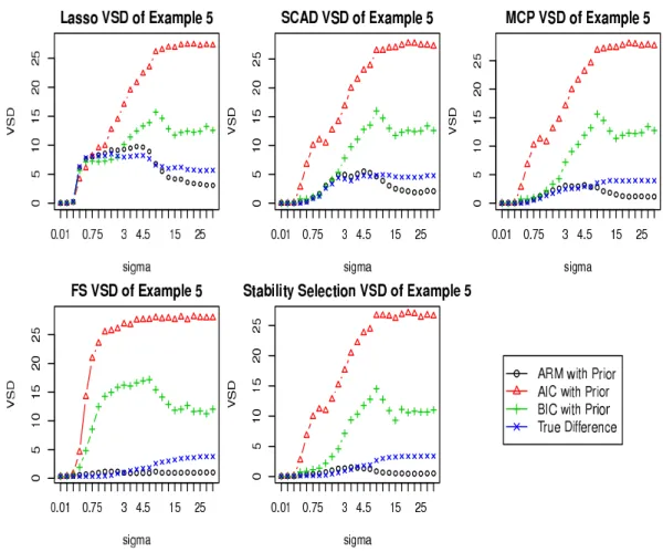
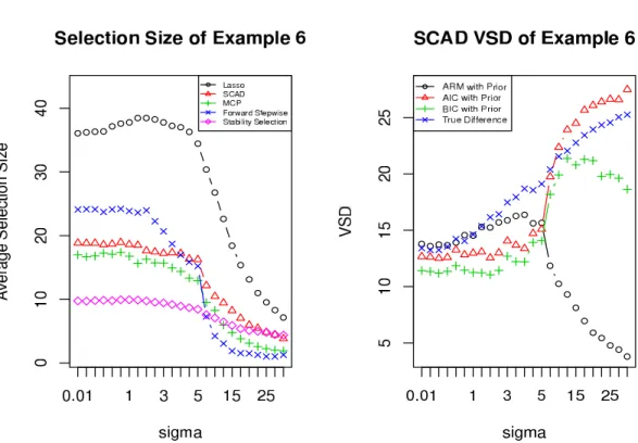
Figure Figure 2.2 summarizes the average selection size of the model selection procedures at different variance levels. The average selection size eventually decreases for all of them (but at different paces) as the variance level increases, as expected. The VSD graphs for the examples are in Figures Figure 2.3-Figure 2.7.
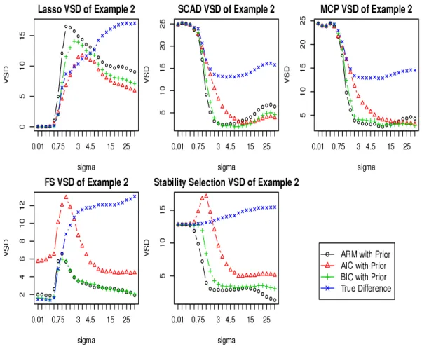
When the predictors have a grouping structure (Example 2), SCAD and MCP select a large number of variables at small variance levels, but SS selects too few predictors. In contrast, the selected model sizes of FS and Lasso are good. In the other examples, FS and SS basically have the same pattern in terms of the selection size as the noise level increases.
Figure 2.2: Average Selection Size withψ = 1
The selected model sizes for Lasso, SCAD and MCP are not monotone in noise level, different from what one would expect, when the true model size is smaller than
n/2. Except Examples 2 and 6, the selection sizes of Lasso, SCAD and MCP are close to the true model sizes at a low level of error variance, but they may increase first when the error variance is moderate and then decreases.
Example 6. There are 50 observations and 60 predictors, 10 with coefficient 1, 9 with coefficient 2.5, and 7 with coefficient 5. The positions of the true predictors are randomly selected. The pairwise correlation between xi and xj isρ|i−j| with ρ= 0.3.
Figure 2.3: VSD for Example 1 with ψ = 1
The selection size and the VSD of the non-sparse example are illustrated by SCAD in Figure Figure 2.8.
The VSD graphs are very interesting.
1. When the true model size is small and σ is relatively not large, we see that the VSD values based on ARM with a non-uniform prior are quite close to the true sizes of the symmetric difference between the true model and the selected model in terms of variable composition. In such a case, the VSD provides a sensible understanding on how much the selected model deviates from the truth. When
σgets very large, we see that the true deviation size and the VSD values diverge: the former tends to increase and the latter tends to decrease. This is expected
Figure 2.4: VSD for Example 2 with ψ = 1
and cannot be avoided because, as the signal to noise ratio decreases to zero, any sensible model selection method chooses fewer and fewer terms. This is also related to explaining why we see that when σ is very small or very large, the VSD values are small. They are so for different reasons: when σ is very small, the VSD is small due to that the identified model is close to the true model; whenσ is very large, the selected model is very small and the weighting cannot support the true model due to extreme lack of information and consequently concentrates on very small models as well. In any event, a large value of the VSD relative to the size of the selected model does indicate that the selected model is unreliable with the deviation size roughly given.
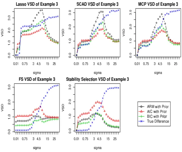
Figure 2.5: VSD for Example 3 with ψ = 1
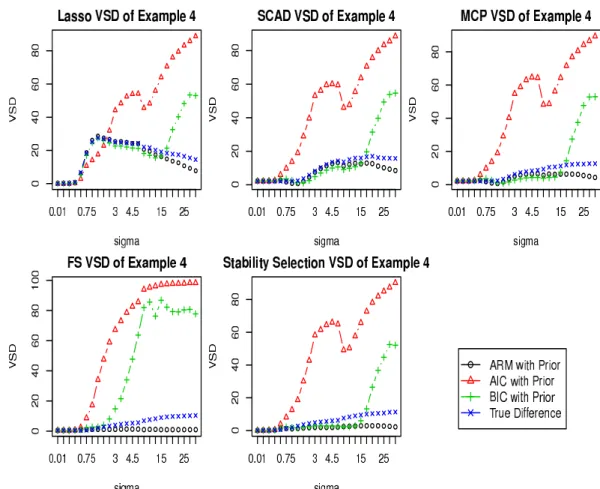
2. The prior weight on the models is very important. Without the prior, all of the weighting methods, ARM, AIC and BIC perform very poorly for the purpose of measuring the deviation of interest (the results are not presented here or in the supplementary file). With the prior added, both ARM and BIC perform quite well, although BIC has some troubles for Examples 1, 4 and 5. It turns out that for these cases, if the constant ψ is enlarged to e.g. 2.5, then (the modified) BIC can be much improved. For ARM, in Examples 2 and 3, whenσ
is in a small window in the middle, its VSD values are somewhat larger than the actual deviation and thus the ARM weighting can be a little exaggerating about unreliability of the selected model. Based on our investigations, it seems fair to
Figure 2.6: VSD for Example 4 with ψ = 1
say that for the purpose of identifying important variables, the AIC weighting (with or without the prior) is unsatisfactory for the VSD.
3. Not surprisingly, none of the model selection methods dominated others. With 5-fold CV, Lasso is often more prone to over-fitting. But in Example 2, it per-formed mostly better than SCAD, MCP and SS, which had a major challenge. The forward selection performed similarly to Lasso in that case.
4. Comparing Example 3 with Example 5, we see somewhat unusual behaviors. For the simpler situation with only 8 predictors, for the low noise cases, Lasso, SCAD and MCP all over-fit, but to different degrees (roughly by 2, 0.5 and
Figure 2.7: VSD for Example 5 with ψ = 1
0.5 terms, respectively on average). Interestingly, when 52 noise variables are added to the predictors, under very low noise, the over-fitting tendencies are perfectly curtailed. However, when the noise level is not too small, we clearly see the harm of having irrelevant predictors in data.
5. From the VSD values, we see that the sparse patterns identified by the model selection procedures have drastically different reliabilities, some being strong T-sparsity and some others being severe F-sparsity. For instance, for Example 1, at σ = 1.5, Lasso gives an F-sparsity, but for Example 2 with σ = 0.5, both SCAD and MCP give unreliable F-sparsity.
Figure 2.8: Selection size and VSD of SCAD for Example 6 withψ = 1
6. Another confirmative observation is that the correct choice of a model size does not mean a good choice of predictors. For instance, in Example 2, when σ is about 1, the average model sizes selected by SCAD and MCP are both close to the true model size. However, from the VSD plots, we see that the VSD values calculated by the BIC weighting with a prior are around 19. In fact, V SD+ and V SD− are 8 and 11, respectively, indicating that the two methods have difficulties in both type I and type II directions.
7. When the size of the true model is even larger than half the sample size (Example 6 in Figure Figure 2.8), we see that the selection becomes extremely difficult even at very smallσvalues. The VSD values properly reflect the true departure of the selected model by SCAD from the true model when the error variance is small. Whenσ is larger, we see a new pattern compared to the other examples: while the ARM–based VSD substantially under-estimates the target, BIC– and
AIC–based values are much closer. The reason is that with the true model so complex relative to the sample size, the cross-validated weights in ARM strongly favor very simple models. The over-estimation tendencies of BIC- and AIC–based VSD values seen in some earlier examples of sparse situations now become actually beneficial.
The VSD results are shown in Figure 4 - 9. When the dimension is moderate, all weight function except AIC yield satisfactory performance with the differ-ence between the true model size and selection size. It can be seen that in the case of high dimension (Example 1, 5 , and 6), all information criterion VSD are increasing with the variance. The MARM and MARM with prior weight functions calculate similar VSD for forward stepwise selection, and the MARM with prior for Lasso and SCAD captures the difference between the true model size and the selection size. However, when the dimension is small (Example 4), the MARM and AIC weight functions yield almost the same VSD. On aver-age, BIC and BIC with prior weight function perform better than others when the variance is small, in terms of captures the deviation from the true model size; While MARM and AIC weight functions beat other weight function if the variance is large.
2.4.4
Real Data
Huang et al. (2008) apply the adaptive Lasso on the data set reported in Scheetz et al. (2006). Here we use this data set to illustrate the application of the VSD in high dimensional regression. In the data, 120 twelve-week-old male offsprings generated from an F1 animals intercross were selected for tissue harvested from eyes. The microarrays contain over 31042 probe sets. The gene expression values are log transformed.
We follow the steps in Huang et al. (2008) to include probes expressed in the eye or with sufficient variation and there are 18976 such probes. The interest is to find the genes related to the gene TRIM32. We thus perform a regression of the probe 1389163 at (from TRIM32) on the remaining 18975 probes to find out the genes that are strongly related with TRIM32.
After a screen as done in Huang et al. (2008) (the issue of possible screening bias is not addressed in this work), we have 120 rats and 200 probes. We first examine the instabilities of the model selection methods on this data set. For SS, the threshold probability is set at 0.6. When 5% of observations are removed, the SIVS of Lasso, SCAD, MCP, SS, and FS are 8.1, 9.32, 3.54, 1.62 and 1.76, respectively, and the corresponding PBIVS values are 23.09, 11.79, 3.81, 0.99 and 0.97. The PIVS values of 5-fold CV Lasso are also rather large.
The results of the VSD analysis are shown in Table Table 2.3. Lasso selected many more probes than the others. Similarly to the simulation results, AIC with the non-uniform prior does not seem to provide helpful information on variable selection uncertainty. Both ARM and BIC, with the active prior, give more or less the same picture. With the limited information, relying on the weighting by BIC or ARM, we see that all the model selection methods perhaps have chosen more variables than strongly supported by the weights at the current sample size, to different degrees (e.g., 18 terms for Lasso as seen in the V SD− values).
The weighting of ARM and BIC support only around 3 predictors (other than the intercept). Although some other genes may have potential values in prediction, from the perspective of identifying the most important predictors with reliability, the methods of Lasso and SCAD have selected variables that are not quite justified at the current sample size. We run the LS regression on the chosen predictors for each method. Based on the standard outputs of the linear regression, we see that only 1 out of 20 (non-constant) terms are significant at the 0.05 level for Lasso, and the ratio is
Table 2.3: VSD of Microarray Analysis
Lasso SCAD MCP FS SS (threshold=0.6)
Selection Size 20 12 4 3 3
ARM with prior 18.64 10.66 2.85 1.82 5.27 VSD AIC with prior 26.46 18.96 15.88 16.75 20.25
BIC with prior 18.47 10.25 1.70 3.53 7.61 ARM with prior 0.47 0.48 0.58 0.56 2.27
V SD+ AIC with prior 12.10 12.35 14.82 15.75 17.50 BIC with prior 1.54 1.43 1.15 2.57 4.61 ARM with prior 18.17 10.18 2.27 1.27 3.00
V SD− AIC with prior 14.35 6.60 1.07 1.00 2.75 BIC with prior 16.93 8.82 0.54 0.96 3.00
5/12 for SCAD, 4/4 for MCP and 3/3 for the forward selection. Even if their selected predictors had been given a prior (rather than selected from out of 200 choices), one probably needs to agree that the 5-fold CV based Lasso and SCAD have selected too many predictors. The outcome that the weighting of ARM and BIC support a model of size only around 3 may seem to be too conservative. But given that the variables are selected from many genes, it perhaps can be argued that the weightings are doing the right thing. Keeping in mind the sentiment by some biologists that the important genes picked up by machine learning methods are frequently not confirmed in later costly experiments, together with our earlier simulation results, we believe that the use of the VSD measures can help safeguard against over-selection in the pool of a huge number of predictors.
Coefficient estimation from LS
forward coefficient
Estimate Std. Error t value Pr(>|t|) (Intercept) 5.66584 0.18276 31.002 < 2e-16 *** 1383110_at 0.11204 0.03394 3.301 0.00128 **
1383996_at 0.14089 0.02657 5.302 5.53e-07 *** 1389584_at 0.16546 0.03225 5.130 1.17e-06 ***
Lasso Coefficient
Estimate Std. Error t value Pr(>|t|) (Intercept) 6.261e+00 6.114e-01 10.240 <2e-16 *** 1369353_at -2.063e-02 5.563e-02 -0.371 0.712 1370429_at 1.492e-02 5.466e-02 0.273 0.785 1371242_at -3.510e-02 5.054e-02 -0.694 0.489 1374106_at 3.656e-02 5.881e-02 0.622 0.536 1374131_at 2.007e-02 3.139e-02 0.639 0.524 1378935_at -1.504e-02 4.404e-02 -0.342 0.733 1379971_at 4.193e-02 6.157e-02 0.681 0.497 1380033_at 3.741e-02 2.976e-02 1.257 0.212 1381787_at -9.425e-03 6.291e-02 -0.150 0.881 1382835_at 5.645e-02 3.522e-02 1.603 0.112 1383110_at -2.790e-04 4.808e-02 -0.006 0.995 1383522_at 1.584e-02 3.681e-02 0.430 0.668 1383673_at 5.988e-03 5.100e-02 0.117 0.907 1383749_at -4.440e-02 3.693e-02 -1.202 0.232 1383996_at 8.838e-02 3.453e-02 2.560 0.012 * 1389584_at 4.740e-02 4.877e-02 0.972 0.333 1390788_a_at 2.194e-02 4.122e-02 0.532 0.596 1393382_at 1.500e-02 3.718e-02 0.403 0.688 1393684_at 1.083e-02 2.731e-02 0.397 0.692 1393979_at -1.324e-06 5.232e-02 0.000 1.000
SCAD Coefficient
Estimate Std. Error t value Pr(>|t|) (Intercept) 6.5656082 0.4516868 14.536 < 2e-16 *** 1368923_at -0.0097362 0.0436837 -0.223 0.824058 1371242_at -0.0521217 0.0506233 -1.030 0.305541 1374106_at 0.0876848 0.0344749 2.543 0.012420 * 1374131_at 0.0585856 0.0279937 2.093 0.038753 * 1378935_at -0.0410461 0.0383180 -1.071 0.286514 1380033_at 0.0293750 0.0270175 1.087 0.279388 1383749_at -0.0354301 0.0305261 -1.161 0.248391 1383996_at 0.1062684 0.0266834 3.983 0.000125 *** 1384305_at -0.0005703 0.0427943 -0.013 0.989393 1389584_at 0.1584874 0.0413281 3.835 0.000214 *** 1393684_at 0.0339757 0.0225248 1.508 0.134435 1394107_at -0.1204826 0.0338661 -3.558 0.000561 *** MCP Coefficient
Estimate Std. Error t value Pr(>|t|) (Intercept) 6.22311 0.31405 19.815 < 2e-16 *** 1374106_at 0.10548 0.03223 3.273 0.001406 ** 1383996_at 0.13100 0.02524 5.191 9.13e-07 *** 1384305_at -0.07957 0.02303 -3.455 0.000772 *** 1389584_at 0.14921 0.03031 4.923 2.87e-06 ***
The V SD+ and V SD− values also provide very useful information. From
Ta-ble TaTa-ble 2.3, based on the ARM weighting (with a non-uniform prior), Lasso, MCP and SCAD have missed at most 1 detectable gene and SS may have missed up to 3 genes. The V SD− values in Table Table 2.3 suggest that Lasso and SCAD have
chosen quite a few genes that are hard to justify at the current sample size.
With the 5-fold tuning, in this example, Lasso selected a model of size much larger than those by the other methods (more than seen in the simulations). We suspect that this may be related to complicated correlations between the predictors. Indeed, from the sample correlation matrix of the variables selected by Lasso, for each of them, four excepted, there is at least one pairwise correlation around 0.7 or higher with some other variables, even up to 0.9. The high correlations perhaps confused Lasso. We mention that Lasso and adaptive Lasso in Huang et al. (2008) selected 24 and 19 probes respectively.
To have a focused illustration, we have used the same 5-fold CV for tuning all the three penalized regression methods. Obviously Lasso and SCAD can be tuned to be much more parsimonious, and their behaviors in terms of the VSD measures can be very different from what are seen in this chapter. It is also possible that the different methods may need different ways of tuning to achieve their respective best performance, which is beyond the scope of this work.
We also performed a guided simulation study, using each of the originally chosen models by Lasso, SCAD, MCP and SS respectively to generate data.
2.4.5
Simulation Based on the Real Data
We perform a simulation study using the real data in section 4.4. We keep the original predictor values, but for each subject, the response ˜y is generated from N(ˆy,ˆσ2), where ˆy and ˆσ2 are the LS fitted value and the estimated standard deviation from the sparse regression model chosen by a specific method. By this way, based on the originally chosen model by Lasso, SCAD, MCP and SS respectively, 100 data sets are generated. The averages of the selected model size and the VSD measures for the model selection methods are given in Table Table 2.4 from the 100 simulation runs. The standard errors of these averages (not reported due to space limitation)
are mostly below 5% of the means.
Table 2.4: Simulation Study of Microarray Analysis
Lasso SCAD MCP SS
Lasso (size = 22)
Selection Size 22.66 8.14 4.94 3.17 True Difference 29.20 22.54 21.28 23.43 ARM with prior VSD 21.23 7.53 3.63 4.97 AIC with prior VSD 43.30 44.87 45.99 49.24 BIC with prior VSD 18.61 5.48 3.38 7.19
SCAD (size = 12)
Selection Size 23.29 8.30 5.57 2.99 True Difference 23.29 12.52 11.21 13.23 ARM with prior VSD 21.07 6.56 3.73 4.41 AIC with prior VSD 39.80 43.42 44.44 48.71 BIC with prior VSD 18.53 4.93 3.24 7.46
MCP (size = 4)
Selection Size 19.74 7.68 4.61 3.01 True Difference 17.06 6.22 3.71 6.13 ARM with prior VSD 17.78 6.08 2.97 4.34 AIC with prior VSD 43.73 45.74 47.23 50.85 BIC with prior VSD 16.26 4.92 2.64 6.30
SS (size = 3)
Selection Size 13.00 5.54 3.40 3.37 True Difference 10.32 3.92 2.86 0.87 ARM with prior VSD 11.79 4.52 2.31 2.86 AIC with prior VSD 65.46 69.63 70.62 71.09 BIC with prior VSD 10.58 3.65 1.92 2.92
The results, given in the supplementary file Additional Numerical Results, are very informative. We see that none of the methods really adapts to the true data generating model (DGM) in terms of the average selected model size. When the DGM is large (by using the Lasso model), all the methods are performing very poorly: the number of missed or falsely included predictors, on average, totaled to the true model size (or larger). Much more seriously, even when the true model is chosen to be small (by MCP or SS), all the methods are still not doing well: from the VSD values, they could not identify the true set of predictors reasonably closely. This seems to be due to the complicated correlations between the predictors. Indeed, from the sample correlation matrix of the variables originally selected by Lasso, for each of them, four
excepted, there is at least one pairwise correlation around 0.7 or higher with some other variables, even up to 0.9. Thus our simulation convincingly (hopefully) shows that high correlations of the gene expressions make the problem of identifying the “right” genes for a response variable extremely difficult.
As for the performance of the VSD, when the true model size is relatively large, the VSD values are quite good to describe the behavior of Lasso but are substantially smaller than the true difference sizes for the more parsimonious methods (again, because of very limited information, in presence of many weak coefficients and high correlations, any weighting cannot be expected to be around the true model). When the true model size is small (by MCP and SS), the VSD values properly indicate how many terms are questionable in the models chosen by the four methods. This real data guided simulation seems to support the finding from the VSD values based on the original data: the predictors selected by the penalization methods are mostly unreliable (due to the nature of the data).
2.5
Summary and Discussion
Penalized regression procedures aim to discover useful sparse patterns in high dimen-sional regression. Our numerical results demonstrated again that these methods can sometimes be quite unstable. To provide more information on reliability of a selected sparse pattern, we have introduced the concept of variable selection deviation (VSD) to measure the uncertainty of the selection in terms of inclusion of predictors in the model.
The Stability Selection improves the existing model selection method and gives a stable set of variables, which does not depend on the size of penalization parameters. Based on our study, by setting the threshold value to 0.9, the selected set is very stable, except the grouping structure case. Furthermore, the selection size pattern of
the Stability Selection is very similar to the forward selection with modified BIC. The VSD measures based on the ARM and BIC weighting with the non-uniform prior can be very helpful in pointing out how many important variables are possibly missed and how many are unnecessary in the selected model. Clearly, VSD measures are relative to the weighting assignment, and they can only quantify deviations from the models supported by the weights. Fortunately, we have seen that under the ARM weighting, for noise level not too high, the VSD values are very close or reasonably close to the actual deviation size between the true model and selected model and hence provide quite useful information on reliability of the selected model. When the noise level is high, without additional information, it is not possible to reliably find the true model. Any sensible weighting on the models needs to necessarily concentrate on models of small sizes that only keep the most important terms (or even none). In such a case, the VSD measures would be small, which are addressing the selection of the best model for prediction instead of the true model.
For ARM weighting, we chose the half-half data splitting. As shown in Yang (2001), this gives the best rate of convergence offered by the candidate regression procedures (not necessarily parametric) in terms of estimating the regression function. When comparing a fixed list of models/methods with the worse ones converging at a rate slower than 1/nunder the squared L2 loss for estimating the regression function, the results of Yang (2007a) (see the proof of Theorem 1 there) suggest that the half-half splitting would lead to a consistent weighting. A rigorous theoretical investigation is needed to understand when the ARM method yields a weakly consistent weighting for high-dimensional regression.
Another comment is on the use of CV for tuning parameter selection. Based on our simulations, 5-fold CV sometimes performs much better than 10-fold CV for the purpose of model identification (which is perhaps expected based on the work of Shao (1993) and Yang (2007a)).
Model selection diagnostics are severely missing both in research and application. Suitable model selection diagnostics measures can much improve quality of decisions based on statistical data analysis. For instance, if a biologist is to decide which genes to investigate in expensive and time consuming confirmatory study based on an exploratory data analysis, the VSD measures may honestly tell that the majority of the genes recommended by a method may not be as promising as the selected model suggests.
VSD in Generalized Linear Model
3.1
Introduction
The Generalized linear model (GLM) is a standard framework for modeling the asso-ciation between a continuous/discrete response and a set of independent variables. In modern research and application areas, often a large number of predictors are used to classify the response variable into several categories. For example, the target of the genome wide association studies is to identify a subset of single-nucleotide polymor-phisms (SNPs) that are associated with human diseases over thousands of SNPs (Wu et al. (2009)). In such cases, it is challenging and difficult in the variable selection and the coefficient estimation to use the traditional methods, such as AIC (Akaike (1973)), BIC (Schwarz (1978)) and Cp (Mallows (1973)), due to heavy computation
demand.
Assume that a random sample ofnsubjects{(yi,xi), i= 1,· · · , n}is observed. Let
Yi be a response variable following a distribution in the exponential familyf(yi;θi) =
exp[yiθi−A(θi) + B(yi)], where θi is the parameter and µi = E(Yi) = A0(θi). Let
Xj ∈Rn, j = 1, . . . , p be p predictors. The usual GLM framework models the mean µi of Yi via the link function transformation
g(µi) = β0+βiXi1+· · ·+βpXip.
A variety of exponential distributions (i.e. in McCullagh and Nelder (1989)) can be modeled with different link functions, such as the identity link for Gaussian regression, the logit link log1−prpr =g(µ) for logistic regression where the binary response follows a binomial distribution Bin(n, pr), and the log link for Poisson regression where the response is from a Poisson distribution.
In recent years, the penalization method, an effective and computationally feasible approach, has been well developed to perform the variable selection and parameter estimation. The penalized likelihood estimator is solved by following objective func-tion: ˆ βλ = arg min ( `n(β) + p X j=1 p(|βj|;λ) ) ,
where `n=Pni=1[yiθ(Xi, β)−A(θ(Xi, β))] and p(|βj|;λ) is the penalty function with
a tuning parameterλ.Tibshirani (1996) introduced anL1 penalty for variables called Lasso. Zhao and Yu (2006) and Zou (2006) proved the inconsistency of Lasso for model selection in certain scenarios. Fan and Li (2001) proposed SCAD, which is a non-concave penalized likelihood method. Zou (2006) proposed the adaptive Lasso, which modified Lasso penalty to guarantee the selection consistency. Zhang (2010) proposed a minimax concave penalty (MCP) and developed a fast penalized linear unbiased selection algorithm. The results of penalization methods heavily depend on the amount of regularization. Therefore, choosing a proper amount of regularization is critical. On the other hand, the theoretical results of penalization methods are usually derived under the assumption of sparsity. Sometimes, the assumption is not easy to justify. In particular, when the sample size is much smaller than the number predictors, sensible variable selection methods tend to select a sparse model. There-fore, we may question the reliability of the results of a penalization method. How much certainty do we have about the set of variables selected by the regularization method on the current data? Also, is the sparse pattern discovered by these variable
selection methods real?
In literature, the uncertainty of model selection methods has been well studied, such as Breiman (1996b), Yuan and Yang (2005), and Chen et al. (2007). When the dimensionality is large, we expect the instability of a model selection method to be high. Nan and Yang (2014) tested three instability measures for three penalization methods: Lasso, SCAD, and MCP in the context of linear regression. The results showed that these methods sometimes could be quite unstable. They also proposed a model selection diagnostic measure called variable selection deviation (VSD), which provides a proper sense on how many predictors in the selected set are likely trustwor-thy in certain aspects. Rather than focusing on the sense of instabilities of a model selection method, the VSD evaluates the reliability of a set of selected variables and captures the difference from the underlying true set of predictors.
In the generalized linear model context, the VSD measures also uses a weighting mechanism to help measure the deviation of the selected variables by a generalized linear model method from the true model, so that users will have a reasonable sense about the reliability of the set of selected variables. In this chapter, we extend the VSD measures from the linear regression setting to the generalized linear model, in particular, logistic regression. We also propose the weighting function for poisson regression, in order to demonstrate the implementation of the VSD measures to other generalized linear models.
The chapter is organized as follows. In Section 2, the theoretical results of the VSD for generalized linear model are proposed, and we also introduce the weight function for logistic regression and the corresponding algorithm. The numerical results of simulation studies and the studies of four real data examples are shown in Section 3.
3.2
Variable Selection Deviation
The variable selection deviation measures (VSD), proposed in Nan and Yang (2014), use an external information to evaluate the reliability of the given selected set of vari-ables derived from a model selection method. Therefore, users can have a reasonable sense on how trustworthy the identified model is.
Let ∆ = {mk, k ≥ 1} be a collection of candidate models for data Z = {Zi =
(xi, yi), i = 1, . . . , n}. Let m0 be the model that need to be examined, and m∗ be
the underlying true model with r∗ predictors. The VSD in Nan and Yang (2014) is defined as follows.
Definition 3
For a target modelm0, the VSD corresponding to a weightingwon the list of models ∆ is
V SD(m0) = V SD(m0;w; ∆;n) = X
mk∈∆
wk·#(mk∇m0),
where # denotes the cardinality set and∇ denotes the symmetric difference between two sets. The upper and lower VSD of m0 are defined as
V SD+(m0) = X mk∈∆ wk·#(mk\m0), and V SD−(m0) = X mk∈∆ wk·#(m0 \mk),
where mk\m0 refers to all the variables that are in model mk but not in m0.
Thus by weighting the target model m0 and a countable collection of candidate modelsmkin ∆,V SD(m0) measures the average size of deviation form0. V SD+(m0)
number of missing variables in m0. V SD−(m0) is the number of variables which are irrelevant and should not be included in the selection set.
Before presenting a theorem of the VSD measures in the generalized linear model context, we introduce definitions on the behavior of a model selection method. Given a positive constant J, let ∆J denote the subset of models in ∆ that each misses at
mostJ terms of the true modelm∗ and let ∆J denote the subset of models in ∆ that
each has at most J terms not in the true model m∗. Because m∗ is selected with a model selection method, we denote ˆm= ˆm(δ) as the model selected by a method δ.
Definition 4
A model selection method δ is weakly over-consistent if there exists a sequence of positive numbers Jn with Jn/r∗ →0 such that
P( ˆm(δ)⊆∆Jn)→1.
It is strongly under-consistent if there exists a constant 0< κ <1 such that
lim inf
n→∞ P( ˆm(δ)*∆κr
∗)>0.
It is strongly over-fitting if there exists a constant η >0 such that
lim inf
n→∞ P( ˆm(δ)*∆
ηr∗)>0.
The following result on the VSD measures holds.
Theorem 2
Suppose that the model weightingw is weakly consistent. 1. If δ is consistent in selection, then
2. If δ is weakly over-consistent in selection, then
V SD+(δ;w)/r∗ →0 in probability.
3. Ifδis strongly under-consistent in selection, thenV SD+(δ;w)/r∗does not converge to zero in probability.
4. If δ is strongly over-fitting in selection, then V SD−(δ;w)/r∗ does not converge to zero in probability.
5. The VSD is close to its target:
|V SD( ˆm)−#( ˆm∇m∗)|
r∗
p
→0.
Proof 3.1 (Proof of Theorem 2)
1. When δ is consistent, P( ˆm(δ) =m∗)→1. The conclusion follows readily since
w is weakly consistent.
2. Under the assumption that δis weakly over-consistent, there existsJnsuch that Jn/r∗ →0 and P( ˆm(δ)∈/ ∆Jn)→0. Since mk\mˆ(δ) is a subset of the union of mk\m∗ and m∗\mˆ(δ) for each mk, we have
X mk∈∆ wk#(mk\mˆ(δ))≤ X mk∈∆ wk#(mk\m∗) + X mk∈∆ wk#(m∗\mˆ(δ)). Therefore, X mk∈∆ wk#(mk\mˆ(δ))≤ X mk∈∆ wk#(mk\m∗) +Jn,
with probability approaching to 1. Together with that w is weakly consistent, the assertion follows.
3. Let Abe the event thatδselects a model with more thanκr∗ terms inm∗ miss-ing, for which lim infn→∞P(A)≥ >0 for some. Sincewis weakly consistent,
we must haveP mk∈∆κr∗ 2 wk →1 in probability. In eventA, #(mk\mˆ(δ))≥ κr ∗ 2 for mk in ∆κr∗
![中文文字蘊涵系統之特徵分析 (Feature Analysis of Chinese Textual Entailment System) [In Chinese]](data:image/gif;base64,R0lGODlhAQABAIAAAP///wAAACH5BAEAAAAALAAAAAABAAEAAAICRAEAOw==)