Novel QoS-Aware Proactive Spectrum
Access Techniques for Cognitive
Radio Using Machine Learning
METIN OZTURK 1, MUHAMMAD AKRAM2, SAJJAD HUSSAIN 1,
AND MUHAMMAD ALI IMRAN 1, (Senior Member, IEEE)
1School of Engineering, University of Glasgow, Glasgow G12 8QQ, U.K.
2Department of Electrical Engineering, University of Engineering and Technology, Faisalabad Campus, Lahore 38000, Pakistan
Corresponding author: Metin Ozturk ([email protected])
This work was supported by the DARE Project through the Engineering and Physical Sciences Research Council U.K. Global Challenges Research Fund Allocation under Grant EP/P028764/1. The work of M. Ozturk was supported by the Republic of Turkey Ministry of National Education under Grant MoNE-1416/YLSY.
ABSTRACT Traditional cognitive radio (CR) spectrum access techniques have been primitive and inefficient due to being blind to the occupancy conditions of the spectrum bands to be sensed. In addition, current spectrum access techniques are also unable to detect network changes or even consider the requirements of unlicensed users, leading to a poorer quality of service (QoS) and excessive latency. As user-specific approaches will play a key role in future wireless communication networks, the conventional CR spectrum access should also be updated in order to be more effective and agile. In this paper, a comprehensive and novel solution is proposed to decrease the sensing latency and to make the CR networks (CRNs) aware of unlicensed user requirements. As such, a proactive process with a novel QoS-based optimization phase is proposed, consisting of two different decision strategies. Initially, future traffic loads of the different radio access technologies (RATs), occupying different bands of the spectrum, are predicted using the artificial neu-ral networks (ANNs). Based on these predictions, two strategies are proposed. In the first one, which solely focuses on latency, a virtual wideband (WB) sensing approach is developed, where predicted relative traffic loads in WB are exploited to enable narrowband (NB) sensing. The second one, based onQ-learning, focuses not only on minimizing the sensing latency but also on satisfying other user requirements. The results reveal that the first strategy manages to significantly reduce the sensing latency of the random selection process by 59.6%, while theQ-learning assisted second strategy enhanced the full-satisfaction by up to 95.7%.
INDEX TERMS Cognitive radio networks, dynamic spectrum access, machine learning, self-organizing networks,Q-learning.
I. INTRODUCTION
The concept of Cognitive Radio (CR) has been proposed in 1999 [1] in order to use the electromagnetic frequency spectrum more efficiently. On one hand, some portions of the spectrum experience an over-utilization, making them scarce in bandwidth, while on the other hand, some other portions, such as the ones allocated by TV channels, may experience an under-utilization [2], [3], leading to network resource wastage. Mobile cellular networks, for example, are supposed to accommodate a growing number of users with increasing data traffic [4], albeit being bandwidth limited [5]. The associate editor coordinating the review of this manuscript and approving it for publication was Xijun Wang.
To mitigate the bandwidth scarcity in wireless communica-tion networks, two different types of users have been intro-duced in the CR concept:Primary User (PU)andSecondary User (SU). The former is a licensed user who always has priority to access the spectrum, while the latter is unlicensed and can use the spectrum opportunistically. Given that SUs utilize the vacant portions of the spectrum, this process not only improves the spectral efficiency, but also eases the con-gestion in the mobile cellular networks, especially in ultra-dense scenarios.
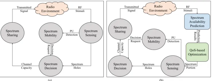
As shown in Fig. 1a, there are four phases included in the conventional CR spectrum access process: spectrum sensing,spectrum decision,spectrum sharing, andspectrum mobility[6]. In the spectrum sensing phase, SUs sense the
FIGURE 1. (a) Conventional and (b) proposed CR spectrum access processes. The proposed method puts two additional phases (WB spectrum prediction and QoS-based optimization) before sensing in order to enhance SU’s satisfaction by selecting the network that suits best with the requirements of SU.
spectrum continuously to find an idle channel to allocate. In the spectrum decision phase, SUs choose a channel to associate with (in case of multiple channels being available), while spectrum sharing refers to the process of sharing the available frequency band with other SUs. Finally, evacuating the allocated channel in the presence of any PU in order to avoid interference is called spectrum mobility [7].
In addition to these steps, CR spectrum sensing can be divided into two main categories according to the size of the bandwidth to be sensed, which are: narrowband (NB) sensing and wideband (WB) sensing. The former refers to the case when the bandwidth to be sensed is not larger than the coherence bandwidth of the channel, while the latter hap-pens when the sensed bandwidth is larger than the coherence bandwidth [8].
Many NB spectrum sensing methods, such as energy detector-based [9], cyclostationarity-based [10], matched-filtering [11], etc., have been proposed in the literature [12]. However, the main drawback of NB sensing is that the band-width to be sensed is limited, so is the spectral opportunity. As such, NB sensing methods have to compromise on the greater number of available bands by focusing on a certain bandwidth.
Furthermore, because direct integration of NB sensing methods with WB sensing is not possible due to their binary decision approaches [8], other methods, such as sub-Nyquist sensing [13], have been proposed for WB sensing. However, the WB sensing methods are often more complex to imple-ment [8], making them prone to higher latency due to long sensing time [13]. As latency is a key parameter to consider in future mobile networks, especially when SUs run real-time applications, a large amount of sensing attempts can result in SUs being unsatisfied. As such, in order to decrease the sensing latency, predictive spectrum sensing methods have
been proposed in the literature [7], [14]–[24]. The main idea behind these methods is to produce an interface between WB and NB sensing; this is done by predicting future occupancy states of spectrum bands in WB to enable NB sensing to focus only on the bands that are predicted to be available. However, these prediction-based methods are not a contender of existing sensing techniques, but rather complementary, as the predicted availabilities of spectrum bands are exploited before going through the conventional sensing process to reduce the sensing latency [7]. Intuitively, the number of required sensing attempts decays by decreasing the band-width of interest, which in turn reduces the resultant latency. Nonetheless, the methods employed in [7], [14]–[24] could be unrealistic, as they rely on specific assumptions, such as having historic data set on the occupancy of each individual channel. As such, these predictive sensing implementations seem to be impractical, since it is unlikely to have historic data set on occupancy states for each individual channel. In addition, even if the data set for each channel is available, such kind of implementation would be very costly in terms of both memory and energy consumption due to higher storing and processing requirements. Furthermore, most of the afore-mentioned works take merely the latency as a Quality-of-Service (QoS) parameter and ignore other SU requirements during the spectrum sensing phase.
In this study, as shown in Fig. 1b, we propose a novel spectrum access approach, which includes a virtual predic-tive WB spectrum sensing andQoS-based optimization, with the aim of increasing the satisfaction of SUs by meeting their user/application-specific requirements of latency, cov-erage, and bandwidth. In the virtual predictive WB sensing, instead of being interested in individual frequency channels, the traffic loads of the Radio Access Technologies (RATs) are considered as a whole for predictions, as this approach
necessitates significantly less memory and processing due to less amount of data to be handled. Moreover, it is more likely and easier to have historic traffic load data sets for RATs than occupancy states of individual channels, and thus the proposed virtual predictive WB sensing method makes the process more realistic and practical.
In the proposed QoS-based optimizationphase, two dif-ferent decision strategies are introduced. The first strategy, which will be called WB Predictive Sensing (WBPS) here-after, focuses only on the sensing latency as a QoS parameter. Particularly, the future traffic loads of the RATs, occupying different portions of the WB spectrum, are predicted. Then, the bandwidth of the RAT with the minimum relative traf-fic load is selected to be sensed with NB sensing; hence, the probability of finding a spectrum hole is boosted by narrowing down the WB spectrum to the less utilized portion. In this way, higher spectral opportunity of WB sensing and easy implementation of NB sensing are both exploited. In other words, given the aforementioned problems,WBPS is the upgraded and modified version of existing predictive spectrum sensing approaches.
The second strategy, which will be called Q-Learning Enabled WBPS (QWBPS) hereafter, is a novel and more robust approach, in which the decision process in WBPS
is consolidated by considering all the QoS requirements of SUs, such as latency, coverage and bandwidth. Since the proposed approach is not limited to these QoS parameters, any other user requirement can easily be appended to the model. Furthermore, the SUs are allowed to prioritize the QoS parameters, rendering the proposed algorithm capable of adapting itself to dynamically changing scenarios and circumstances.
Normally, running aQ-learning algorithm also takes some time, which may lead to an additional latency. However, the proposed framework is proactive and timing is not an issue, since the Q-learning implementation is performed in advance by predicting the future traffic loads. Additionally, as it will be elaborated in SectionV-B, since the proposed Artificial Neural Networks (ANN) algorithm is fed with time and day inputs, it is able to predict the traffic load not only for the next time slot but also for any given time and day.
However, despiteQWBPSbeing more robust and dynamic, it comes at the expense of more computational cost due to the additionalQ-learning implementation. In that regard, a trade-off arises, in which it is better to useWBPSif the latency is the only concern, whileQWBPSis a better choice in case the SU has additional concerns other than the latency.
The rest of the paper is organized as follows: SectionII summarizes the state-of-the-art on predictive CR manage-ment. Section IIIpresents the system model including the analytic derivations, and Section IV elaborates the data sets that are used to facilitate this work. Section V intro-duces the proposed methodology in a comprehensive manner. Section VI, first, provides detailed information about the implementation phase, then discusses the obtained results. Lastly, SectionVIIconcludes the paper.
II. RELATED WORK
Spectrum prediction has been extensively studied in the liter-ature by employing various techniques [7], such as Hidden Markov Model (HMM) [18], [22], ANN [14], [20], Long Short-Term Memory (LSTM) [17], Autoregressive (AR) model [19], etc. In [14] the authors tried to predict the future occupancy states of a channel by designing a Multi-Layer Perceptron (MLP) with backpropagation (BP). They generated a synthetic PU traffic for a single channel using Poisson process, while the channel’s ON/OFF times were determined using geometric distribution. It was observed that the spectrum utilization was boosted and that the sens-ing energy was decreased. An analytical model for SU’s throughput was derived in [15] by considering both the imperfect spectrum prediction and protection to PUs. Some numerical studies were also performed to observe how the SU’s throughput is affected by different parameters, such as prediction error and the number of channels to be sensed.
In [21] the performance of a BP ANN for spectrum pre-diction was improved by employing genetic algorithm at the training phase, as conventional BP ANN is very prone to be trapped into a local optimum [25]. An HMM based prediction of future states of a channel was presented in [16]. A channel selector, which includes a channel state predictor and a channel environment evaluator, was introduced so that the channel selection process becomes the combination of Signal-to-Interference-plus-Noise-Ratio (SINR) level and the availability of the channel. Another HMM based spectrum prediction is presented in [22], where real data was collected by measuring Wi-Fi signals via the experimental set-up with four different antennas.
An ALOHA system was assumed in [23], in which a second-order AR and Kalman filter were employed to predict occupancy states of the spectrum. A recent work in [24] stud-ied the predictive spectrum management in a comprehensive manner. First, SU’s mobility was predicted using second-order Markov model. Second, the spectrum prediction was also performed and combined with the mobility predictions. Finally, a channel selection phase was also executed in case of multiple channel availability. The authors also included a joint prediction cost model by considering the errors occur-ring at each stage.
Nevertheless, most of the predictive sensing works avail-able in the literature have been performed for a single (or a few) channel(s) scenario. This is not applicable for WB sensing albeit being practical for NB sensing, since it is not possible to predict the future occupancy levels of numerous frequency channels in WB. Furthermore, they [14], [16]–[18], [20], [22], [24] mostly rely on the availability of historic channel occupancy data sets for each individual channel, making them even more unrealistic, since it is hard to have such data sets for all channels at all possible locations and times. In addition, in such implementations, the memory and energy consumption increases with increasing bandwidth of interest (or number of channels), as more data will be
needed to conduct machine learning training for increased number of channels.
Furthermore, as most of the existing studies were per-formed using synthetically generated occupancy states; i.e. 1 is busy and 0 is free, they are yet to be tested in more complicated and realistic scenarios, where multiple channels are available with different characteristics and limitations. Therefore, there is a significant need for an implementa-tion of predictive spectrum management schemes in more complicated environments. In addition to the lack of real-istic implementations, none of the studies aforementioned considered QoS requirements of the SUs before proceeding to the sensing phase. As such, in this paper, we propose predicting the future traffic loads of RATs in WB instead of predicting the occupancy states of individual frequency channels, since it is easier to have/collect related data sets. Moreover, due to less data requirements, the proposed vir-tual predictive WB sensing method results in less mem-ory and energy consumptions. Besides, the requirements of SUs are also taken into consideration in order to augment their experienced QoS satisfaction. Lastly, prioritization of QoS parameters are also allowed to make the proposed frame-work more user/application-specific.
The main contributions of this paper are: 1) In order to make the model realistic:
• four different RATs with different frequency ranges are considered;
• a real data set from [26] is employed for RAT-I and RAT-II, which mimics GSM and LTE, respectively;
• RAT-III and RAT-IV are aimed to mimic IEEE 802.11n 5 GHz and IEEE 802.11n 2.4 GHz, respectively. The synthetic data generation for RAT-III and RAT-IV is inspired by the real data measurements from [27].
2) Since the data set in [26] consists of many squared grids, in order to avoid over-fitting as well as reducing computational cost, ak-means algorithm is employed to cluster the grids according to their traffic load characteristics.
3) Due to diversified characteristics of each assumed RAT, different ANN models are developed during future traf-fic load predictions.
4) Two different decision approaches (WBPS and
QWBPS) are proposed to satisfy user-specific require-ments. In particular, theWBPS approach is proposed for users with only latency concern, whileQWBPSis developed for users who have other QoS requirements in addition to latency. In WBPS, future traffic load predictions for the RATs are exploited to direct the SUs to the most available RAT for latency reduction purposes, while in QWBPS, future load predictions, QoS requirements, and QoS element weights are exploited in order to satisfy the requirements of the SUs by usingQ-learning.
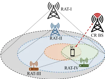
FIGURE 2. System model. An SU is surrounded by four different RATs. RAT-I, RAT-II, RAT-III, and RAT-IV are aimed to take the characteristics of GSM, LTE, IEEE 802.11n (5 GHz), and IEEE 802.11n (2.4 GHz), respectively. SU: Secondary User, CR BS: Cognitive Radio Base Station.
5) A weighting mechanism for QoS elements is developed to allow the SUs to prioritize their requirements. This enables the users to adjust their requirements for spe-cific applications, making the proposed method both user and application centric.
III. SYSTEM MODEL
As shown in Fig.2, the system model considers four RATs around an SU. There is also a CR Base Station (CR BS) that is responsible to provide coverage and data transmission for the SU. Therefore, the SU in this environment searches for an available frequency band to initiate its connection. Latency, coverage, and bandwidth are considered as QoS parameters in this study, and they will be detailed individually in the following paragraphs.
A. USER REQUIREMENTS
The coverage requirement refers to the distance that the SU will be away from its current location. If the SU is mobile, for example, then it will need an RAT offering more coverage in order for its connection to last longer. As shown in Fig.2, since RAT-I offers the widest coverage area, it would preferably be selected as an RAT to be sensed in the case of high mobility of the SU.
The bandwidth requirement, or data rate requirement, in this work reflects how much bandwidth the SU demands to run a desired application. In the case of video-conferencing, for instance, huge data rates are required; hence, an RAT with more available bandwidth is preferred.
Theorem 1: Let xf be a random variable that represents
full-satisfaction, where SU’s both coverage and bandwidth requirements are satisfied simultaneously, such that xf = 1
if full-satisfaction is achieved, and xf = 0otherwise. Then,
the expected value of full-satisfaction is E[xf]=
z
X
i=1
where pt,i is the probability of full-satisfaction for RAT i,
ps,iis the probability of selecting RAT i, and z is the number
of available RATs.
Proof: We first develop a random search concept for
benchmarking purposes. In this random search model, SUs first select a random RAT, after that channels in the frequency spectrum of the selected RAT are sensed in a random manner in order to find an available channel to occupy. Therefore, the RAT selection is a random process following the dis-crete uniform distribution. LetObe the set of the available RAT options:
O= {91, 92, ..., 9z}, (2) whose index set is
I= {1,2, ...,z}. (3) Let n ∼ U(1,z) be a random variable used to select the index of RAT to be sensed from I. Moreover, letps be the probability of being selected as an RAT to be sensed1:
ps = 1
z, (4)
wherez= |I|is the cardinality ofI. SU’s QoS requirements (R) are given as:
R=(Rc,Rb), (5)
whereRis a 2-tuple of coverage requirement,Rc ∈ N, and bandwidth requirement,Rb∈N.
Each RAT option can be equivalent to a tuple of its cover-age and bandwidth capabilities, respectively, such that
9i=(2c,i, 2b,i), ∀i∈I, (6) where 2c and 2b are the sets of coverage and bandwidth capabilities, and
2c=[2c,1, 2c,2, ..., 2c,z], (7) and
2b=[2b,1, 2b,2, ..., 2b,z]. (8)
pc,irepresents the probability of satisfying the SU’s cover-age requirement with RATi:
pc,i=P(2c,i≥Rc). (9)
Letxcbe a random variable that represents the coverage sat-isfaction, wherexc =1 if coverage satisfaction is achieved, andxc=0 otherwise. Then, the expected value of coverage satisfaction is E[xc]= z X i=1 pc,ips,i. (10)
pb,irepresents the probability of satisfying the SU’s band-width requirement with RATi:
pb,i=P(2b,i≥Rb). (11)
1Please refer to Table1for a glossary.
TABLE 1.Glossary.
Letxbbe a random variable representing the bandwidth sat-isfaction, wherexb=1 if bandwidth satisfaction is achieved, andxb = 0 otherwise. The expected value of bandwidth requirement becomes: E[xb]= z X i=1 pb,ips,i. (12)
Finally, the probability of full-satisfaction with RATiis the multiplication of satisfaction probabilities of both coverage and bandwidth requirements:
pt,i=pc,ipb,i. (13)
B. SENSING LATENCY
Latency in this work refers to the delay caused by unsuc-cessful sensing attempts, where the SU senses a frequency channel that is already being used by a PU. Another attempt with a different frequency channel is required after each
FIGURE 3. Milan city divided into square-shaped cells [26]. In this study, only the first 5,000 cells are considered (the lower half).
failure; hence, latency increases with the increasing number of failures.
Letpa,ibe the probability of finding a frequency hole with RATiin the first attempt:
pa,i=
Na,i
Nf,i
, (14)
where Na,i and Nf,i are the number of available channels and the total number of frequency channels for RAT i, respectively.
Therefore, it is obvious that a higher probability of finding an available channel is obtained when the total number of channels is small, which is the main idea behind the predictive sensing approach.
Letxa be a random variable that represents finding a fre-quency hole in a selected RAT, wherexa = 1 is frequency hole is found, andxa=0 otherwise. Then, the expected value becomes: E[xa]= 1 z z X i=1 Na,i Nf,i . (15)
IV. DATA SET & PREPROCESSING
There are two different data sets are employed in this work: Milan city data set [26] for RAT-I and RAT-II; synthetic data set, which is inspired by [27] during generation, for RAT-III and RAT-IV.
A. DATA SET FOR RAT-I AND RAT-II
Telecom Italia provides a data set belonging to Milan city for November and December 2013. In this data set, Milan city is divided into 10,000 square grids with a dimension of 235 meters. For each grid, aggregated call-in, call-out,
SMS-in, SMS-out, and internet activity levels have been recorded with 10 minutes resolution.
To use the data set in this study, we first combined call-inandcall-outactivities asCALL, andSMS-inandSMS-out
activities asSMS. Then, historic data set for RAT-I is created by combining CALL and SMS, while the internet activity
TABLE 2.User motifs for RAT-III and RAT-IV.
is treated as the historic data set for RAT-II. Due to some missing data and for the sake of computational efficiency, the first 5,000 cells and first 3 weeks of November data have been considered. The first two weeks of the three-week data set were used for training, while the remaining one week is used for testing.
B. DATA SET FOR RAT-III AND RAT-IV
Since RAT-III and RAT-IV are intended to mimic Wi-Fi networks, Wi-Fi related data set is required. As we do not have available data set for any Wi-Fi network, it is synthet-ically generated by being inspired by [27], in which real Wi-Fi data traffic was measured from 2147 wireless devices (196 residential gateways in 110 different cities) for 2 months. The primary objective of the work is to capture Wi-Fi usage patterns of the users. The authors extracted many user motifs (101 weekly motif and 112 daily motif), however 14 weekly motifs and 48 daily motifs have strong supports, meaning they are dominant over others [27].
In this study, two motifs are selected from [27] among the provided dominant ones, as shown in Table2, to generate our data set for RAT-III and RAT-IV, but the proposed study is not limited to any particular motif.
The synthetic data generation is carried out for 8 weeks, where 7-week data is used for training purposes while 1-week data is used for testing.
V. PROPOSED METHODOLOGY
In the traditional CR spectrum access process, SUs perform either NB sensing or WB sensing methods in order to find an available frequency band to allocate. Both have some certain advantages and disadvantages. In the NB sensing, for exam-ple, spectrum opportunities are limited with the narrower bandwidth of interest, leading to missing opportunities. In the WB sensing, on the other hand, albeit having more spectral opportunities, time spent for sensing is higher due to the larger amount of bandwidth to be sensed.
In this study, as shown in Fig. 1b, we propose a virtual WB sensing method, in which traffic load predictions for various RATs in WB are conducted in order to narrow down the band-width to be sensed, enabling NB sensing methods. In other words, NB sensing could be employed for the RAT, which is selected from WB using traffic load predictions. More par-ticularly, in case of multi-RAT availability, since each RAT may use different frequencies and bandwidth, the bandwidth-of-interest would most likely to be WB where NB sensing is no more applicable. In the proposed virtual WB sensing method, we choose an RAT out of all the available ones based
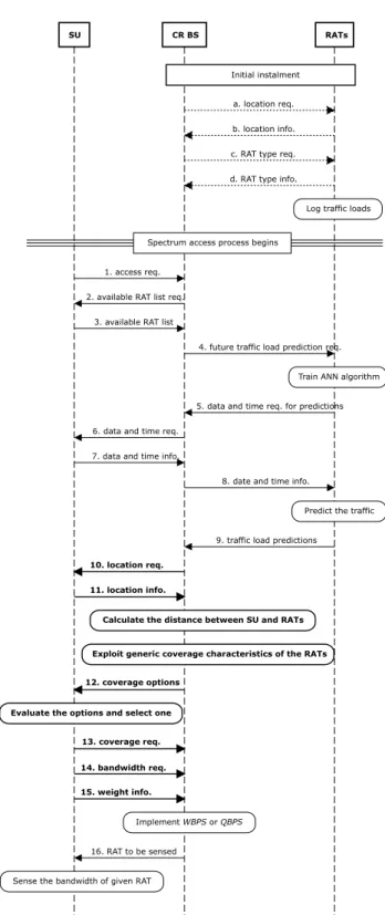
on traffic load predictions and/or user requirements, and the spectrum sensing procedure is performed to the bandwidth of the selected RAT. As such, the WB bandwidth-of-interest is narrowed to the bandwidth of the selected RAT, which in turn enables NB sensing approaches. Therefore, the proposed method uses the cooperation of WB and NB sensing by exploiting the inherent advantages of both methods. Note that the messaging between the SU, CR BS, and RATs are demonstrated in Fig. 4, which reveals how the proposed method might be implemented in real-life scenarios.
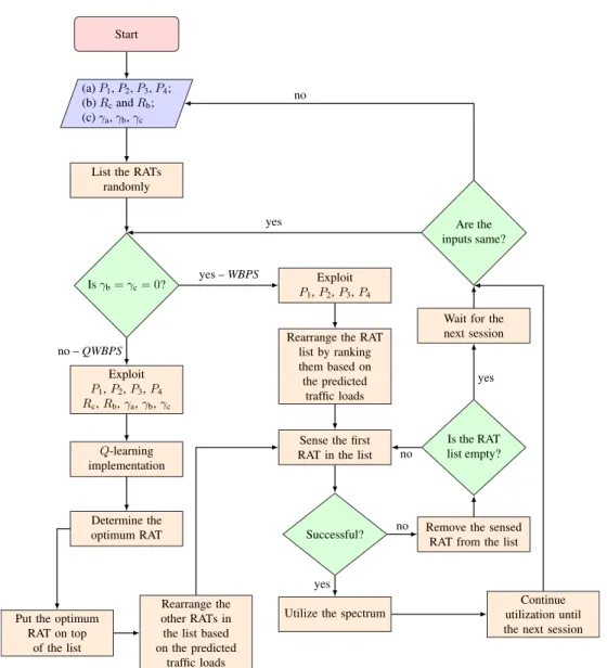
The second main contribution of the proposed method is to take the QoS requirements of the SUs into account, where the objective function is adjusted according to user-specific requirements with the help ofQ-learning. As shown in Fig.5, the proposedQoS-based optimizationphase consists of two different decision strategies:
1) WBPS: As shown in Figs. 4 and 5, at each ses-sion (instance), when the SU wants to access to the spectrum, the associated CR BS asks the RATs around the SU for future traffic load predictions. Then, the CR BS prepares an RAT list by ranking the RATs from min-imum to maxmin-imum according to their relative predicted traffic loads (percentage occupancy). Then, it directs the SU to the first RAT, whose traffic load is the mini-mum, to sense. If the SU cannot find a vacant channel in the selected RAT, it starts sensing the next RAT in the list, and this process continues until there is no RAT left to sense. If the SU cannot find a vacant channel in any available RAT, then it counts the session as a fail and waits for the next session. This method targets only the latency minimization using virtual WB sensing by making the bandwidth to be sensed narrower.
2) QWBPS: As a main contribution of this study, all the user requirements are taken into account in order to boost the satisfaction level of the SUs. We consider coverage and bandwidth requirements in addition to latency, but the proposed method is not limited to any specific requirement; any other requirement can easily be appended to the framework. As seen in Figs.4and5, the CR BS receives the coverage and bandwidth requirements of the SU along with the QoS weights as inputs, and executes Q-learning accordingly in order to determine the optimum RAT to sense. However, as Fig.5reveals, QWBPS switches toWBPSin case there is no frequency channel available in the deter-mined optimum RAT.
After including the QoS requirements, there are four different KPIs to be investigated: coverage-satisfaction, bandwidth-satisfaction, full-bandwidth-satisfaction, and sensing latency.
A. CLUSTERING FOR MILAN CITY DATA SET
Training a cell in Milan city data set individually is very prone to have an over-fitting problem, as there is a limited number of samples for each cell. Therefore, it is a better approach to train the cells together for a better generalization that can lead to better prediction performance, since many samples
FIGURE 4. Sequence diagram showing the messaging among SU, CR BS, and RATs for the proposed methodology. Steps a-d (dashed) take place in case of new CR BS and/or RAT BS installment. Steps 1-16 happen when the SU requests to initiate a connection. Steps 10-15 (bold) are executed only forQWBPS, while steps 1-9 and step 16 are executed for bothWBPS
andQWBPS.
from various cells will be digested during the training. On the other hand, training only one machine learning algorithm for all the cells decreases the prediction accuracy while keeping the algorithm well-generalized. In other words, the algorithm
FIGURE 5. Flowchart for the two proposed methods.P1,P2,P3,P4are the future traffic load predictions for RAT-I, RAT-II, RAT-III, and RAT-IV, respectively.RcandRbare the coverage and bandwidth requirements, respectively.γa,γb, andγcare prioritization coefficients for QoS parameters: Latency, bandwidth, and coverage,
respectively. In case the optimum RAT determined byQWBPSdoes not have any available frequency channel, the process switches toWBPS.
will try to obtain a model that somehow fits all the cells. Nonetheless, the model will be very unlikely to fit all the cells perfectly, as their characteristics are quite different from each other; for example, while some are located at the city center, some are at more rural areas. Thus, there exist a trade-off between having a good generalization and a good prediction accuracy. In this regard, clustering the cells based on their traffic loads can be an intelligent solution; the cells are clustered with their similar peers; hence, generalization can be provided by compromising less from the prediction accuracy, since there will be different model for each cluster, whose elements have similar characteristics.
In this study,k-means clustering is employed in order to cluster 5,000 cells according to their average traffic loads.
k-means is an algorithm attempting to discover k different
clusters in a data set with various samples iteratively. For each cluster there is a dedicated centroid [28], and the basic idea behind this algorithm is to place these centroids and associate the closest data points to them. In the learning phase, the places of the clusters are altered by the average value of the associated data points in order to find an optimum clustering. Determining the number of clusters is one of the main issues for clustering problems. Intuitively, small number of clusters give huge errors, while smaller errors can be obtained with larger number of clusters [29]. Note that the error fork-means clustering is defined as the Euclidean distance between the centroid and its associated data points:
J(cj)=
X
xi∈cj
where cj is centroid of the cluster j, j = 1,2, ..,k; xi,
i = 1,2, ...,m, is the data points in the cluster j; µj is the mean of the cluster j. In extreme cases, for example, if the number of clusters equals to 1, then all the samples will belong to the same cluster, making the error enormous. On the other hand, if the number of clusters equals to the number of samples, there will be no error at all as all the samples will be associated to a cluster [29].
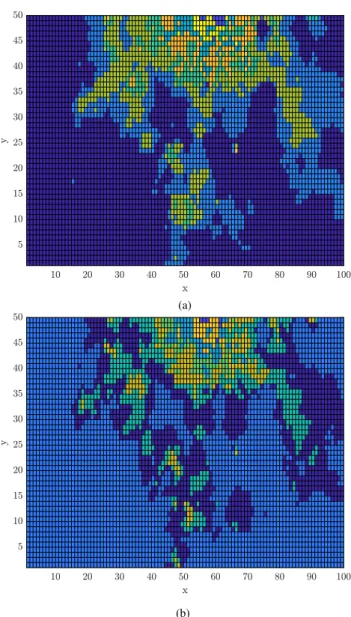
Thus, the elbow method [30] is used to find the optimum number of clusters by taking the percentage variation in the errors into consideration. Moreover, the stopping criteria for the employed elbow method is a 95% decrease in the error. In other words, first the initial error is calculated when the centroids are placed in a random manner, then the algorithm terminates whenever the 95% variation occurs in the obtained error. As such, the optimum number of clusters is found as 8 for the RAT-I, while it is 9 for RAT-II. The resulting clusters are shown in Fig.6.
B. FUTURE TRAFFIC LOAD PREDICTION
In order to predict the future traffic loads of each RAT, historic data is required to train the machine learning algorithms. For RAT-I and RAT-II, real telecom data set provided by Telecom Italia [26] for Milan city is used. For RAT-III and RAT-IV, the synthetic data set generation is inspired by [27], in which real Wi-Fi traffic was collected for 2-month period from 196 residential gateways.
1) ARTIFICIAL NEURAL NETWORKS (ANN)
ANN is selected as a supervised learning method due to its easy implementation and high performances [31]. Moreover, with being independent of information about the underlying distribution of the available data set in order to obtain a model, ANN outclasses statistical models [14].
Mean Squared Error (MSE) is used as a cost function for all the developed ANN models, in which the error is given by
CD=MSE= 1 m m X i=1 (yi−y0i)2, (17) wheremis the number of samples,yis the target value, and
y0is the predicted value.
The aim of the training phase is to minimizeCD in (17) by properly arranging weights and bias values. The Bayesian regularization [32] is employed as a training algorithm, since it is one of the strong BP training methods, preventing the network from over-fitting. More particularly, the Bayesian regularization introduces an extra parameter to the cost func-tion in (17):
C =αCD+βCW, (18)
whereCWis the cost implied by the ANN network weights, and α and β are the parameters to be determined. More specifically,CWis given by CW= 1 kwk X j=1 w2, (19)
wherewis the neural network weight vector.
FIGURE 6. Results of clustering the first 5,000 grids of the Milan city data set according to their average traffic load. (a) is for RAT-I, while (b) is RAT-II. Note that different colors represent different clusters, and the colors in (a) and (b) are independent from each other. Values inxandy
axes are for indexing purposes, and use (y−1)50+xto find the index of a particular grid. (a) Milan city map with clustering for RAT-I (k=8 clusters). (b) Milan city map with clustering for RAT-II (k=9 clusters).
In case α >> β, the training phase will prioritize the error reduction and will be prone to over-fitting. On the other hand, the training response will be well-generalized, but the obtained error will be higher in case of α << β [33]. Therefore, the trade-off inαandβ arises, and these param-eters need to be carefully tuned in order to minimizeCD as well as having a good level of generalization. In that regard, the Bayesian regularization with Lavenberg-Marquardt opti-mization, introduced in [33], is utilized in this work.
As there are four different RATs included in the proposed system model, the future traffic load predictions have been performed separately due to their distinctive characteristics. First, a fully-connected feed-forward ANN with input, hid-den, and output layers is employed for all the RATs as a
TABLE 3. Hyper-Parametrization for the different ANN models.
generic model. Then, the created generic model is customized individually for each RAT.
Determining the number of hidden layer (HL) neurons is an important issue in ANN, and some methods are recom-mended in [34] for this issue; however, they did not work well in our data sets, as all the methods suggest a small number of neurons which leads to under-fitting. Instead, an empir-ical approach is used to determine the optimal number of HL neurons. This approach considers gradually increasing the number of HL neurons starting from 1 to 20 in steps of 1 and evaluating the performance in terms of a cost function reflecting the obtained error.
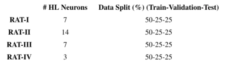
Similarly, an empirical method is followed in determining the data set split in terms of training, validation, and testing data. Basically, three different data splitting approaches are tested: 1) 50% training, 25% validation, 25% testing; 2) 60% training, 20% validation, 20% testing; and 3) 70% training, 15% validation, 15% testing. Then, based on the obtained hyper-parameterization results, different ANN models are developed for each RAT, as given in Table3.
After detailed hyper-parameterization analyses, number of HL neurons and data splitting, as in Table 3, are deter-mined for each RAT by considering the MSE performances of the ANN models. Significant MSE drop is investigated (mainly at least 95% drop is targeted) to select the number of HL neurons. After achieving at least 95% MSE drop, number of HL neurons are not increased even if it causes better MSE performance by considering the generalization of the model, since the more neurons included in the network, the model is more prone to over-fitting [35].
Similarly, 50-25-25 splitting is selected for all the ANN models, as there is no significant difference in terms of per-formance for the three data splitting approaches. The over-fitting problem is taken into account for this decision, since one of the reasons of over-fitting is over-training, leading to a lack of generalization of the developed ANN model [35].
a: ANN MODELS FOR RAT-I AND RAT-II
The input layer consists of 3 nodes: 1) indices of the grids; 2) days of the week; and 3) time of the day. In order to convert days of the week and time of the day into numeric values, they are encoded to linearly separated numbers betweenv1 = 0 andv2=1 with a spacing of
v2−v1
p , wherepis the number
of points. For the days of a week, linearly separatedp = 7 numbers generated between 0 and 1, and the days from Mon-day to SunMon-day are encoded to them respectively. Similarly, for
the time of a day, linearly separatedp = 144 numbers2are generated between 0 and 1, and times of a day are encoded to them accordingly. Only 1 output node, representing the data traffic loads, is included in the developed model for RAT-I and RAT-II.
b: ANN MODELS FOR RAT-III AND RAT-IV
Two neurons, which are days of a week and time of a day, are employed in the input layer. Moreover, the data encoding procedure conducted for RAT-I and RAT-II is adopted for RAT-III and RAT-IV, where days of a week are encoded to 7 linearly separated numbers between 0 and 1, and time of a day is encoded to linearly separated 144 numbers between 0 and 1. Similarly, there is only 1 neuron at the output for the data traffic loads of RAT-III and RAT-IV.
C. PROPOSED Q-LEARNING FRAMEWORK
As seen in Fig. 1b, the proposed method includes a pre-decision process where the portion of the spectrum (each RAT allocates different portions) to be sensed is determined based on either only the traffic load conditions (WBPS) or both the traffic load conditions and SU’s requirements (QWBPS).
WBPSrelies on the predicted availability of all the portions, and ranks them in terms of their relative traffic loads to select the most available one. InQWBPS, however, the pre-decision phase takes the requirements and associated weights from SUs into account in addition to the predicted traffic loads.
In order to accomplish this task, Q-learning [36] is employed. To solve this kind of optimum policy-seeking problems,Q-learning, which is one of the most outstanding reinforcement learning methods, is an important aspirant, since it is a model-free learning technique [37]–[39], which learns the environment by interacting with it.
There are six main components inQ-learning: (i) agent, (ii) environment, (iii) action, (iv) state, (v) reward/penalty, and (vi) action-value table. Agent takes actions by inter-acting with a given environment in order to maximize the reward or minimize the penalty. After each action that the agent takes, resulting state and reward/penalty are evaluated. Then, the action-value table, which stores the rewards/penalties for all the possible actions and states, are updated according to following rule:
Q(st,at):=Q(st,at)
+λ
Pt+1+φmin
a (Q(st+1,a))
−Q(st,at), (20) wherestandst+1are the current and next states, respectively.
Pt+1is the expected penalty for the next step andat is the action taken, whereais the set of all possible actions.λis a learning rate whileφis a discount factor.minfunction in (20) should be converted tomaxfunction to make the update pol-icy suitable for the reward-based framework, which includes a reward function instead ofP.
2The resolution of the data is 10 minutes, and there are 1440 minutes in a
TABLE 4. List of possible states and associated costs.
Q-learning is an off-policy method, meaning that it follows different policies in determining the next action and updating the action-value table. Although-greedy is the base policy,
πpolicy, where >0, is followed in selecting the next action, while µ policy, where = 0, is followed in updating the action-value table.
Three different states are designed in this work based on the satisfaction conditions of the user requirements. The states and associated costs to be incurred for being in the states are shown in Table 4. γc, γb, and γa in Table 4 are the prioritization weights for coverage, bandwidth, and latency, respectively, and the SU can tune them according to its pref-erences.εis the predicted occupancy level of the taken action.
ϕδ1 andϕδ2 are the costs of being inδ1andδ2, respectively, where ϕδ1 > ϕδ2, encouraging the agent to move to the best possible state. Hence, there is no such cost in δ3 as it is the best possible state.ζcis a cost function for the coverage requirement, where its value becomes 0 when the requirement is satisfied, and 1 otherwise
ζc=
(
0, 2c>Rc, 1, 2c<Rc,
(21) where2c is the coverage capability of the taken action and
Rcis the coverage requirement of the SU.
Similarly,ζbis a cost function for the bandwidth require-ment, where its value becomes 0 when the requirement is satisfied, and 1 otherwise
ζb=
(
0, 2b>Rb, 1, 2b<Rb,
(22) where2bis the available bandwidth in the action taken and
Rbis the bandwidth requirement of the SU.
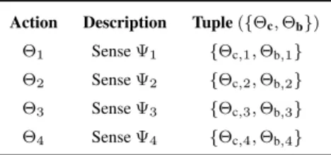
Furthermore, the action list is provided in Table5 where
2b,1,2b,2,2b,3, and2b,4 and2c,1,2c,2,2c,3, and2c,4 are the available bandwidth and coverage capabilities of RAT-I, RAT-II, RAT-III, and RAT-IV, respectively, where
2c,1> 2c,2> 2c,4> 2c,3. As seen from Table5, there are basically four different actions that the agent can perform, which correspond to the RATs that the agent can choose to sense.
In order to develop an optimization problem, we first define a global cost function as follows:
C(R, 9)=γcζc+γbζb+γad, (23) where d is the sensing latency, which can be modeled as
d = ε, since (14) implies that the probability of finding
TABLE 5.Q-Learning Action List.
a vacant frequency channel is directly proportional to the occupancy level of the spectrum. The lesser probability of finding a vacant frequency channel, the more sensing latency it causes.
Then, the optimization model becomes: min
n C(R, 9) (24a) s.t. 2c62mc, (24b)
2b62mb, (24c)
n6z, (24d)
where2mc and2mb are the maximum coverage and bandwidth supplies with the available RAT options.
Algorithm 1ProposedQ-Learning Algorithm Data: Predicted RAT traffic loads, SU requirements Result: RAT to be selected
1 forevery instancedo 2 InitializeQ(s,a):=0;
3 forepisodesdo
4 foriterationsdo
5 Determine the current state using Table4; 6 Take an action from Table5;
7 Calculate penalties through Table4; 8 Go to the next state;
9 Update theQ-table with (20).
10 end
11 end
12 end
Algorithm 1 summarizes the proposed Q-learning approach. In our implementation, SUs run this algorithm for each session and determine the best action to take.
The Q-learning algorithm allows the SUs to prioritize QoS components, which are coverage-satisfaction, bandwidth-satisfaction, full-bandwidth-satisfaction, and sensing latency. If, for example, the SU prioritize latency the most (e.g., running a real time application), then the algorithm attempts to mini-mize the number of unsuccessful sensing attempts, as it is the main reason for the delay in the spectrum sensing phase. In case the SU is mostly mobile, for instance, it would prior-itize the coverage requirement above all other components, as the RAT with the widest coverage area can keep the SU connected for a much longer time. Thus, the proposed
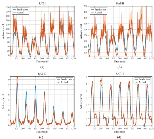
FIGURE 7. Future traffic load predictions for (a) RAT-I, (b) RAT-II, (c) RAT-III, and (d) RAT-IV. For (a) and (b), two weeks out of three weeks available data are used for training and one week is used for testing. For (c) and (d), seven out of eight weeks data are utilized for training purposes, while one week is used for testing. Note that the results are for a randomly selected cell. (a) Future traffic load prediction for RAT-I. (b) Future traffic load prediction for RAT-II. (c) Future traffic load prediction for RAT-III. (d) Future traffic load prediction for RAT-IV.
various requirements. In other words, the algorithm is able to adjust itself according to the preferences of SUs.
VI. PERFORMANCE EVALUATION
The model shown in Fig.2is used in this study to evaluate the proposed method. The network is monitored for a week with 10 minutes resolution. All the parameters utilized in the simulations are provided in Table6.
In the evaluations, the proposedWBPSandQWBPS meth-ods are compared with random RAT selection approach, where SUs first select a random RAT to sense, and then channels in the frequency spectrum of the selected RAT are sensed in a random manner in order to find an available channel to occupy.
The comparison is performed with the following metrics: (i) aggregated sensing latency, (ii) coverage satisfaction rate, (iii) bandwidth satisfaction rate, and (iv) full-satisfaction rate. The aggregated sensing latency represents the total latency incurred during the sensing phase in a week. Note that as the sensing latency has a strong correlation with the num-ber of unsuccessful sensing attempts, it is assumed that an unsuccessful sensing attempt causes a unit time (ut) of delay. The coverage and bandwidth satisfaction rates imply the
percentage of instances in one week3that the coverage and bandwidth requirements are satisfied, respectively. The full-satisfaction rate, on the other hand, represents the percentage of instances that both coverage and bandwidth requirements are satisfied simultaneously.
Since the existing predictive sensing methods, where the occupancy states of individual frequency channels are pre-dicted, are conceptually different from the proposed meth-ods, it is impossible to use them for comparison purposes. As aforementioned, the proposed WBPS and QWBPS are more realistic and implementable for WB sensing. Moreover, the QoS requirements of SUs are also taken into consideration
withQWBPS.
Fig. 7 shows sample traffic load predictions for RAT-I, RAT-II, RAT-III, and RAT-IV, respectively, for a random cell from a random cluster with 70-100 cells. The reason for putting this limitation to the cluster selection is just to make sure the cluster has sufficient number of elements for training while keeping it reasonable in order to avoid huge computa-tional cost. Results reveal that the proposed ANN manage to fit the data well, making the further phases implementable,
3an instance represents a 10 minute slot in a week simulation period. There
TABLE 6. Simulation parameters.
FIGURE 8. For various traffic levels, sensing latency performances of
WBPSand random search for finding one frequency channel. The sensing latency is directly correlated to the number of unsuccessful sensing attempts, and it is assumed that an unsuccessful sensing attempt takes one unit time (ut) of delay. Note that the results are the average of 100 runs.
since both pre-decision strategies (WBPSandQWBPS) use this predicted data as an input. Thus, any significant error that occurs in this prediction phase can lead to massive errors at the output.
Fig. 8 demonstrates the obtained sensing latencies for
WBPSand the random search for various data traffic levels. The purpose of this result is to reveal the behaviors of the random search and WBPS under different congestion lev-els, which is modeled by the data traffic loads; the more data traffic load an RAT experiences, the more congested
it becomes. In particular, the data traffic load for each RAT is varied from 10% to 1000% — by assuming the available traffic is 100% — in order to obtain various data traffic loads (or congestion levels). As shown in Fig.8, for the random search case, the obtained sensing latency increases tremen-dously when the congestion level becomes higher. Referring to the analytic model given in (15), the reason behind this result is that it is less likely to find a frequency hole to utilize when the network is more congested, leading to increasing number of unsuccessful attempts that causes increasing sens-ing latency. On the other hand, the senssens-ing latency gradually grows for various congestion levels if WBPS is used as a search strategy. Furthermore, WBPS decreases the latency significantly (up to 85.25% when traffic load is 500%) by always choosing the RAT whose relative traffic load is the minimum to sense. As such, it can clearly be seen that the probability of finding a vacant frequency channel is enhanced byWBPS, as it focuses its sensing on the least utilized portion of the available spectrum.
Fig.9 shows the percentage satisfaction rate of the SU’s coverage requirement. TheQWBPSstrategy managed to sat-isfy the SU at almost all the instances (99% success), while
WBPSand random search satisfied the SU for around 546.7 (54.24% success) and 631.9 (62.69% success) times on aver-age, respectively. These results also prove the superiority of
QWBPS; it can focus on the SU’s requirements and produce the output accordingly. The reason whyQWBPS could not give 100% success in satisfying the coverage requirement is that there are cases where there is no vacant channel in the RAT that is selected byQWBPS. As seen in Fig.5that
QWBPSswitches to WBPS in these cases, meaning that it
starts focusing on the sensing latency instead of any ment. Random search has no intention to satisfy the require-ments, thus the obtained results are,not surprisingly, the out-come of the random process. Appendix A demonstrates the calculations for coverage satisfaction of the random search using the model presented in SectionIII-A. As seen from the calculations in Appendix A and Fig.9, the analytic model in SectionIII-Aand the simulations are in line with each other, since the obtained results are very close.
Besides, the WBPS strategy does not have any aim of satisfying the user requirements as well. However, the reason why it produced worse results than the random search is that it always focuses on the option which relatively has the most available resources. As the RAT-III and RAT-IV, whose coverage capabilities are weak, mostly happened to offer the most relative resources,WBPStends to select these options.
Fig. 10 demonstrates the results for the satisfaction level in terms of bandwidth requirements. As seen from Fig.10,QWBPS(97.27% success) outperformed both ran-dom search (65.1% success) andWBPS(77.83%) by 49% and 25%, respectively. Note that the bandwidth requirement is prioritized for theQWBPScase; hence, it is able to increase the satisfaction level of the SU to a high level. There could be two different reasons explaining whyQWBPScould not give a 100% success rate: 1) OnceQWBPSswitches toWBPS
FIGURE 9. Percentage of coverage satisfaction for three different methods. The network is monitored for one week with 10-minute resolution. For theQ-learning part,γa=γb=0 andγc=5. Note that the obtained results are the averages of 100 runs.
when there is no available channel in the first selected RAT, the only focus becomes the sensing latency rather than spe-cific requirements. 2) The RAT determination is performed based on the predicted values, and there are some improper predictions, as seen in Fig.7, affecting the performance in a negative way. However, given thatQWBPSperformed quite well (97.27% success), these two issues are not problem-atic for the proposed methodology. On the other hand, it is interesting that WBPS gives better results than the random search, since there is no specific intention for that in the
WBPSstrategy. The main reason behind this outcome is that there is a strong correlation between minimizing the number of unsuccessful sensing attempts and the bandwidth require-ments, as the RAT option, which has the least occupancy level, is likely to have sufficient bandwidth.
Furthermore, the result for the random search case (65.1% success) is not surprising, and it is the outcome of the random process similar to the results in Fig.9. Appendix B provides the calculations for bandwidth satisfaction of the random search using the model presented in SectionIII-A.
The full-satisfaction levels for three different strategies are shown in Fig. 9, where coverage and bandwidth require-ments are equally prioritized for theQWBPScase. The results shown in Fig. 11a reveal thatQWBPSwas able to enhance the full-satisfaction ofWBPS and the random search by 95.7% and 83.8%, respectively, when sensing latency was not prior-itized along with the coverage and bandwidth requirements. On the other hand, QWBPSdid not perform well in terms of the sensing latency, as it reduced the sensing latency of the random search only by 8.96%, whileWBPSdecreased it by 60.2%. Given that coverage and bandwidth requirements were prioritized equally and no priority was given to the
FIGURE 10. Percentage of bandwidth satisfaction for three different methods. The network is monitored for one week with 10-minute resolution. For theQ-learning part,γa=γc=0 andγb=5. Note
that the obtained results are the averages of 100 runs.
sensing latency, these results also prove thatQWBPSworks very well according to the priority inputs, since it gave quite good results in terms of the full-satisfaction and performed poorly in the sensing latency.
In Fig. 11b, where the sensing latency, coverage and band-width requirements were all equally prioritized, it is demon-strated that the full-satisfaction level of QWBPS decayed by 16.3%, while the sensing latency performance was improved by 47.8%. Compared to the results in Fig. 11a, when all the parameters (sensing latency, coverage and bandwidth requirements) were equally prioritized,QWBPS
needed to compromise on the full-satisfaction to some extent in order to decrease the sensing latency. On one hand,QWBPS
boosted the full-satisfaction ofWBPSand the random search by 54.1% and 64.1%, respectively, while on the other hand, it managed to decrease the sensing latency of the random search by 52%. Furthermore, the difference betweenQWBPS
and WBPS in terms of the sensing latency declined from 56.3% to 17.3%. These results affirm the superiority of
QWBPSover the other methods, since it is capable of finding a good trade-off between the full-satisfaction and the sensing latency.
The full-satisfaction results of the random search is again the outcome of the random process, as in Figs. 9 and 10. If (1) and (13) are used with (27) and (28), the expected value for the random search to satisfy both the requirements simultaneously becomes 0.3287. The results also prove that Theorem 1 works properly.
Note that although the results in Figs.8, 9, 10, and 11 would be different for various simulation setups, such as different number of channels, different data rates, differ-ent RAT types, etc., they simply demonstrate the proof of
FIGURE 11. Results for sensing latency and the number of fully satisfied instances, which occurs when both coverage and bandwidth
requirements are satisfied simultaneously. The sensing latency is directly correlated to the number of unsuccessful sensing attempts, and it is assumed that an unsuccessful sensing attempt takes one unit time (ut). The network is monitored for one week with 10-minute resolution. Note that the results are the average of 100 runs. (a) Full-satisfaction and sensing latency whenγb=γc=5 andγa=0. (b) Full-satisfaction and sensing latency whenγa=γb=γc=5.
concept forWBPSandQWBPS. All these results reveal that the QWBPS strategy is more versatile thanWBPS, since it is capable of adjusting itself to the user requirements. Put it another way,QWBPScan be similar toWBPSwhen only the sensing latency is prioritized. However, it has much more capabilities thanWBPS. In other words,WBPScan be said to be a subset ofQWBPS, since it is only one task thatQWBPS
can do. In this regard, QWBPS approach is very strong, dynamic, and versatile, as it can easily adapt itself to different scenarios.
However, the power of QWBPS is at the expense of computational complexity, as it includes Q-learning in
addition to the processes performed inWBPS. Therefore, it is quite important to select either WBPSor QWBPS, and the selection should be application-specific. If the application is latency-intolerant and does not give importance to other QoS parameters, then there is no sense to use QWBPS, which is computationally more demanding. More particu-larly, QWBPS should be an option if the SU has multiple requirements.
VII. CONCLUSION
In this paper, we proposed a novel and comprehensive vir-tual predictive WB sensing approach with QoS-optimization phase. The proposed virtual WB sensing approach introduces an intelligent interface between WB and NB sensing methods by benefiting from both. Moreover, it does not suffer from huge memory and energy consumption problems as the exist-ing predictive sensexist-ing methods, since it treats the bandwidth of an RAT as a whole, which in turn reduces the amount of data to be handled.
In the QoS-optimization phase, two different decision strategies are proposed: the first one,WBPS, focuses only on minimizing the sensing latency, while the second strategy,
QWBPS, also considers user satisfaction. Both strategies have different purposes and they managed to fulfill their tasks successfully. Particularly, if the latency is the only concern for a given application,WBPSshould be selected as a strat-egy, since it merely focuses on reducing the sensing latency. Moreover, it is computationally less expensive thanQWBPS, as there is noQ-learning included in its process. Nonetheless, if the user has multiple requirements, then the choice should beQWBPSdue to its strong intelligent multi-objective opti-mization capabilities, which come at the expense of compu-tational complexity.
In future, we plan to extend this current work further by considering the cases where no historic dataset is avail-able, since this work relies on the assumption that there is already a historic data set that enables the proposed ANN,
k-means, andQ-learning algorithms to work. However, it is quite unlikely to have a data set for all locations and times. Furthermore, we also plan to add mobility to this current work by introducing a predictive mobility management, where the future locations of the users can be predicted in advance.
APPENDIX A
RANDOM SEARCH IN COVERAGE SATISFACTION Since there are four RAT options considered, (2) becomes
O= {91, 92, 93, 94}. (25)
In addition, it is assumed that SU’s coverage requirement is within the range of2c, such that
Therefore,E[pc] for this scenario becomes 0.625 using (10), where pc,i = 1.00 i=1, 0.75 i=2, 0.50 i=3, 0.25 i=4. (27)
If the SU chooses RAT-I, its coverage requirement will definitely be satisfied, as RAT-I’s coverage capability is the greatest of all the options in (25) and the assumption in (26) ensures that the SU cannot require more than available in2c. Furthermore, as the process follows the discrete uni-form distribution,ps,i=0.25, i= {1,2,3,4}.
APPENDIX B
RANDOM SEARCH IN BANDWIDTH SATISFACTION Using (25), and (28), the expected value in (12) is calculated as 0.655, which is in line with the result of 0.651 in Fig.10. In our implementations, Rb = τω, where τ represents 200 kHz bandwidth, andωis a coefficient determining the number of 200 kHz bandwidth that the user requires. ω follows the discrete uniform distribution between 1 and 20,
U ∼ [1,20], and the average probabilities of satisfying
Rb for RAT-I, RAT-II, RAT-III, and RAT-IV are evaluated through (11) as follows by calculating the average number of availableτ values for each:
pb,i= 0.4 i=1, 0.22 i=2, 1.00 i=3, 1.00 i=4. (28) REFERENCES
[1] J. Mitola and G. Q. Maguire, ‘‘Cognitive radio: Making software radios more personal,’’IEEE Pers. Commun., vol. 6, no. 4, pp. 13–18, Aug. 1999. [2] Y.-C. Liang, K.-C. Chen, G. Y. Li, and P. Mahonen, ‘‘Cognitive radio net-working and communications: An overview,’’IEEE Trans. Veh. Technol., vol. 60, no. 7, pp. 3386–3407, Sep. 2011.
[3] D. Datla, A. M. Wyglinski, and G. J. Minden, ‘‘A spectrum surveying framework for dynamic spectrum access networks,’’IEEE Trans. Veh. Technol., vol. 58, no. 8, pp. 4158–4168, Oct. 2009.
[4] Ericson Mobility Report, World Economic Forum, Ericson, Stockholm, Sweden, Jan. 2019.
[5] A. Gupta and R. K. Jha, ‘‘A survey of 5G network: Architecture and emerging technologies,’’IEEE Access, vol. 3, pp. 1206–1232, 2015. [6] I. F. Akyildiz, W.-Y. Lee, M. C. Vuran, and S. Mohanty, ‘‘A survey
on spectrum management in cognitive radio networks,’’ IEEE Commun. Mag., vol. 46, no. 4, pp. 40–48, Apr. 2008. [Online]. Available: https://ieeexplore.ieee.org/abstract/document/4481339. doi:
10.1109/MCOM.2008.4481339.
[7] X. Xing, T. Jing, W. Cheng, Y. Huo, and X. Cheng, ‘‘Spectrum prediction in cognitive radio networks,’’IEEE Wireless Commun., vol. 20, no. 2, pp. 90–96, Apr. 2013.
[8] H. Sun, A. Nallanathan, C.-X. Wang, and Y. Chen, ‘‘Wideband spectrum sensing for cognitive radio networks: A survey,’’IEEE Wireless Commun., vol. 20, no. 2, pp. 74–81, Apr. 2013.
[9] G. Yang, J. Wang, J. Luo, O. Y. Wen, H. Li, Q. Li, and S. Li, ‘‘Cooperative spectrum sensing in heterogeneous cognitive radio networks based on normalized energy detection,’’IEEE Trans. Veh. Technol., vol. 65, no. 3, pp. 1452–1463, Mar. 2016.
[10] M. Hejazi and B. Abolhassani, ‘‘Cyclostationarity-based multi-antenna cooperative spectrum sensing in cognitive radio networks over correlated fading channels,’’ inProc. Iranian Conf. Electr. Eng. (ICEE), May 2018, pp. 627–632.
[11] S. Dannana, B. P. Chapa, and G. S. Rao, ‘‘Spectrum sensing for fading wireless channel using matched filter,’’ inSoft Computing for Problem Solving (Advances in Intelligent Systems and Computing), vol. 817, J. Bansal, K. Das, A. Nagar, K. Deep, and A. Ojha, Eds. Singapore: Springer, 2019. [Online]. Available: https://link. springer.com/chapter/10.1007/978-981-13-1595-4_27. doi: 10.1007/978-981-13-1595-4_27.
[12] T. Yucek and H. Arslan, ‘‘A survey of spectrum sensing algorithms for cognitive radio applications,’’IEEE Commun. Surveys Tuts., vol. 11, no. 1, pp. 116–130, 1st Quart., 2009.
[13] Y. Ma, Y. Gao, A. Cavallaro, C. G. Parini, W. Zhang, and Y.-C. Liang, ‘‘Sparsity independent sub-Nyquist rate wideband spectrum sensing on real-time TV white space,’’IEEE Trans. Veh. Technol., vol. 66, no. 10, pp. 8784–8794, Oct. 2017.
[14] V. K. Tumuluru, P. Wang, and D. Niyato, ‘‘A neural network based spec-trum prediction scheme for cognitive radio,’’ inProc. IEEE Int. Conf. Commun., May 2010, pp. 1–5.
[15] J. Yang and H. Zhao, ‘‘Enhanced throughput of cognitive radio networks by imperfect spectrum prediction,’’IEEE Commun. Lett., vol. 19, no. 10, pp. 1738–1741, Oct. 2015.
[16] C.-H. Park, S.-W. Kim, S.-M. Lim, and M.-S. Song, ‘‘HMM based channel status predictor for cognitive radio,’’ inProc. Asia–Pacific Microw. Conf, Dec. 2007, pp. 1–4.
[17] P. Zuo, X. Wang, W. Linghu, R. Sun, T. Peng, and W. Wang, ‘‘Prediction-based spectrum access optimization in cognitive radio networks,’’ inProc. IEEE 29th Annu. Int. Symp. Personal, Indoor Mobile Radio Commun. (PIMRC), Sep. 2018, pp. 1–7.
[18] H. Eltom, S. Kandeepan, Y.-C. Liang, and R. J. Evans, ‘‘Cooperative soft fusion for HMM-based spectrum occupancy prediction,’’IEEE Commun. Lett., vol. 22, no. 10, pp. 2144–2147, Oct. 2018.
[19] A. Eltholth, ‘‘Forward backward autoregressive spectrum prediction scheme in cognitive radio systems,’’ inProc. 9th Int. Conf. Signal Process. Commun. Syst. (ICSPCS), Dec. 2015, pp. 1–5.
[20] S. Jain, A. Goel, and P. Arora, ‘‘Spectrum prediction using time delay neural network in cognitive radio network,’’ in Smart Innova-tions in Communication and Computational Sciences(Advances in Intel-ligent Systems and Computing), vol. 851, S. Tiwari, M. Trivedi, K. Mishra, A. Misra, and K. Kumar, Eds. Singapore: Springer, 2019. [Online]. Available: https://link.springer.com/chapter/10.1007/978-981-13-2414-7_25. doi:10.1007/978-981-13-2414-7_25.
[21] J. Yang, H. Zhao, and X. Chen, ‘‘Genetic algorithm optimized training for neural network spectrum prediction,’’ inProc. 2nd IEEE Int. Conf. Comput. Commun. (ICCC), Oct. 2016, pp. 2949–2954.
[22] Z. Chen, N. Guo, Z. Hu, and R. C. Qiu, ‘‘Channel state prediction in cog-nitive radio, part II: Single-user prediction,’’ inProc. IEEE Southeastcon, Mar. 2011, pp. 50–54.
[23] Z. Wen, T. Luo, W. Xiang, S. Majhi, and Y. Ma, ‘‘Autoregressive spectrum hole prediction model for cognitive radio systems,’’ inProc. IEEE Int. Conf. Commun. Workshops (ICC), May 2008, pp. 154–157.
[24] Y. Zhao, Z. Hong, Y. Luo, G. Wang, and L. Pu, ‘‘Prediction-based spectrum management in cognitive radio networks,’’IEEE Syst. J., vol. 12, no. 4, pp. 3303–3314, Dec. 2018.
[25] X. Sun, G. Gui, Y. Li, R. P. Liu, and Y. An, ‘‘ResInNet: A novel deep neural network with feature reuse for Internet of Things,’’IEEE Internet Things J., vol. 6, no. 1, pp. 679–691, Feb. 2019.
[26] Dandelion API, Open Big Data. Accessed: Jan. 4, 2019. [Online]. Avail-able: https://dandelion.eu/datamine/open-big-data/
[27] K. Mirylenka, V. Christophides, T. Palpanas, I. Pefkianakis, and M. May, ‘‘Characterizing home device usage from wireless traffic time series,’’ in Proc. 19th Int. Conf. Extending Database Technol.(EDBT), Mar. 2016, pp. 539–550.
[28] H. Xiong, J. Wu, and J. Chen, ‘‘κ-means clustering versus validation mea-sures: A data-distribution perspective,’’IEEE Trans. Syst., Man, Cybern. B. Cybern., vol. 39, no. 2, pp. 318–331, Apr. 2009.
[29] A. K. Jain, ‘‘Data clustering: 50 years beyond K-means,’’Pattern Recognit. Lett., vol. 31, no. 8, pp. 651–666, Jun. 2010.
[30] D. J. Ketchen and C. L. Shook, ‘‘The application of cluster analysis in strategic management research: An analysis and critique,’’Strategic Manage. J., vol. 17, no. 6, pp. 441–458, Jun. 1996.
[31] M. Ozturk, P. V. Klaine, and M. A. Imran, ‘‘Introducing a novel minimum accuracy concept for predictive mobility management schemes,’’ inProc. IEEE Int. Conf. Commun. Workshops (ICC), May 2018, pp. 1–6. [32] D. J. MacKay, ‘‘Bayesian interpolation,’’Neural Comput., vol. 4, no. 3,
pp. 415–447, May 1992.
[33] F. Dan Foresee and M. T. Hagan, ‘‘Gauss-Newton approximation to Bayesian learning,’’ inProc. Int. Conf. Neural Netw. (ICNN), vol. 3, Jun. 1997, pp. 1930–1935.
[34] J. Heaton,Introduction to Neural Networks with Java. Chester, U.K.: Heaton Research, 2008.
[35] S. S. Haykin,Neural Networks Learning machines, 3rd ed. Upper Saddle River, NJ, USA: Pearson, 2009.
[36] R. S. Sutton and A. G. Barto,Introduction to Reinforcement Learning, 1st ed. Cambridge, MA, USA: MIT Press, 1998.
[37] L. P. Kaelbling, M. L. Littman, and A. W. Moore, ‘‘Reinforcement learn-ing: A survey,’’J. Artif. Intell. Res., vol. 4, pp. 237–285, May 1996. [38] E. M. Russek, I. Momennejad, M. M. Botvinick, S. J. Gershman, and
N. D. Daw, ‘‘Predictive representations can link model-based reinforce-ment learning to model-free mechanisms,’’PLoS Comput. Biol., vol. 13, no. 9, pp. 1–35, Sep. 2017.
[39] M. Ozturk, M. Jaber, and M. A. Imran, ‘‘Energy-aware smart con-nectivity for IoT networks: Enabling smart ports,’’ Wireless Com-mun. Mobile Comput., vol. 2018, 2018, Art. no. 5379326. [Online]. Available: https://www.hindawi.com/journals/wcmc/2018/5379326/. doi:
10.1155/2018/5379326.
METIN OZTURK received the B.Sc. degree in electrical and electronics engineering from Eskise-hir Osmangazi University, Turkey, in 2013, and the M.Sc. degree in electronics and communica-tion engineering from Ankara Yıldırım Beyazıt University, Turkey, in 2016. He is currently pur-suing the Ph.D. degree with the School of Engi-neering, University of Glasgow, U.K. He was a Research Assistant with Ankara Yıldırım Beyazıt University, from 2013 to 2016. His research inter-ests include self-organizing networks (SON), mobile communications, and machine learning algorithms.
MUHAMMAD AKRAMreceived the B.Sc. and M.Sc. degrees in electrical engineering from the University of Engineering and Technology (UET), Lahore, Pakistan, in 2004 and 2007, respectively, and the Ph.D. degree from the Multi-Media and Vision (MMV) Group, Queen Mary University of London, U.K., in 2011. In 2008, he joined the Multi-Media and Vision (MMV) Group, Queen Mary University of London. From 2011 and 2012, he was part of King’s College London, U.K. for Postdoctoral Teaching Fellowship. He is currently an Assistant Professor with the Department of Electrical, Electronic and Telecom Engineering, UET Lahore, Faisalabad Campus, Pakistan.
SAJJAD HUSSAINreceived the master’s degree in wireless communications from Supelec, Gif-sur-Yvette, in 2006, and the Ph.D. degree in signal processing and communications from the Univer-sity of Rennes 1, Rennes, France, in 2009. He was with the Electrical Engineering Department, Capi-tal University of Science and Technology (CUST), Islamabad, Pakistan, as an Associate Professor. He is currently a Lecturer in electronics and electrical engineering with the University of Glasgow, U.K. His research interests include 5G self-organizing networks, industrial wire-less sensor networks, and machine learning for wirewire-less communications. He is a Fellow of the Higher Education Academy.
MUHAMMAD ALI IMRAN (M’03–SM’12) is currently a Professor of wireless communication systems with research interests in self-organized networks, wireless networked control systems, and the wireless sensor systems. He heads the Com-munications, Sensing and Imaging CSI Research Group, University of Glasgow. He is also an Affil-iate Professor with The University of Oklahoma, USA, and a Visiting Professor with the 5G Innova-tion Centre, University of Surrey, U.K. He has over 20 years of combined academic and industry experience with several leading roles in multi-million pounds funded projects. He has filed 15 patents, has authored/coauthored over 400 journal and conference publications, was an editor of three books, has authored more than 20 book chapters, and has successfully supervised over 40 postgraduate students at doctoral level. He has been a Consultant to international projects and local companies in the area of self-organized networks. He is a Fellow of IET and a Senior Fellow of HEA.
![FIGURE 3. Milan city divided into square-shaped cells [26]. In this study, only the first 5,000 cells are considered (the lower half).](https://thumb-us.123doks.com/thumbv2/123dok_us/8998943.2797697/6.864.64.407.97.359/figure-milan-divided-square-shaped-cells-study-considered.webp)