Dual Fixed-Size Ordinally Forgetting Encoding (FOFE) For Natural Language Processing

(1)

DUAL FIXED-SIZE ORDINALLY FORGETTING ENCODING (FOFE) FOR NATURAL LANGUAGE PROCESSING.

SEDTAWUT WATCHARAWITTAYAKUL

A THESIS SUBMITTED TO

THE FACULTY OF GRADUATE STUDIES FOR THE DEGREE OF

MASTER OF SCIENCE

GRADUATE PROGRAM IN

ELECTRICAL ENGINEERING AND COMPUTER SCIENCE YORK UNIVERSITY

TORONTO, ONTARIO

NOVEMBER 2019

c

(2)

Abstract

In this thesis, we propose a new approach to employ fixed-size ordinally-forgetting encoding

(FOFE) [1] on Natural Language Processing (NLP) tasks, called dual-FOFE. The main idea behind dual-FOFE is that it allows the encoding to be done with two different forgetting factors; this would resolve the original FOFE’s dilemma in choosing between the benefits

offered by having either small or large values for its single forgetting factor. For this research, we have conducted our experiments on two prominent NLP tasks, namely, language modelling and machine reading comprehension. Our experiment results shown that the dual-FOFE

provide a definite improvement over the original FOFE by approximately 11% in perplexity (PPL) for language modelling task and 8% in Exact Match (EM) score for machine reading

(3)

Acknowledgements

First I would like to extend my profound gratitude to my supervisor, Prof. Hui Jiang of York

University, for his invaluable guidance. Throughout my time under his supervision, he is always there to aid me in dealing with any research difficulty I might be facing; his immense patience, knowledge, and expertise are deeply appreciated. This thesis could not have been

complete without him.

Secondly, I would like to sincerely thank the committee member, Prof. Aijun An of York University, for helping me review this thesis.

I wish to give special thanks to Mingbin Xu from York University and Wenwei Zheng from Wuhan University for their extensive assistance in the dual-FOFE based neural language models research and dual-FOFE based machine reading comprehension research, respectively.

Next, I want to offer my appreciation to a senior at our lab, Chao Wang, for his comments and suggestions.

I would also like to acknowledge the financial support offered by York University, which

makes this research possible.

(4)

(5)

List of Tables

2.1 Reading comprehension sample taken from the SQuAD data set . . . 7

2.2 Example sentences with named entities tagged . . . 24

3.1 Examples of One-Hot Encoding . . . 30

3.2 Vocabulary of size 7 . . . 32

3.3 Partial and Full encoding of sequence {w5, w4, w2, w4, w0} . . . 32

5.1 Test PPL of various LMs onenwiki9 . . . 71

5.2 Test PPL of various LMs on Google Billion Words . . . 73

(9)

List of Figures

2.1 Feed-Forward Neural Network . . . 9

2.2 Recurrent Neural Network . . . 12

2.3 Long Short-Term Memory Network . . . 14

2.4 LSTM’s Cell . . . 15

2.5 Convolutional Neural Network . . . 18

2.6 Convolution . . . 19

2.7 Convolution striding of 2 pixels . . . 20

2.8 Max-Pooling . . . 20

2.9 BERT’s Architectures . . . 28

3.1 Result for FOFE codes’ collisions simulation . . . 35

3.2 FOFE-net . . . 36

3.3 1st-order FOFE FNN-LM . . . 38

3.4 2nd-order FOFE FNN-LM . . . 39

(10)

4.1 Example of Dual-FOFE usage in Language Modelling . . . 44

4.2 2nd-order Dual-FOFE FNN-LM . . . 45

4.3 3rd-order Dual-FOFE FNN-LM . . . 46

4.4 Dual-FOFE FNN-MRC (in Testing Phase) . . . 49

4.5 Dual-FOFE FNN-MRC (in Training Phase) . . . 50

4.6 High-Level Diagram of Dual-FOFE FNN-MRC (in Testing Phase) . . . 51

4.7 High-Level Diagram of Dual-FOFE FNN-MRC (in Training Phase) . . . 52

4.8 High-Level Diagram of Pre-processor . . . 54

4.9 Examples of Pre-processor’s Inputs & Outputs . . . 55

4.10 Examples of Encoder’s Inputs & Outputs . . . 58

4.11 Examples of Sampler’s Inputs & Outputs . . . 60

4.12 Examples of Neural Network’s Inputs & Outputs . . . 61

4.13 Examples of Decoder’s Inputs & Outputs . . . 62 4.14 Dual-FOFE FNN-MRC’s Pre-processor and Encoder (Original Architecture) 63

(11)

Chapter 1 Introduction

1.1 Motivation

Natural Language Processing (NLP), a branch of Artificial Intelligence (AI) field, is a study of

how computer systems could be used for recognizing, understanding, and generating human natural language. The notable NLP tasks include named entity recognition, entity discovery and linking, language modelling, machine reading comprehension, machine translation, etc.

Since the early days of AI, NLP tasks are among the most challenging in the field; many even considered it to be the Holy Grail of AI. One of the major sources of this challenge can be attributed to the inherent ambiguity in natural languages; for instance, in any natural

languages, multiple expressions could share the same meaning, while the same expression could also have different meanings depending on context and outside information (such as background knowledge). Due to this ambiguity in natural language, one can easily

(12)

recognize the impractical number of rules needed by the traditional rule-based AI approach to NLP. Conversely, the approach like Machine Learning which completely circumvented these numerous rules seems to be more suited for the NLP task; in this case, instead of rules,

the Machine Learning approaches would emphasis constructing accurate models that are best represent the language structures of any given samples set.

The most successful among the Machine Learning approach is undeniably the Deep

Learn-ing. In recent years, the Deep Learning approach has produced a multitude of statistically successful results across all NLP tasks. While this remains just a statistical success and theoretical explanation for it has become a hotly debated topic, the practical achievement

of Deep Learning cannot be understated. Observing the current trend, there has been a preference in design and utilize more complex Deep Learning architectures. However, we believed that for a number of these tasks, a comparable result could be achieved using a

computationally simpler neural network model and an appropriate encoding method. The encoding method we will be used in this research is the fixed-size ordinally-forgetting encoding

(FOFE). Since the FOFE method first proposed by Zhang [1] for language modelling task, it has been successfully applied to many other NLP tasks such as word embedding [2], named entity recognition [3], entity discovery and linking [4, 5]. In this thesis, we propose

a new approach to employ FOFE for NLP tasks, called dual-FOFE; to demonstrate the effectiveness of dual-FOFE, we have applied it on two prominent NLP tasks, namely, the language modelling and the machine reading comprehension.

(13)

1.2 Contribution and Thesis Organization

In recent years, the FOFE encoding method has been successfully implemented in multiple NLP tasks include language modelling [1], word embedding [2], named entity recognition [3],

entity discovery and linking [4, 5]. Despite many wonderful advantages FOFE offers, it has always been burdened by one glaring issue; specifically the issue of having to compromise between using either the small or the large forgetting factors (together with their associated

perks). For our research, we propose an alteration to FOFE which would address this issue and improve the performance of FOFE across the board; this method has also been published and presented on the 2018 Conference on Empirical Methods in Natural Language Processing

(EMNLP) in the article titled the “Dual Fixed-Size Ordinally Forgetting Encoding (FOFE) for Competitive Neural Language Models” [6]. Although the aforementioned paper is specifically focused on the language modelling task, the dual-FOFE method is theoretically applicable

to all NLP tasks. Hence for the later part of our research, we have expanded the field of application of FOFE and dual-FOFE method into another NLP branch, namely the task of machine reading comprehension.

The rest of the proposal is organized as follows:

• Chapter 2 reviews Deep Learning for Natural Language Processing (NLP).

• Chapter 3 reviews fixed-size ordinally-forgetting encoding (FOFE).

• Chapter 4 presents the new approach to employ FOFE, called dual-FOFE.

(14)

dual-FOFE in two NLP tasks.

(15)

Chapter 2 Deep Learning for Natural Language

Processing

2.1 Natural Language Processing at glance

Natural Language Processing (NLP) is a branch of Artificial Intelligence (AI) field. NLP is a study of how natural language can be recognized, understood, and generated by computer

system; the natural language is referring to any language which humans developed naturally though regular usage; this is opposed to artificial language like computer codes which were intentionally planned and developed. Due to the inherent ambiguity in natural languages,

the task of processing natural language is among the most challenging for a computer system; for example in any natural language, multiple expressions could share the same meaning, meanwhile the same expression could also have different meanings due to the situation. The

(16)

notable NLP tasks include named entity recognition, entity discovery and linking, speech recognition, language modelling, machine reading comprehension, machine translation, etc. Among these tasks, the two that we were experimenting on in this thesis are the language

modelling and the machine reading comprehension.

2.1.1 Language Modelling

Language modelling is an essential task for many NLP applications including speech recog-nition, machine translation, and text summarization. The goal of language modelling is to learn the probability distribution over a sequence of characters or words; this distribution can

then be utilized for encoding the language structure (e.g. the grammatical structure) as well as securing information from the corpora [7]. For instance, the probability of sentence “he was knocked out cold” would undoubtedly be higher than that of sentence “he was knocked

out old”.

The probability of word sequence {w1, w2, ..., wN}can be calculated as a product of the

probability of each word wi in the context of all preceding words {w1, w2, ..., wi−1}: P(w1, w2, ..., wN) =

N Y

i=1

P(wi|w1, w2, ..., wi−1) (2.1)

In practice, calculating the conditional probability P(wi|w1, w2, ..., wi−1) can be excessively

strenuous, especially for a lengthy word sequence. Hence Markov property was often applied;

by assuming the independence of all the words in the sequence, the conditional probability of each word wi in the context of all preceding words can then be approximated with just the

(17)

context of n preceding words [8]:

P(wi|w1, w2, ..., wi−1)≈P(wi|wi−n, wi−n+1, ..., wi−1) (2.2)

The traditional approach to language modelling is the back-off n-gram models [9]. However,

in recent years, the neural network approach to language modelling has been incredibly successful, produced state-of-art results for numerous tasks; more details of neural network language models will be discussed later in subsection 2.3.1.

2.1.2 Machine Reading Comprehension

Question Passage Answer

What causes precipitation to fall? In meteorology, precipitation is any Gravity product of the condensation of

atmospheric water vapour that falls.

under gravity. The main forms of precipitation included rizzle, rain, sleet, snow, graupel and hail... Short,

intense periods of rain in scattered locations are called “showers.”

Table 2.1: Reading comprehension sample taken from the SQuAD data set [10]

As the name would suggest, machine reading comprehension aims to develop a machine

(18)

a simple task that was taught from a young age. However, it has become a much more challenging task for a machine to perform, since this required a machine with abilities to extract relevant information from the question and passage, as well as comprehend the

information written in natural language. As an example, let us consider the sample shown in table 2.1. To answer this question, the reading comprehension machine must first identify the relevant section of the passage (which is the underlined sentence in this example) [10].

Afterward, the machine must then correctly interpret the keywords that could otherwise alter the meaning of the entire passage; in this case, the word “under” must be interpreted as “caused by” (and not “being below”) [10].

In spite of the aforementioned challenges, the machine that could understand the natural language text is highly beneficial in today’s era, since the vast majority of the information we had are in natural language text form; for instance, the processing of the relevant information

from collection of text documents could be vastly improved with more advanced reading comprehension machines.

2.2 Deep Learning Models

Machine Learning is a field of studies involving the construction of intelligent systems which utilize a mathematical model for its decision making. These mathematical models are built

based on the sample data; the machine learning system would study the sample data, then formulate a model that would best represent the generalization pattern of this data set. Presently the most successful Machine Learning approach is Deep Learning. The Deep

(19)

Learning approaches emphasis on constructing a network of mathematical functions forming interconnecting layers of nodes which emulate how the human brain works; this network of interconnecting layers is intuitively named the neural network. In this section, we will be

providing an overview of the four notable neural network models.

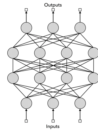
2.2.1 Feed-Forward Neural Network

Figure 2.1: Feed-Forward Neural Network

(20)

straightforward Deep Learning architectures. As presented by figure 2.1, FNN is comprised of multiple nodes organized into sequential layers such that each layer is fully connected to the next layer; as the name signify, the information in FNN only move in forward direction

from one layer to the next; it never flows back to any of the previous layers. Generally, the computation of FNN was done case follow:

• Letxn denotes the value of n-th user input.

• Letyn denotes the value of n-th output.

• Letli

n denotes the value of n-th node in i-th layer.

• Let wi_n,m denotes the weight of the connection from m-th node in (i-1)-th layer to n-th node in i-th layer.

• Letσ denotes the activation function.1

• Letbi denotes the bias that would shift the activation function.

At the input layer (or the 0-th layer), the value of the each of its node is calculated as shown below by the equation 2.3.

l_n0 =xn (2.3)

At the i-th hidden layer, the value of each of its node is calculated as shown by equations 2.4

and 2.5.

ai_n =X

m

wi_n,m·li_m−1+bi−1 (2.4)

1_{Commonly, either a Sigmoid function or a Rectified Linear Unit (ReLU) is selected to be the activation}

(21)

li_n=σ(ai_n) (2.5) At the output layer (or the I-th layer), the value of output is as shown in the equation 2.6; if FNN is used for a classification task, then the output must also be normalized by softmax

function, as shown by equation 2.7.

yn =lIn= X m w_n,mI ·l_mI−1 (2.6) Sof tmax(yn) = exp(yn) P mexp(ym) (2.7)

Like any other neural network model, before FNN is ready to be effectively used for a prediction or classification task, it has to be trained. During the training step, the neural network would fine-tune its weights based on some training samples. The process of adjusting

the weights is done using the error back-propagation technique:

• Lety denotes the output predicted by the neural network at the current state.

• Letγ denotes the target output that the neural network is expected to predict.

• Let E(y, γ) represents the loss function, which measures how far or close the predicted output y is from expected outputγ.

• Letα denotes the user set parameter known as the learning rate.

The weights are regularly updated after each set of training samples have been read.

Mathe-matically, the process of updating the weight is done as shown by equations 2.8 and 2.9:

∂E ∂wi n,m = ∂E ∂σ ∂σ ∂ai n ∂ai n ∂wi n,m = ∂E ∂σ ∂σ ∂ai n l_mi−1 (2.8) w_n,mi :=w_n,mi −α ∂E ∂wi n,m (2.9)

(22)

2.2.2 Recurrent Neural Network

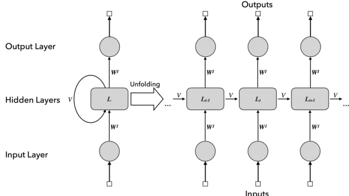
Figure 2.2: Recurrent Neural Network

Even though the modelling capability of FNN is already at an outstanding level, the

standard FNN does suffer from several major drawbacks; specifically the inabilities to model a data set with variable input size, as well as capturing the dependency of data sample to the previously seen sample. One approach address to this issue is by relegating it to the encoder

with the capability, such as the FOFE encoder.2 Another approach is to add a recurrent connection to the neural network’s structure as shown in figure 2.2. The recurrent connection allows the information to persist within the network to be used by the follow-up inputs. This

type of neural network architecture is appropriately named the recurrent neural network

(23)

(RNN).

As illustrated in figure 2.2, unfolding the RNN reveals a chain-like structure where the output of the hidden layer at the current time step is affected by the output of the hidden

layer in the preceding time step. Mathematically, the computations of RNN’s hidden layer are as following:

Li_t =σ(Vi·Li_t₋₁+Wi·Li_t−1+bi−1) (2.10) where

• VectorLi_t represents the values of all nodes in the i-th layer at the t time step.

• MatrixWi _{represents the weights of the forward connection from the (i-1)-th layer to}

the i-th layer.

• Matrix Vi represents the weights of the recurrent connection from the i-th layer at the previous time step to the i-th layer at the current time step.

• σ denotes the activation function.

• bi denotes the bias that would shift the activation function.

During the training step, RNN would update its weights using the technique known as back-propagation through time (BPTT) [11]. As the name would imply, this technique would

first unfolds the network through time, then updates the weights of unfolded RNN in the same way that back-propagation does for FNN [8].

(24)

2.2.3 Long Short-Term Memory

Even though the RNN can capture the dependency across input samples, this ability is limited to short-term dependency where the past sample that would serve as the context is not too far apart from the current input sample. In the case of long-term dependency,

the past sample context eventually become too far from the current input that its weight diminished into irrelevancy. To overcome this limitation, another variation of RNN known as the Long Short-Term Memory (LSTM) network was developed.

Figure 2.3: Long Short-Term Memory Network [12]

In LSTM, the information flows are controlled by the gate mechanism and the cell state. This enables LSTM to freely add or remove information from the cell state; simply put, the

LSTM has the ability to selectively remember or forget any information [12, 13]. Hence allows the important information to be preserved within the network for a long period; conversely, the information that deemed unnecessary could also be quickly forgotten. As shown in figure

(25)

Figure 2.4: LSTM’s Cell [12]

with a modification of using LSTM’s cell as a hidden layer. As presented by the figure 2.4 of LSTM’s cell, the information in each cell state (Ct) is depending on [13]:

• The previous cell state (Ct−1), which represents the information stored in the memory

from the previous time step.

• The previous hidden state (ht−1), which represents the output of the previous cell. • The current input (xt), which represents the new information given to the network.

(26)

As previously stated, LSTM uses gate mechanisms to manipulate the information within the LSTM’s cell. There are three main gate mechanisms in LSTM, the Forget Gate, the Input Gate, and the Output Gate.

The Forget Gate, which is responsible for dismissing the information that has lost its relevant from the cell state [13]. Mathematically, this gate is computed as follow [12]:

ft=σ(Wf ·[ht−1, xt] +bf) (2.11)

where

• ht−1 is one of the gate’s input; it is denoting previous cell’s hidden state. • xt is one of the gate’s input; it is denoting the input at current time step.

• Wf denotes the weight matrix.

• bf denotes the bias.

• σdenotes the activation function; (in standard LSTM, this would be a Sigmoid function).

• ftis the gate’s output, which ranged from 0 to 1; when ft = 0, it represent the complete

removal of this information; when ft = 1, it represent the complete preservation of this

information.

The Input Gate, which is responsible for admitting any information into the cell state [13]. Mathematically, this gate is computed as follow [12]:

(27)

ˆ

Ct =tanh(WC ·[ht−1, xt] +bC) (2.13)

where

• ht−1 is one of the gate’s input; it is denoting previous cell’s hidden state. • xt is one of the gate’s input; it is denoting the input at current time step.

• Wi and WC denote the weight matrices.

• bi and bC denote the biases.

• tanh denotes the tanh function.

• it* ˆCt is the gate’s output.

The Output Gate, which is responsible for picking out the useful information and output it. Mathematically, this gate is computed as follow [12]:

ht=σ(Wo·[ht−1, xt] +bo)∗tanh(Ct) (2.14)

where

• ht−1 is one of the gate’s inputs; it is denoting the previous cell’s hidden state. • xt is one of the gate’s inputs; it is denoting the input at the current time step.

• Ct is one of the gate’s inputs; it is denoting the current cell state.

(28)

• bo denotes the biases.

• tanh denotes the tanh function.

• ht is the gate’s output; it is denoting the current cell’s hidden state.

2.2.4 Convolutional Neural Network

Figure 2.5: Convolutional Neural Network [14]

Convolutional Neural Network (CNN) is a Deep Learning architecture that is most commonly used in image-related tasks such as image recognition, image classification, and

object detection. As illustrated in figure 2.5, CNN is primarily made-up of input layer, convolutional layers, pooling layers, fully connected layers, and output layer; the normalization

layer would also be included if CNN is being utilized in a classification task [14]. At a fundamental level, the only real difference between CNN and FNN is the addition of

(29)

convolutional and pooling layers, which are responsible for reducing the dimension of the input image while learning to preserve the features critical to the prediction.

Figure 2.6: Convolution [15]

Convolutional layer: In this layer, the input image matrix would first go through a convolution operation, which involves multiplying a section of image matrix with a filter matrix, known as Kernel, as shown in figure 2.6 [14]. As presented in figure 2.7, the Kernel would repeatedly stride over and multiply with the next section of image matrix until all

(30)

was applied to it.3

Figure 2.7: Convolution striding of 2 pixels [16]

Figure 2.8: Max-Pooling [14]

Pooling layer: When images are too large, the down-sampling process is required to reduce the number of parameters [16]. This down-sampling process in CNN is commonly

known as pooling. While there are many types of pooling methods (such as max pooling, average pooling, and sum pooling), max pooling is generally the preferred method; this is

(31)

because, in addition to down-sampling, max-pooling is also suppressing the noise [17]. The process of max-pooling is relatively simple; the machine simply has to partition the input matrix and select the highest value from each partition as shown in figure 2.8.

2.3 Deep Learning for NLP

As mentioned earlier, the Natural Language Processing (NLP) tasks are among the most

challenging for a computer system to handle; for many years, it was considered to be the Holy Grail of Artificial Intelligence (AI). However, with the recent rapid development in Deep Learning methods, Deep Learning’s neural networks have shown to be extremely suitable

for NLP; the majority of state-of-art NLP’s models are using some sort of neural networks architecture. Even the Deep Learning’s feed-forward neural network is famously known to be a powerful universal approximator that could learn to map any input units to any NLP

target [18]. In this section, we will introduce a few notable cases where deep learning’s neural network has been successfully applied to NLP tasks.

2.3.1 Deep Learning for Language Modelling

Recall that the goal of language modelling is to learn the probability distribution over a sequence of words; simply put, the language model has to learn to predict the probability

of a word appears in any specific location from given the sequence of preceding words. The language model that is a neural network is fittingly known as the Neural Network Language Model (NN-LM); in recent year, the vast majority of state-of-art language model is a NN-LM

(32)

trained through Deep Learning. Recall that the goal of language modelling is to learn the probability distribution over a sequence of words

The general idea behind NN-LM is to project the discrete words onto a continuous space,

then learn to estimate the conditional probabilities of each known word within the projected space. This task of predicting the conditional probabilities of words in the language model can be viewed as a multinomial classification problem where each word in the vocabulary is a

single class. Often in the multinomial classifier, the output score computed by the neural network has to be normalized into a probability via the softmax function. Unfortunately, the softmax computation is unbearably intensive when being applies to the extremely large output

layer. This caused the training of NN-LMs to often be incredibly slow. The solution currently used by many NN-LMs (including our models in chapter 4.3.1) is to use noise contrastive estimation (NCE) [19]. The basic idea of NCE is to reduce the probability estimation problem

into a probabilistic binary classification problem [20, 21].

2.3.2 Deep Learning for Machine Reading Comprehension

As explained previously in subsection 2.1.2, the reading comprehension task is inherently more challenging for a machine. Currently, Deep Learning has emerged to be the most successful approach for a machine to reading natural language text and extract relevant information

from it.

For simplicity, let us consider that the reading comprehension’s inputs consist of the passage, the question, and the candidate answer; let us assume that the correct target answer

(33)

must be a text segment within the passage; hence the set of candidate answers would contain every possible text segment within the passage. The machine reading comprehension (MRC) task can be treated as a binary classification problem where the MRC neural network would

determine whether the candidate answer input is the correct answer for the corresponding question and passage inputs [22]. Regarding the neural network, let us consider the LSTM network.4 _{Each word within the passage, the question, and the candidate answer was}

sequentially fed into the LSTM model. As the LSTM model takes in each word, it would generate a hidden state and a cell state, which would be passed on the next time step for reading the next word [22]. While it is possible to feed each word into the neural network

model directly in text form, it was not typically done, since it was easier for the model to process the word vector representation. Generally, a pre-trained word vector is used to initialize the word embedding matrix; this was done to preserve the contextual similarity

between words within the word vector representation. Another mechanism that is often used to improve the MRC neural network’s performance is the attention mechanism. While

there are many ways to implement the attention layer, the general idea behind them is that this layer is responsible for determining which portions of the input text containing relevant information [22]; thus allow the MRC model to place more weight on those portions of input.

4_{The LSTM was selected over other neural networks because, as we discussed in section 2.2, it could take}

in variable-sized inputs of the MRC task. While standard RNN could also take variable-sized inputs, LSTM is generally considered a superior network, since LSTM could freely remember or forget any information.

(34)

2.3.3 Deep Learning for Named Entity Recognition

Since Named Entity Recognition (NER) was not one of the tasks we were experimenting on in this thesis, it was only briefly mentioned in section 2.1; thus let us first introduce it. As the name would suggest, NER is a task of locating and classifying the named entities with

the given sequence of text. In NER, the term named entity is not only referring to a named object and concept but also numerical expressions (such as time, money, length, weight, etc). The named entity’s types are a predefined classes; it typically includes, but not limited to,

person (PER), nominal person (NPER), organization (ORG), location (LOC), facility (FAC), product (PROD), event (EVENT), time (TIME), quantity (QUAN), and none (NONE).5 _As

an example, table 2.2 shows several sentences with the named entities and their type tagged.

The NER task could be seen as a sequential classification problem where the NER system would sequentially predict the conditional probability of each possible text segment being in each of the classes, given the surrounding sequence of text as a context; the text segment

would be assigned the class with the highest probability.

Sentences

[J im]P ER and his [f amily]N P ER are moving to [Ottawa]LOC in [N ovember]T IM E.

[J ames]P ER spent total of [3grand]QU AN attending the [EM N LP]EV EN T [2019]T IM E.

[J ohn] is a transfer student from [U niversity of [Ottawa]LOC]ORG.

Table 2.2: Example sentences with named entities tagged

Classically, the NER task is typically handled by a rule-based approach. In rule-based

(35)

NER systems, the rules for determining the named entity are manually designed basing on the domain-specific gazetteer and the syntactic-lexical pattern [23]. However, the performance of rule-based NER systems depends largely on the completeness of the lexicon available; it

could not detect any hidden rule. Furthermore, the system obviously cannot be transferred to another domain outside the one it is designed for [23].

Another traditional approach to the NER task is the feature-based machine learning

approach. The feature-based machine learning approach consists of two major part:

• The hand-crafted features; this could be a word-level features (such as the case, the morphology, and the part-of-speech tag), a list lookup features (like a gazetteer), or a

document features (such as local syntax and term frequency tag) [23].

• The machine learning models such as Hidden Markov Models (HMM), Decision Trees, Maximum Entropy Models, Support Vector Machines (SVM), and Conditional Random Fields (CRF) [23].

Currently, the dominant machine learning models for the NLP task is the deep learning’s

neural network; virtually all of the recent state-of-art NER systems are utilizing this. In addition to the statistically superior classification accuracy, the deep learning based systems could be another domain outside without requiring an intensive alteration. Furthermore,

the system also can automatically discover the hidden features [23]. Noted that although the hand-crafted features are not necessary for the NER system to function as a whole,

their inclusion would often considerably improve the NER accuracy; especially the gazetteer feature, its inclusion has shown to introduce a very useful external information to the NER

(36)

system [24].

2.4 Pre-training in Deep Learning

One of the most common issues in any application of Deep Learning is the shortage of

training data; the performance of Deep Learning’s model on any specific task is intrinsically tied with the quantity and quality of the available data set. This is especially true in a diversified field like Natural Language Processing (NLP), which has many distinct tasks; in

NLP, there are hardly any task-specific data set with more than a couple of hundred thousand human-labelled training samples [25].6 _{One very successful approach to help alleviate the}

shortage of training data is known as the Pre-training.

The basic idea behind the Pre-training approach is to use a massive amount of unannotated text data (from a corpora such as the BookCorpus and Wikipedia) to train a general-purpose language representation model [25]. The pre-trained language representation could then

be applied to a downstream NLP task (like named entity recognition, machine reading comprehension, sentiment analysis, etc); there are two main approaches in which this step could be performed:

• Thefeature-basedapproach where the pre-trained representations are used as additional features for the downstream task’s architecture [26].

• Thefine-tuningapproach where the pre-trained model is being further train by fine-tune

6_{While a couple of hundred thousand samples in a data set may appear large at a glance, a Deep Learning’s}

(37)

all of the pre-trained parameters on the downstream NLP task’s data set [26].

For the next part of this section, we will provide a brief literature review on one of the well-known pre-trained language representation called the Bidirectional Encoder Representations

from Transformers (BERT). This language representation is of interest to us, because the SQuAD1.1 corpus, which we have experimented on, has the vast majority of its top-scoring models (including the state-of-art model) utilize some variant of BERT.

2.4.1 Bidirectional Encoder Representations from Transformers

(BERT)

BERT is a deep bidirectional language representation that was designed to be pre-train on an unlabeled text corpus [25]. The overall procedure of training BERT model has two main

steps, the pre-training step and thefine-tuning step [26].

• During the pre-training step, the BERT model is being pre-trained on the unlabeled text corpus with the “masked language model” (MLM) task and the “next sentence

prediction” task as its pre-training objectives [26]. The BERT models presented by Devlin et. al. in their paper [26] were trained on the BooksCorpus and the Wikipedia. Noted that the task of MLM is to predict the identity of a randomly masked word

within the input text. Since MLM utilizes both the left and the right context for its prediction, the BERT model could be pre-train as a deep bidirectional Transformer [26].

(38)

with the value from the pre-trained general-purpose model, all pre-trained parameters are then fine-tuned using the downstream NLP task’s data set [26]. Noted that through fine-tuning, different downstream NLP tasks would ultimately end up with different

BERT models [26].

The distinguishing quality of BERT is that it has a general methodology that could be applied for practically all NLP tasks; as illustrated by figure 2.9, there is hardly any difference between

the BERT’s pre-trained architecture and the BERT’s fine-tuned architecture (regardless of which down-stream task it being fine-tuned for) [26].

(39)

Chapter 3 Fixed-size Ordinally-Forgetting

Encoding (FOFE)

For a Deep Learning model to effectively process any natural language, the natural language

inputs (such as characters, words, or sentences) have to first be encoded into a vector representation. Depending on the encoder being use, the vector representation could offer

several benefits. For instance, an equivalently defined sentence could be encoded to have close vector values. Another example, the encoder could also assign the vector values based on the frequency of the words being used. In this chapter, we will be reviewing the

Fixed-size ordinally-forgetting encoding (FOFE) method and the FOFE based neural network (FOFE-net).

(40)

3.1 Related Encoding Methods

Before we introduce FOFE and FOFE-net, let us first go over several other related encoding methods, namely the One-Hot Encoding and the Bag-of-Words.

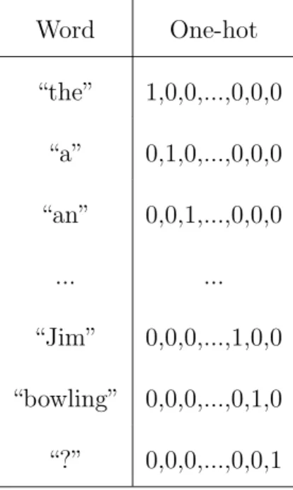
3.1.1 One-Hot Encoding

One-hot encoding is a word-level encoding method, where all the words within the vocabulary (that is given to the machine) are assigned a fixed vector representation called a one-hot

vector. In the one-hot vector, one member must have a value of 1, while the rest must have the values of 0. Word One-hot “the” 1,0,0,...,0,0,0 “a” 0,1,0,...,0,0,0 “an” 0,0,1,...,0,0,0 ... ... “Jim” 0,0,0,...,1,0,0 “bowling” 0,0,0,...,0,1,0 “?” 0,0,0,...,0,0,1

Table 3.1: Examples of One-Hot Encoding

One of the major weaknesses of one-hot encoding is that it treats each word as an independent input; thus semantic similarity between word is lost when converted to one-hot

(41)

representation [8].

3.1.2 Bag-of-Words

Bag-of-Words (BoW) is one of the simplest sentence-level encoding method. A sentence (or a word sequence) is represented by a summation of the one-hot vector of each word making up the sequence. The main deficiency of BoW representation is that it ignores the order of each

word in the sequence. Hence the multiple sentences with vastly different meanings could end up with the same BoW representation [8]; as an example of such case, consider these two sentences, “Person A is older than person B” and “Person B is older than person A”.

3.2 FOFE

Fixed-size ordinally-forgetting encoding (FOFE) is an encoding method that generates a fixed-size representation, namely the FOFE code, for any variable-length word sequence [1].

Furthermore, the FOFE encoding is also said to be a unique and lossless encoding, meaning that any FOFE code could be transformed back into the original word sequence [1]. In this

section, we will provide the formal definition of FOFE, the intuition behind the concept, as well as the formal proof of the FOFE code’s uniqueness.

3.2.1 Definition of FOFE

For a given word sequence S = {w1, w2, ..., wT}, let et denotes the one-hot representation of

(42)

Word One-hot w0 1,0,0,0,0,0,0 w1 0,1,0,0,0,0,0 w2 0,0,1,0,0,0,0 w3 0,0,0,1,0,0,0 w4 0,0,0,0,1,0,0 w5 0,0,0,0,0,1,0 w6 0,0,0,0,0,0,1

Table 3.2: Vocabulary of size 7

Word Sequences FOFE Code

w5 0, 0, 0, 0, 0, 1, 0

w5, w4 0, 0, 0, 0, 1,α, 0 w5, w4, w2 0, 0, 1, 0, α, α2, 0 w5, w4, w2, w4 0, 0, α, 0, α2+1, α3, 0 w5, w4, w2, w4, w0 1, 0, α2, 0, α3+α, α4

(43)

as follows:

zt=α·zt−1 +et (1≤t≤T) (3.1)

where α (0 < α <1) denotes the forgetting factor, a parameter responsible for determining the degree of influence each time step of the past context has on the FOFE code. Obviously, FOFE can convert any variable-length sequence into a fixed-size code with length equal to the size of vocabulary. As an example, we provided the tables 3.2 and 3.3 to show the FOFE

encoding of word sequence {w5, w4, w2, w4, w0}.

3.2.2 Intuition behind FOFE

From a certain perspective, FOFE could be considered an improved version of BoW encoding

with the addition of forgetting factor; the inclusion of a forgetting factor allows the encoding to capture positional information of the word sequence, hence effectively resolved the BoW’s main deficiency concerning the potential to produce the same encoding from different word

sequences [8].

3.2.3 Uniqueness of FOFE Code

Regarding uniqueness of FOFE code, the FOFE is said to be unique and lossless encoding

under these two theorems [27]:

Theorem 1 If 0 < α≤ 0.5, then FOFE code is guarantee to be unique for any finite values of vocabulary’s size and sequence’s length.

(44)

code zT ={c1, c2, ..., cK}where K denotes vocabulary’s size and T denotes sequence’s length.

Let wi _{denotes the i-th word in vocabulary. If}_c

i has a value of αt, then the word wi must be

in the position t of sequence S, since whenα ≤ 0.5 [27]:

• Even ifwi showed up every positions before t (and no where else), it still would not sum up to αt_.

• Conversely ifwi _{showed even up once in position after t, the value of}_c

i must be greater

than αt.

Theorem 2 If 0.5 < α < 1, then FOFE code is guarantee to be almost unique for any finite values of vocabulary’s size and sequence’s length, except for a finite set of countable choices of α.

Proof: Let us consider decoding a given FOFE codezT ={c1, c2, ..., cK} in order to obtain

an unknown word sequence S = {w1, w2, ..., wT} where K denotes a vocabulary’s size and

T denotes a sequence’s length. Let wi denotes the i-th word in vocabulary. For any ci =

1.0 when 0.5 < α < 1, there are two possible cases that could lead to an ambiguity in the decoding of this FOFE code [27]:

• The wordwi appears once in the last position of sequence S.

• The word wi _{appears multiple times within sequence S and their total contribution}

happens to sum up to 1.0.

(45)

polynomial equations:

T X

t=1

ξt·αt= 1.0 (3.2)

where ξt = 1 if the word wi appears in the position t (1≤t≤T) of sequence S, otherwise ξt =

0. Since each polynomial equation in 3.2 is of T-th order, there can be at most T real roots

for α [27]. Furthermore due to ξt = {0,1}, the total number of equation in the form of 3.2

can be no more than 2T _{[27]. Hence there can be at most} _T _·₂T _{choice of} _α _{that could cause}

an ambiguity in decoding [27].

Figure 3.1: Result for FOFE codes’ collisions simulation [27]

However, the chance of actually having any collisions for α between 0.5 and 1 is nearly impossible in practice, due to quantization errors in real computer systems. To prove this,

(46)

Zhang et. al. have conducted an experimental simulation counting the number of collisions for all possible sequences up to 20 symbols [27]. Noted that a collision is only counted if the highest element-wise difference between two FOFE codes is less than the epsilon threshold [27].

Base on the result shown in figure 3.1, the number of collisions encountered is extremely low. Hence in practice, it is safe to argue that FOFE can uniquely encodes any variable-length sequence into a fixed-size representation.

3.3 FOFE-net

Figure 3.2: FOFE-net

As indicated by figure 3.2, the FOFE based neural network (FOFE-net) is essentially a combination of FOFE encoder and Feed-forward neural network (FNN); in FOFE-net, the

(47)

inputs would first be encoded by the FOFE encoding layer before passed on to the hidden layers and then an output layer.

As previously introduced in subsection 2.2.1, FNN is the most straightforward of all Deep

Learning’s neural network. However, FNN is still known to be a universal approximator with an extremely powerful modelling capability, which allows it to learn to map any input units to any NLP target [18]. Furthermore, the straightforwardness of FNN allows it to not be as

computationally demanding as other neural networks such as CNN, RNN, and LSTM; this ultimately results in FNN also being faster to train. This factor is particularly beneficial for the field of NLP since many of the tasks required the neural network to learn from a

large data set. Despite all these benefits, FNN is generally not as favoured as the other Deep Learning’s neural network, due to its two main limitations; specifically its inabilities to model a data set with variable input size, as well as to capture the dependency across samples in

the data set.

However these limitations do not apply to FOFE-net since FOFE could uniquely encode

any variable-length input sequence into the fix-sized FOFE code; furthermore, since the value of FOFE code was influenced by the value of past inputs, the FOFE code could also said to have captured the dependency across input samples.

(48)

Figure 3.3: 1st-order FOFE FNN-LM

3.4 Higher-Order FOFE

As illustrated by figure 3.3 7_{, the FOFE code could be efficiently computed via a time-delayed}

recursive structure, where the symbol z−1 _{in the figure represents a unit time delay (or}

equivalently a memory unit) from zt to zt−1. With this time-delayed recursive structure,

FOFE could easily be scaled up to order as shown in figures 3.4 and 3.5; the

higher-7_{Noted that the projection step could be implemented before or after the FOFE step since both steps are}

(49)

order FOFE allows the previous FOFE encoded input to be utilized as an additional context without any substantial increase in computational complexity.

(50)

(51)

Chapter 4 Dual Fixed-size Ordinally-Forgetting

Encoding (Dual-FOFE)

As indicated in chapter 3, the key parameter of the FOFE method is known as the forgetting

factor; this parameter is responsible for determining the degree of sensitivity of the encoding with respect to the past context. In the original FOFE method, selecting a good value for

the single forgetting factor could be tricky since both small and large forgetting factors are offering different benefits; specifically it is the issue of balancing between FOFE’s abilities to capture the positional information and to model long-term dependency. To resolve this

trade-off issue, we propose an alteration to the FOFE method, which allows us to incorporate two forgetting factors into the fixed-size encoding of the variable-length word sequences. We name this approach as dual-FOFE. We hypothesize that by incorporating both the small and

(52)

optimize the abilities to capture the positional information as well as to model long-term dependency.

The main idea of dual-FOFE is to generate augmented FOFE encoding codes by

con-catenating two FOFE codes using two different forgetting factors. Each of these FOFE codes is still computed in the same way as the mathematical formulation shown in Equation (3.1). The difference between them is that we may select to use two different values for the

forgetting factor (denoted asα) for additional modelling benefits.

4.1 Intuition behind Dual-FOFE

As mentioned in the chapter 3, the values in a FOFE code are used to encode both the content and the order information in a sequence. This is achieved by a recursive encoding method where at each recursive step the code will be multiplied by the forgetting factor (α) whose value is bounded by 0 < α <1. In a practical computer with finite precision, this has an impact on the FOFE’s abilities to precisely memorize the long-term dependency of past context as well as to properly represent the positional information.

The FOFE’s ability to represent the positional information would improve with a smaller forgetting factor. The reason is that that when α is small, the FOFE code (zt) for each word

vastly differs from its neighbour in magnitude. If α is too large (close to 1), the contribution of a word may not change too much no matter where it is. This may hamper the following neural networks to model the positional information. Conversely, the FOFE’s ability to model the long-term dependency of the older context would improve with a larger forgetting

(53)

factor. This is because whenαis small, the contribution of a word from the older history may quickly underflow to become irrelevant (i.e. forgotten) when computing the current word.

In the original FOFE with just a single forgetting factor, we would have to determine the

best trade-off between these two benefits. On the other hand, the dual-FOFE does not face such issues since it is composed of two FOFE codes: the half of the dual-FOFE code using a smaller forgetting factor is solely optimized and responsible for representing the positional

information of all words in the sequence; meanwhile, the other half of the dual-FOFE code using a larger forgetting factor is optimized and responsible for maintaining the long-term dependency of past context.

4.2 Dual-FOFE vs. Higher-Order FOFE

As noted previously in the section 3.4, the higher-order FOFE codes would utilize both the

current and the previous sequence FOFE codes for prediction. Hence similar to dual-FOFE, the higher-order FOFE could also maintain the sensitivity to both nearby and faraway contexts. Obviously, a much higher-order FOFE code may be required to achieve the same

effect as dual-FOFE in terms of modelling long-term dependency. In this case, the higher-order FOFE may also significantly increase the number of parameters in the input layer. At last, the dual-FOFE and the higher-order FOFE are largely complementary since we have

observed consistent performance gains when combining dual-FOFE with either 2nd-order or 3rd-order FOFE in our experiments.

(54)

4.3 Dual-FOFE-net’s Applications

Much like FOFE-net, the Dual-FOFE based neural network (Dual-FOFE-net) could be applied to almost all NLP tasks, so long as their enough training data. This is because the

Dual-FOFE-net is made up of:

• The Dual-FOFE encoder, a lossless invertible encoder that could encode any variable-length input into a fixed-size representation.

• The FNN, a universal approximator that could learn to map a fixed-size input to any NLP target.

To demonstrate the effectiveness of Dual-FOFE, we have performed experiments on two prominent NLP tasks, the language modelling and the machine reading comprehension.8 _In

this section, we will be providing an overview of our application of Dual-FOFE-net on these two tasks.

4.3.1 Dual-FOFE for Neural Language Model

Figure 4.1: Example of Dual-FOFE usage in Language Modelling

(55)

The idea of dual-FOFE based Neural Network Language Models (NN-LMs) is to use dual-FOFE to encode the partial history sequence of past words in a sentence, then feed this fixed-size dual-FOFE code to a feed-forward neural network as an input to predict next word.

For example, given a sentence S = {w1, w2, ..., wT}, where each word wt is represented by a

one-hot vector et. A set of input samples ({z1, z2, ..., zT} for feed-forward neural network can

be extracted from sentence S; each input samplezt is a FOFE encoding of partial sentence

{w1, , ..., wt−1, wt} up to word wt.

(56)

Figure 4.3: 3rd-order Dual-FOFE FNN-LM

The three figures (3.3, 3.4, and 3.5) presented on section 3.4 are the illustrations of

original FOFE based NN-LMs used by Zhang et. al. in their paper [1]. As shown in figures 4.2 and 4.3, the architecture of dual-FOFE based FNN-LMs is very similar to the original FOFE FNN-LMs. In the Dual-FOFE FNN-LMs, the input word sequence would have to

pass through two branches of the FOFE layers (using two different forgetting factors) and each encoding branch will produce a FOFE code representing the input sequence. These two FOFE codes are then joined to produce the dual-FOFE code, which would be fed to FNNs

(57)

to predict the next word.

It might also be worth noting that in our implementation we do not explicitly reset FOFE codes, i.e. zt value, at sentence boundaries. However, far-away histories will be gradually

forgotten by the recursive calculation in FOFE due to 0 < α < 1 and finite precision in computers.

The Order of Projection Layer and FOFE Layer are Interchangeable

Noted that the FOFE FNN-LM’s figures presented in Zhang’s original FOFE paper [1] are

slightly different from our FOFE FNN-LM’s figures ( 3.3, 3.4, and 3.5) and Dual-FOFE FNN-LM’s figures (4.2 and 4.3); the order of our projection layer and FOFE Layer have switched. The difference in the location of our layers is simply indicated two equivalent

ways to do word projection in conjunction with word sequence encoding. Both methods are mathematically equivalent since both projection and FOFE steps are linear. Although it is

more efficient to do projection as in figures 4.2 and 4.3, hence we chose to implement our architecture this way instead.

• Let us consider an input word sequence S = {w1, w2, ..., wT}.

• Letet (1≤et ≤T) be a one-hot vector representing word wt.

• Let T denote the length of sequence S.

• Let K denote the vocabulary’s size.

(58)

• Let X = [e1, e2, ..., eT] denote a T ×K matrix representing one-hot encoding of each

word in sequence S row-by-row.

• Let U = [u1, u2, ..., uK] denote a K ×D word embedding matrix where D denotes a

word embedding dimensions; in our case, we are using GloVe word embedding with 300

dimensions.

• ThereforeF OF E(α, X)·U = (A·X)·U represent a computation of FOFE layer follow by projection layer.

• Meanwhile F OF E(α, X·U) =A·(X·U) represent a computation of projection layer follow by FOFE layer.

(A·X)·U =                 1 α 1 α2 α 1 .. . ... . .. 1 αT−1 _αT−2 _{. . .} _α ₁                 ·                 e1 e2 e3 .. . eT                 ·                 u1 u2 u3 .. . uK                 =A·(X·U) (4.1)

4.3.2 Dual-FOFE for Machine Reading Comprehension

The architecture of our dual-FOFE based FNN for Machine Reading Comprehension

(Dual-FOFE FNN-MRC) is composed of 5 main components: the pre-processor, the encoder, the

sampler, the neural network, and the decoder; as shown in figures 4.4 and 4.5, the decoder and the sampler are exclusively used during testing phase and training phase, respectively. The figures 4.6 and 4.7 are illustrating the high-level overview of Dual-FOFE FNN-MRC’s

(59)

Figure 4.4: Dual-FOFE FNN-MRC (in Testing Phase)

architecture; as outlined by these diagrams, the reading comprehension’s inputs are processed

by the aforementioned main components in sequential order.9 In the next part of this section, we will provide a more in-depth overview of these 5 components.

The Pre-processor: The raw input question and passage have to first be preprocessed into input features before our model can properly utilize them; during this process, the

9_{Noted that the loss function was not listed among the main components despite being present in figure}

(60)

(61)

(62)

(63)

important information is extracted and transformed into a desired format. The resultant input features include:

• The question that our model is predicting the answer for.

• The candidate answers, which are the set of texts where each of the members is a candidate for being the correct answer. During the testing phase of our model, the candidate answers would consist of every possible text segment taken from the passage. However, during the training phase of our model, a portion of the incorrect candidate

answers will be filtered out by the sampler in later steps.

• Theleft-contexts, which is referring to the words in document passage that are within the same sentences and to the left of the corresponding candidate answer. The left-contexts could either include or exclude the candidate answer from its sequence; in this case, we chose to keep both versions as it improves our model’s prediction accuracy.

• Theright-contexts, which is referring to the words in document passage that are within the same sentences and to the right of the corresponding candidate answer. The

right-contexts could either include or exclude the candidate answer from its sequence; similar to the left-contexts, we also chose to keep both versions of right-contexts.

• Thequestion-passage matching tag, an optional input feature that tags all words in the passage that also exist in the question.

• The passage’s term frequency (TF), an optional input feature which recorded the term frequency of each word in the passage.

(64)

• The passage’s part-of-speech (POS) tag, an optional input feature that tags each word in the passage with POS grammatical tag.10

• The passage’s entity tag, an optional feature that tags all words in the passage that are an entity.11

After the input features have been extracted from raw input data, the core features (such as

the question, the candidate answers, the left-contexts and the right-contexts) that are being represented in text were then converted into word vectors; noted that by using a pre-trained word vector to initialize word embedding matrix, we are able to preserve the contextual

similarity of words.12 Regarding the 4 optional input features, they were identified as such because their inclusions are not necessary for our Dual-FOFE FNN-MRC to function; however they were included, since they provided a substantial improvement to our model’s prediction

accuracy.

Figure 4.8: High-Level Diagram of Pre-processor

10_{This grammatical tagging was done with the aid of spaCy’s POS tagger.}

11_{This entity tagging was done with the aid of spaCy’s named entity recognizer (NER).}

12_{The pre-trained word vector that we are used for our MRC is the word vector released by Stanford}

(65)

(66)

The Encoder: Following the preprocessing step, the resultant input features are then passed on to the encoder. As indicated by the name of our model, the encoder we are using is dual-FOFE; since our FNN-MRC model is using feed-forward neural network, the encoder

that could produce a fixed-size vector (from any variable-size sequence), as well as guaranteed theoretical uniqueness like dual-FOFE encoder, is ideal. For this subsection, we will be using three variations of dual-FOFE encoders specifically chosen for each input feature that is being

employed here. The three variations of dual-FOFE encoders are:

• The Forward Dual-FOFE encoder is being deployed for the left-context input feature. This is a regular dual-FOFE encoder where the two FOFE encoders (within dual-FOFE)

would encode the input sequence in the rightward order. Hence the right side of the left-context sequence, which is closer to the candidate answer, would have higher weight. Conversely, the further left along the left-context sequence (away from candidate

answer), the smaller the weight became; the weight could ultimately underflow to 0, signifying that this section of context sequence is too far away from candidate answer to be of any relevance.

• TheBackward Dual-FOFE encoderis being deployed for the right-context input feature. This is a reversed FOFE encoder where the two FOFE encoders (within dual-FOFE) would encode the input sequence in the leftward order. Hence the left side

of the right-context sequence, which is closer to the candidate answer, would have higher weight. Conversely the further right along the right-context sequence (away from candidate answer), the smaller the weight became and would underflow to 0 for

(67)

the sequence that has exceeded a certain length.

• TheBidirectional Dual-FOFE encoderis being deployed for the questions, the candidate answers, the question-passage matching tag, the passage’s TF, the passage’s POS

tag, and the passage’s entity tag input features. As its name would suggest, this is a concatenation of Forward Dual-FOFE and Backward Dual-FOFE; hence allowed the encoder to place equal importance to both left and right sides of the input sequence.

(68)

(69)

The Sampler: During the training phase, the next process following the encoding step is the sampling step; meanwhile during the testing phase, the model will be skipping this step. As mentioned earlier, the candidate answers fundamentally have included every possible text

segment taken from the passage. However only one of these text segments can potentially be the correct answer. Hence the ratio of correct sample to incorrect samples was heavily skewed, which was detrimental to the training process of our neural network as it caused the

model to become bias toward classifying any candidate as being incorrect. To prevent this, the single correct candidate answer and a random portion of the incorrect candidate answers are selected as a sample for the training process of the neural network model. Based on our

experiment, the best sampling ratio for our sampler is selecting:

• 1 positive sample where a positive sample is referring to the sample whose candidate answer is the correct answer.

• 10 partially negative sampleswhere a partially negative sample is referring to the sample whose candidate answer is incorrect but is overlapping the correct answer.13

• 140 completely negative samples where a completely negative sample is referring to the sample whose candidate answer is incorrect and is not overlapping the correct answer.

13_{Noted that during the training of the neural network, the partially negative samples are treated as a}

(70)

Figure 4.11: Examples of Sampler’s Inputs & Outputs

The Neural Network: The neural network chosen for this experiment is the feed-forward neural network (FNN). As a universal approximator, FNN could learn to map

any input units to any NLP target including that of reading comprehension [18]. While FNN is a powerful computation model, its usage is often restricted by its inability to take variable-length input and to capture long-term dependency. However, this is not an issue for

our Dual-FOFE FNN, since dual-FOFE (as well as FOFE) can produce a fixed-size encoding from any variable-length input as well as to model the long-term dependency.14

As presented in figures 4.4 and 4.5, the FNN would take in the dual-FOFE encoded input

features (including the question, the candidate answers, the left-context, the right-context, and the four optional features) as its input, then output the score signifying the likelihood of

(71)

the corresponding candidate being the correct answer. In the testing phase, this step would end here, the score for all the candidate answers would be collected and passed onto the decoder. Alternatively in the training phase, our model would then use the cross-entropy loss

function on the FNN’s assigned score and the expected score to compute the loss value that measures how close (or far) the FNN’s score is in comparison to the expected score; afterward, the model would proceed to back-propagate through each FNN’s layer while adjusting the

weights of their nodes in order to reduce loss value for the next training sample.

Figure 4.12: Examples of Neural Network’s Inputs & Outputs

The Decoder: During the testing phase, the next process following the neural network is the decoding step. At this stage, all the possible candidate answers have been tested and assigned a score by our FNN. The decoder would then select the candidate answers whose

(72)

within the input passage; this text is our model’s predicted answer to the input question.

Figure 4.13: Examples of Decoder’s Inputs & Outputs

Dual-FOFE Encoder as Passage’s Scanner

Previously we have explained the simplistic design of Dual-FOFE MRC where the pre-processor and the encoder are entirely separate modules. However, dual-FOFE encoder could

be implemented in a way to scan for all possible candidates (and their associated left-contexts and right-contexts), while encoding them. Essentially, the dual-FOFE encoder is partially taking on the job of pre-processor; hence the new architecture for Dual-FOFE FNN-MRC’s

pre-processor and encoder is as shown in figure 4.15, opposed to the original architecture shown by figure 4.14. To achieve this, the trick is in the arrangement of the FOFE’s forgetting factor matrices.

(73)

Figure 4.14: Dual-FOFE FNN-MRC’s Pre-processor and Encoder (Original Architecture)

Figure 4.15: Dual-FOFE FNN-MRC’s Pre-processor and Encoder (Improved Architecture)

Let us consider a given word sequence S = {w1, w2, ..., wT}where each word wt could be

represented by a one-hot vector et (1 ≤et≤T). The FOFE codes for all possible candidate

answers in S, as well as their corresponding left-contexts and right-contexts, can be computed

as follow:15

• Let T denote the length of sequence S.

15_{For simplicity, we presented the forgetting factor matrices of original FOFE encoder. In dual-FOFE}

encoder, there would be two versions of forgetting factor matrices; one for smaller forgetting factor value and another for larger forgetting factor value.

(74)

• Let K denote the vocabulary’s size.

• Let A denote a T ×T FOFE’s forgetting factor matrix.

• Let X = [e1, e2, ..., eT] denote a T ×K matrix representing one-hot encoding of each

word in sequence S row-by-row.

F OF E Candidates(α, X) = Bidirectional F OF E Candidates(α, X) =Concat(F orward F OF E Candidates(α, X),

Backward F OF E Candidates(α, X))

(75)

F orward F OF E Candidates(α, X) =                                                         1 α 1 α2 _α ₁ .. . ... . .. 1 αT−1 _αT−2 _{. . .} _α ₁ 1 α 1 .. . . .. 1 αT−2 _{. . .} _α ₁ 1 α 1 α2 _α ₁ 1 α 1 1                                                         ·                 e1 e2 e3 .. . eT                 =AF C·X (4.3)

Dual Fixed-Size Ordinally Forgetting Encoding (FOFE) For Natural Language Processing

Abstract

Acknowledgements

Table of Contents

List of Tables

List of Figures

Chapter 1

Introduction

1.1

Motivation

1.2

Contribution and Thesis Organization

Chapter 2

Deep Learning for Natural Language

Processing

2.1

Natural Language Processing at glance

2.1.1

Language Modelling

2.1.2

Machine Reading Comprehension

2.2

Deep Learning Models

2.2.1

Feed-Forward Neural Network

2.2.2

Recurrent Neural Network

2.2.3

Long Short-Term Memory

2.2.4

Convolutional Neural Network

2.3

Deep Learning for NLP

2.3.1

Deep Learning for Language Modelling

2.3.2

Deep Learning for Machine Reading Comprehension

2.3.3

Deep Learning for Named Entity Recognition

2.4

Pre-training in Deep Learning

2.4.1

Bidirectional Encoder Representations from Transformers

(BERT)

Chapter 3

Fixed-size Ordinally-Forgetting

Encoding (FOFE)

3.1

Related Encoding Methods

3.1.1

One-Hot Encoding

3.1.2

Bag-of-Words

3.2

FOFE

3.2.1

Definition of FOFE

3.2.2

Intuition behind FOFE

3.2.3

Uniqueness of FOFE Code

3.3

FOFE-net

3.4

Higher-Order FOFE

Chapter 4

Dual Fixed-size Ordinally-Forgetting

Encoding (Dual-FOFE)

4.1

Intuition behind Dual-FOFE

4.2

Dual-FOFE vs. Higher-Order FOFE

4.3

Dual-FOFE-net’s Applications

4.3.1

Dual-FOFE for Neural Language Model

4.3.2

Dual-FOFE for Machine Reading Comprehension