Forecasting Stock Market Realized Volatility using decomposition

(1)

Volume 14, Issue 3 available at www.scitecresearch.com/journals/index.php/jrbem

2661

|

SCITECH

Volume 14, Issue 3

RESEARCH ORGANISATION

April 16, 2020

Journal of Research in Business, Economics and Management www.scitecresearch.com

Forecasting Stock Market Realized Volatility using

Decomposition

Rim Ammar Lamouchi

1,2,3

1

Department of Finance, Faculty of Economics and Administration, King Abdulaziz University, Saudi

Arabia, E-mail :

Ministry of Education, Tunisia.

3

GEF-2A Laboratory, Higher Institute of Management of Tunis, Tunis University, Tunisia,

Email :

Empirical studies concerned with realized volatility reveal the presence of heterogeneous behavior within the stock market. The sum of this heterogeneous behavior takes a persistent form, which may be modeled and forecasted according to different time horizons by the class of HAR models. In this paper, we investigate the HAR-RV and HAR-RV-CJ models for high-frequency data based on five realized volatility indices. The aim here is to demonstrate that the predictability of realized volatility can be improved by decomposing realized variance into its continuous and jump components. What is more, the results show that this decomposition of the realized variance into its components does indeed enhance the modeling and forecasting of the indices’ realized volatility.

Keywords: Stock market; realized volatility; high-frequency data; HAR model; variance decomposition; volatility forecasting; jumps.

Classification JEL

: C22; G15; G17.

1. Introduction

The progressive integration of the world’s financial markets has given rise to numerous studies focused on volatility in the stock market, which is something that is fairly important for hedging strategies, risk management, and the regulation of financial markets. Volatility is a complex phenomenon in a stock market. The subprime financial crisis and the subsequent sovereign debt crisis triggered a renewed interest in studying the volatility process and the existence of jumps in the stock market. Furthermore, empirical literature indicates how the market is characterized by the presence of jumps in volatility indices (Andersen et al., 2007; Busch et al., 2011). These jumps result from macroeconomic information, financial crises, or exogenous shocks. Corsi (2009) assumes that asset returns exhibit both continuous changes (diffusion) and discontinuous responses (jumps) to news. However, most empirical models ignore the jumps entirely or model them simplistically using a Poisson process and assume the presence of independent jumps. These jumps are often associated with specific announcements about macroeconomic information. The increasing availability of high-frequency data for financial markets has not only improved realized volatility measurements but also inspired research into their value as a means for forecasting volatility. In this paper, we seek to examine the existence of these jumps and assess their impact on the modeling and forecasting of realized volatility indices in the stock market.

(2)

2662

|

Previously, Barndorff-Nielsen and Shephard (2004) introduced the concept of bipower variation, which allows the jump component to be separated from the continuous part of a process. This concept in turn enables the decomposition of realized volatility into its continuous sample path and its jump components, so they can be modeled separately. Several studies have recently attempted to show the importance of jumps in financial returns, especially for realized volatility resulting from high-frequency returns. According to Andersen et al. (2003), the use of high-frequency data ensures that realized volatility converges in probability to a quadratic variation. The bipower variation is based on the sum of the absolute values of intraday returns. More precisely, Barndroff-Nielsen and Shepard (2004) show that this variation converges in probability to the continuous component of the price of the quadratic variation. Consequently, it is possible to estimate jumps in the return process as the difference between the realized volatility and the bipower variation. Andersen et al. (2007) incorporated the bipower variation measure into the HAR model and applied it to the DEM/USD exchange rate, the S&P500 market index, and the 30-year US Treasury bond yield. They demonstrated that volatility modeling and forecasting was improved by separating jumps from non-jump movements. In addition, they showed that jumps are related to announcements of macroeconomic news.

Beine et al. (2007) studied the relation between central bank intervention and the volatility of two major exchange rates. They applied the bipower variation to decompose the realized volatility into its continuous and jump components, deducing that interventions trigger considerable jumps. Fuentes et al. (2009), meanwhile, compared four estimators— namely realized volatility, realized range, realized power variation, and realized bipower variation—by investigating their in-sample distributional pattern and an out-of-sample forecast. Their analysis used a seven-year sample of prices for 14 stocks listed on the NYSE. The forecast was then generated with a GARCH framework. The authors then concluded that the combination of all four intraday measures gave the lowest forecast errors in about half the sampled stocks. Bollerslev et al. (2009) applied nonparametric realized variation and bipower variation measures constructed from high-frequency data with the aim of developing a discrete-time daily stochastic volatility model that could distinguish between the jump and continuous components of return movements. They suggested that the model allows for the consideration of structural inter-dependencies between shocks to returns and volatility components. Andersen et al. (2011) also applied a volatility decomposition method based on long samples of high-frequency data for equity and bond futures returns. Their results suggested that dynamic dependencies and variability in the continuous element can be well described by an approximate long-memory HAR-GARCH model. In addition, the dynamic dependencies in the identified significant jumps seemed to be well expressed by the ACH model with a simple log-linear structure for the jump sizes. The authors highlighted the superior forecasting performance of the model that considered both components of volatility when compared to other commonly used models. In order to take into account the impact of jumps, Barunik et al. (2016) applied a GARCH forecasting model with decomposed realized volatility measurements. They therefore decomposed volatility into several timescales, thus approximating the behavior of traders at corresponding investment horizons. They then compared forecasts by employing some current realized volatility measures for FOREX futures data for the recent financial crisis. Their results indicated that separating jump variation from the integrated variation improved forecasting performance.

The existing finance literature has extensively investigated the concept of volatility forecasting for the stock market. Most studies have focused on using ARFIMA and GARCH models (Bollerslev et al., 1994; Degiannakis, 2004; Hansen and Lunde,2005, Koopman et al., 2005; Degiannakis, 2008; Wei, 2012) to study volatility patterns. Nevertheless, one strand in the literature suggests that HAR models for realized volatility indices are more efficient at forecasting future volatility because they can capture the long-memory pattern of volatility (Corsi, 2009; Busch et al., 2011; and Fernandes et al., 2014). In this study, we aim to determine whether decomposing realized volatility into its continuous sample path and its jump components improves the modeling and forecasting of realized volatility indices for five stock indices, namely the FTSE (FTSE 100-UK), FCHI (CAC 40 100-France), GDAXI (DAX-Germany), SSMI (Swiss Stock Market Index), and FTMIB (FTS MIB-Italy).We therefore follow the example of Andersen et al. (2011) in modeling the realized volatility components separately. To model the realized volatility and its continuous component for the different exchange rates, we apply the HAR-RV model of Corsi (2009). We also compare the HAR-RV and HAR-RV-CJ models to assess whether jumps matter in the return process. To evaluate if the HAR model is suitable for realized volatility modeling, we perform a year-by-year estimation of the parameters followed by a one-year, out-of-sample forecast using pre-forecast periods of various lengths. Different stock indices are also considered to determine whether the effects differ between different stock indices.

The remainder of this paper is organized as follows: In the following section, we present our methodology for realized volatility decomposition and specify the HAR-RV models. In section 3, we discuss the data used in the study. The empirical results and forecast comparisons are then presented in section 4, with section 5 then giving the study’s conclusions.

(3)

2663

|

2. Methodology

2.1. Realized volatility decomposition

We consider realized volatility in terms of its continuous sample path and its jump components, so we introduce an element of decomposition into the daily return variance. If we consider the stock return over [t-h, t] as the difference between the logarithmic price at time t and the logarithmic price at timet-h:

𝑟𝑡,ℎ= 𝑝𝑡− 𝑝𝑡−ℎ(1)

we can then define the realized variance as:

𝑅𝑉𝑡,ℎ= 𝑟_{𝑡−ℎ +}𝑖 𝑛 ℎ

2 𝑛

𝑖=1 (2)

Where n represents the number of observations over time interval [t-h, t].

The bipower variation introduced by Barndorff-Nielsen and Shepard (2004) and later adapted by Andersen et al. (2011) is defined as: 𝐵𝑉𝑡,ℎ = 𝜇1−2 𝑛_{𝑛 −2} 𝑟_{𝑡−ℎ +(}𝑖−2 𝑛 )ℎ 𝑛 𝑖=3 𝑟_{𝑡−ℎ +(}𝑖 𝑛)ℎ (3) where𝜇1= 2/𝜋 .

We base the decomposition of 𝑅𝑉𝑡,ℎon 𝑅𝑉𝑡,ℎ− 𝐵𝑉𝑡,ℎ, but this difference can take a negative value. Consequently, to

ensure a non-negative value for the jump component, the measure proposed by Barndorff-Nielsen and Shepard (2004) can be used instead:

𝐽𝑡,ℎ= max[𝑅𝑉𝑡,ℎ− 𝐵𝑉𝑡,ℎ, 0] (4)

The continuous sample path𝐶𝑡,ℎequals 𝑅𝑉𝑡,ℎ− 𝐽𝑡,ℎ.In reality, this procedure will indicate jumps every day, so weinstead

need to narrow this down to significant jumps.To do this, we employ the jump-test statistic suggested by Andersen et al. (2011): 𝑍𝑡,ℎ= [𝑅𝑉𝑡,ℎ−𝐵𝑉𝑡,ℎ]𝑅𝑉𝑡,ℎ−1 { 𝜇₁−4+2𝜇₁−2−5 1 nmax ⁡[1,𝑇𝑄𝑡,ℎ𝐵𝑉𝑡,ℎ −2 ]}1/2 (5)

where𝑇𝑄𝑡,ℎis the realized tripowerquarticity and defined by:

𝑇𝑄𝑡,ℎ= 𝜇4/3−3( 𝑛 𝑛 −4) 𝑟𝑡−ℎ +(𝑖−4 𝑛 )ℎ 4/3 . 𝑟_{𝑡−ℎ +(}𝑖−2 𝑛 )ℎ 4/3 . 𝑟_{𝑡−ℎ +(}𝑖 𝑛)ℎ 4/3 𝑛 𝑖=5 (6)

where 𝜇4/3= 22/3(𝛤 7/6 /𝛤(1/2)−1)and𝛤 . is the gamma function.

Therefore, the jump component 𝐽𝑡,ℎand thecontinuous sample path component are defined respectively as:

𝐽𝑡,ℎ= I( 𝑍𝑡,ℎ> Φ𝛼)[𝑅𝑉𝑡,ℎ− 𝐵𝑉𝑡,ℎ](7)

and𝐶𝑡,ℎ= I[𝑍𝑡,ℎ ≤ Φ𝛼] 𝑅𝑉𝑡,ℎ+ I[𝑍𝑡,ℎ > Φ𝛼] 𝐵𝑉𝑡,ℎ(8)

where𝐼 . represents the indicator function andΦ𝛼is the𝛼-quantileof the standard normal distribution function. The results

presented in this paper were obtained using a 99% quantile, because lower quantiles result in slightly different estimates.

2.2The HAR-RV model

In this section, we present the HAR-RV model for realized volatility. Corsi (2009) introduced the original heterogeneous autoregressive model (HAR) to estimate realized volatility. It can capture the presence of a long memory in a time series and give a clear economic interpretation through its results. The underlying concept for the HAR model is the Heterogeneous Market Hypothesis of Muller et al. (1997), which proposes that clear heterogeneity exists in the behavior of traders. In turn, Corsi (2009) associates realized volatility with the heterogeneity of traders in the market in order to capture the long-term dependency properties of the daily realized volatility and how this relates to the weekly and

(4)

2664

|

monthly realized volatilities. He uses different time horizons as a source of heterogeneity before then distinguishing between three types of traders, each with different time horizons based on their activity frequency. The first are the intraday traders, such as dealers and speculators. The second are those traders who make decisions on a weekly basis, such as portfolio managers. The third type covers institutions like central banks, funds, and other commercial organizations that operate on a monthly basis. Each type of trader contributes to a different sort of volatility on the stock market.

Andersen et al. (2007) indicates that the HAR model’s success in estimating realized volatility lies in its ability to capture the long memory and heterogeneous behavior in a market. The HAR-RV model of Corsi (2009) supposes that the price process does not contain jumps, and it is defined as:

𝑅𝑉_𝑡+1𝑑(𝑑 ) = 𝛼 + 𝛽_𝑅𝑉(𝑑)𝑅𝑉_𝑡(𝑑)+ 𝛽_𝑅𝑉(𝑤 )𝑅𝑉_𝑡(𝑤)+ 𝛽_𝑅𝑉(𝑑 )𝑅𝑉_𝑡(𝑚)+ 𝜖𝑡+1 (9)

where 𝑑, 𝑤, and 𝑚 denote time horizons of one day, one week, and one month, respectively. 𝑅𝑉_𝑡(𝑑 ), 𝑅𝑉_𝑡(𝑤),and𝑅𝑉_𝑡(𝑚 ), meanwhile,indicate the observed monthly, weekly, and daily realized volatility, respectively, while 𝜖𝑡+1 is the innovation

term.

The weekly and monthly realized volatilities are calculated as the average of the last week’s (five days) daily volatilities and the average of the last month’s (22 days) daily volatilities, respectively:

𝑅𝑉_𝑡(𝑤 )=1 5(𝑅𝑉𝑡 𝑑 + 𝑅𝑉_𝑡−1 𝑑 + ⋯ + 𝑅𝑉_𝑡−4(𝑑 )) 𝑅𝑉_𝑡(𝑚 )= 1 22(𝑅𝑉𝑡 𝑑 _{+ 𝑅𝑉} 𝑡−1 𝑑 _{+ ⋯ + 𝑅𝑉} 𝑡−21 (𝑑 ) )

To ensure that the dependent variable only takes positive values, we introduce the logarithmic specification of the HAR-RV model:

ln⁡(𝑅𝑉_𝑡+1 𝑑 ) = 𝛼 + 𝛽_𝑅𝑉 𝑑 ln⁡(𝑅𝑉_𝑡 𝑑 ) + 𝛽_𝑅𝑉 𝑤 ln( 𝑅𝑉_𝑡 𝑤 ) + 𝛽_𝑅𝑉 𝑚 ln⁡(𝑅𝑉_𝑡 𝑚 ) + 𝜖𝑡+1(10)

Next, we introduce the HAR-RV-CJ model proposed by Andersen et al. (2007), which assumes a return process including jumps:

𝑅𝑉_𝑡+1(𝑑 )= 𝛼 + 𝛽_𝑅𝑉(𝑑 )𝑅𝑉_𝑡(𝑑)+ 𝛽_𝑅𝑉(𝑤 )𝑅𝑉_𝑡(𝑤 )+ 𝛽_𝑅𝑉(𝑚)𝑅𝑉_𝑡(𝑚)+ 𝛽_𝐽(𝑑 )𝐽_𝑡(𝑑)+ 𝜖𝑡+1(11)

There are some days with no jumps in the return process (i.e., the jump component equals zero), so the logarithmic specification of the HAR-RV model becomes:

ln⁡(𝑅𝑉_𝑡+1 𝑑 ) = 𝛼 + 𝛽_𝑅𝑉 𝑑 ln⁡(𝑅𝑉_𝑡 𝑑 ) + 𝛽_{𝑅𝑉𝑎𝑟} 𝑤 ln( 𝑅𝑉_𝑡 𝑤 ) + 𝛽_{𝑅𝑉𝑎𝑟} 𝑚 ln⁡(𝑅𝑉_𝑡 𝑚 ) + 𝛽_𝐽 𝑑 ln⁡(1 + 𝐽_𝑡 𝑑 ) + 𝜖𝑡+1(12)

Andersen et al. (2007) suggest the HAR-RV-CJ model, which is based on decomposing the realized volatility into its continuous part and its jump component. The variables corresponding to daily, weekly, and monthly volatilities of the model are therefore replaced with daily, weekly, and monthly continuous and jump components. The weekly and monthly components are determined to be equivalent to the weekly and monthly realized volatilities:

𝐽_𝑡(𝑤)=1 5(𝐽𝑡 𝑑 + 𝐽_𝑡−1 𝑑 + ⋯ + 𝐽_𝑡−4(𝑑 )), 𝐶_𝑡(𝑤)=1 5(𝐶𝑡 𝑑 + 𝐶_𝑡−1 𝑑 + ⋯ + 𝐶_𝑡−4(𝑑)) 𝐽_𝑡(𝑚 )= 1 22(𝐽𝑡 𝑑 + 𝐽_𝑡−1 𝑑 + ⋯ + 𝐽_𝑡−21(𝑑 ) ), 𝐶_𝑡(𝑚)= 1 22(𝐶𝑡 𝑑 + 𝐶_𝑡−1 𝑑 + ⋯ + 𝐶_𝑡−21(𝑑) )

The HAR-RV-CJ model therefore takes the following form:

𝑅𝑉_𝑡+1 𝑑 = 𝛼 + 𝛽_𝐶 𝑑 𝐶_𝑡 𝑑 + 𝛽_𝐶 𝑤 𝐶_𝑡 𝑤 + 𝛽_𝐶 𝑚 𝐶_𝑡 𝑚 + 𝛽_𝐽(𝑑 )𝐽_𝑡(𝑑)+ 𝛽_𝐽(𝑤)𝐽_𝑡(𝑤)+ 𝛽_𝐽(𝑚 )𝐽_𝑡(𝑚)+ 𝜖𝑡+1(13)

(5)

2665

|

ln⁡(𝑅𝑉𝑡+1 𝑑 ) = 𝛼 + 𝛽𝐶 𝑑 ln 𝐶𝑡 𝑑 _{+ 𝛽} 𝐶 𝑤 ln 𝐶𝑡 𝑤 _{+ 𝛽} 𝐶 𝑚 ln 𝐶𝑡 𝑚 _{+ +𝛽} 𝐽 𝑑 ln⁡(1 + 𝐽𝑡 𝑑 ) +𝛽_𝐽 𝑑 ln⁡(1 + 𝐽_𝑡 𝑑 ) + 𝛽_𝐽 𝑤 ln⁡(1 + 𝐽_𝑡 𝑤 ) + 𝛽_𝐽 𝑚 ln⁡(1 + 𝐽_𝑡 𝑚 ) + 𝜖𝑡+1 (14) 2.3 Forecasts

In order to measure the accuracy of forecasts generated by modeling the components of realized volatility separately, we conduct three forecasting experiments to evaluate the presented out-of-sample forecasts, namely the Mincer-Zarnowitz regression, the Mean Square Error, and Theil’s U.

To compare the performance of the HAR-RV and HAR-RV-CJ models, we apply the Mincer-Zarnowitz regression:

𝑅𝑉_𝑡+1(𝑑 )= 𝛼 + 𝛽𝑅𝑉_𝑡+1(𝑑 )+ 𝜖𝑡+1 (15)

where𝑅𝑉_𝑡+1(𝑑)is the observed daily realized volatility at time t+1, while 𝑅𝑉_𝑡+1(𝑑) indicates its estimated value from timet. The model provides precise forecasts when= 0 , 𝛽 = 1,and the coefficient of determination𝑅2_{is close to 1.}

To evaluate the models’forecasting performances, we apply two measures. The first is the Mean Square Error (MSE), which is frequently defined as:

𝑀𝑆𝐸 = 𝑇−1 _𝜖 𝑡2 𝑇

𝑡=1 (16)

where𝜖𝑡 represents the error at time t and T is the number of observations. When the value of the MSE measure is close

to zero, the forecast can be consideredaccurate. The second measure is Theil’s U,which is definedas:

𝑈2₌ ₍𝑓𝑡 +1−𝑦𝑡+1 𝑦_𝑡 ) 2 _{. [} ₍𝑦𝑡+1−𝑦𝑡 𝑦_𝑡 ) 2 𝑇−1 𝑡=1 ]−1 𝑇−1 𝑡=1 (17)

where𝑦𝑡 is the observed value at time t, 𝑓𝑡 is the forecasted value at time t, and T is the number of observations. When we

have values of Theil’s U lower than 1, the suggested model can be regarded as performing better than pure guesswork.

3. The Data

In our study, we used high-frequency data from DataStream that covers the realized volatility measures for five indices— namely the FTSE (FTSE 100-UK), FCHI (CAC 40 100-France), GDAXI (DAX-Germany), SSMI (Swiss Stock Market Index), and FTMIB (FTS MIB-Italy)—from January 3, 2000 to October 10, 2019. This comprised some 4,533 observations. The considered stock markets are five of the most important stock markets in Europe, and they are listed in order of capitalization. In addition, these markets represent the most liquid markets in Europe, so we surmise that their realized volatility may be representative of the European stock market uncertainty.

Based on the work of Andersen et al. (2003), Koopman et al. (2005), and Pooter et al. (2008), we use a five-minute interval to exclude the microstructure effect. The stock indices used in this study were chosen firstly because of their importance to the global financial markets but also because most studies focus on volatility in the USA market sand disregard the importance of Europe to the stock market. We follow the standard approach of Andersen and Bollerslev (1998) and exclude the holiday effect by excluding data for the various public holidays. Next, based on the definitions and equations from the previous section, we construct the bipower variation and the variation components 𝐶𝑡and 𝐽𝑡. Table

1 summarizes the descriptive statistics for the daily realized volatilityof the five stock market indices (𝑅𝑉𝑡) and its

(6)

2666

|

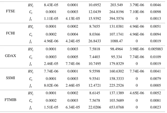
Table 1. The descriptive statistics

Variables Mean

Standard-

errors Skewness

Excess

Kurtosis Min Max

FTSE 𝑅𝑉𝑡 8.43E-05 0.0001 10.6952 203.549 3.79E-06 0.0046 𝐶𝑡 0.0001 0.0003 12.0439 264.8196 7.10E-06 0.0098 𝐽𝑡 1.11E-05 4.13E-05 15.9392 394.5576 0 0.0013 FCHI 𝑅𝑉𝑡 0.0001 0.0002 8.7655 131.0381 4.96E-06 0.0051 𝐶𝑡 0.0002 0.0004 8.0366 107.1741 4.96E-06 0.0094 𝐽𝑡 4.96E-06 4.24E-05 26.8433 1088.47 0 0.0019 GDAX 𝑅𝑉𝑡 0.0001 0.0003 7.5818 98.4964 3.98E-06 0.005883 𝐶𝑡 0.0003 0.0005 7.4403 95.334 7.74E-06 0.0109 𝐽𝑡 2.46E-05 7.74E-06 10.7495 179.8329 0 0.0019 SSMI 𝑅𝑉𝑡 7.74E-06 0.0001 9.5598 160.6302 7.74E-06 0.0041 𝐶𝑡 0.0001 0.0003 9.5541 158.3333 0 0.0079 𝐽𝑡 8.02E-06 2.46E-05 12.4721 225.2526 0 0.0005 FTMIB 𝑅𝑉𝑡 0.0001 0.0002 8.6145 137.1389 4.65E-06 0.0052 𝐶𝑡 0.0002 0.0003 7.5678 103.5689 0 0.0081 𝐽𝑡 1.51E-05 6.34E-05 22.0206 653.0768 0 0.0023

For all the series, the skewness coefficients differ from zero and are positive, indicating a right-skewed distribution. In addition, the excess kurtosis indicates a leptokurtic distribution with values concentrated around the mean and fat tails for all series. RVFTSE 2000 2001 2002 2003 2004 2005 2006 2007 2008 2009 2010 2011 2012 2013 2014 2015 2016 2017 0.000 0.001 0.002 0.003 0.004 0.005

(7)

2667

|

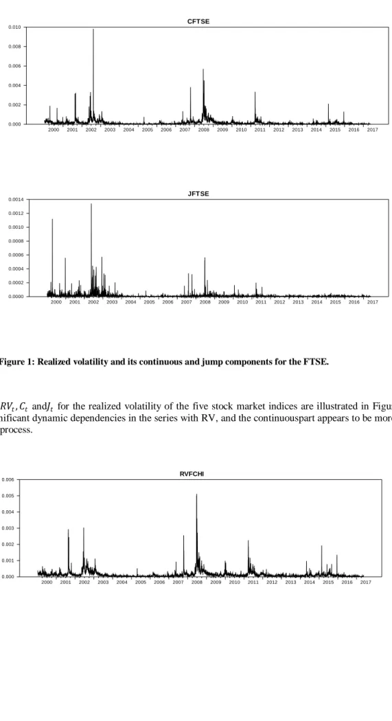
Figure 1: Realized volatility and its continuous and jump components for the FTSE.

Plots of 𝑅𝑉𝑡, 𝐶𝑡 and𝐽𝑡 for the realized volatility of the five stock market indices are illustrated in Figures 1 to 5. These

revealsignificant dynamic dependencies in the series with RV, and the continuouspart appears to be more predictablethan the jump process.

CFTSE 2000 2001 2002 2003 2004 2005 2006 2007 2008 2009 2010 2011 2012 2013 2014 2015 2016 2017 0.000 0.002 0.004 0.006 0.008 0.010 JFTSE 2000 2001 2002 2003 2004 2005 2006 2007 2008 2009 2010 2011 2012 2013 2014 2015 2016 2017 0.0000 0.0002 0.0004 0.0006 0.0008 0.0010 0.0012 0.0014 RVFCHI 2000 2001 2002 2003 2004 2005 2006 2007 2008 2009 2010 2011 2012 2013 2014 2015 2016 2017 0.000 0.001 0.002 0.003 0.004 0.005 0.006

(8)

2668

|

Figure 2: Realized volatility and its continuous and jump components for the FCHI.

The different jump components take positive values on an almost daily basis, which contrasts with the conventional notion that jumps occur rarely. These jumps seem to correspond with notable events on the stock markets. The first common jump coincides with when the dotcom bubble, also known as the Internet bubble, which reached its peak in March 2000, resultingin a huge overvaluation in the stock market.

CFCHI 2000 2001 2002 2003 2004 2005 2006 2007 2008 2009 2010 2011 2012 2013 2014 2015 2016 2017 0.000 0.002 0.004 0.006 0.008 0.010 JFCHI 2000 2001 2002 2003 2004 2005 2006 2007 2008 2009 2010 2011 2012 2013 2014 2015 2016 2017 0.00000 0.00025 0.00050 0.00075 0.00100 0.00125 0.00150 0.00175 0.00200 RVGDAX 2000 2001 2002 2003 2004 2005 2006 2007 2008 2009 2010 2011 2012 2013 2014 2015 2016 2017 0.000 0.001 0.002 0.003 0.004 0.005 0.006

(9)

2669

|

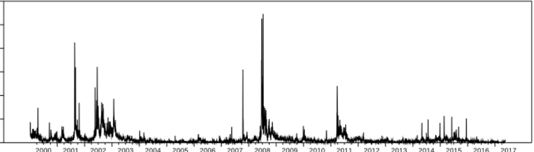
Figure 3: Realized volatility and its continuous and jump components for the GDAX.

The second common jumps between 2001 and 2002 coincide with fluctuations in the forex market following the emergence of the euro and the depreciation of the US dollar. The subprime crisis and the subsequent sovereign debt crisis in the Eurozone explain the jumps in 2008 and 2010.

CGDAX 2000 2001 2002 2003 2004 2005 2006 2007 2008 2009 2010 2011 2012 2013 2014 2015 2016 2017 0.000 0.002 0.004 0.006 0.008 0.010 0.012 JGDAX 2000 2001 2002 2003 2004 2005 2006 2007 2008 2009 2010 2011 2012 2013 2014 2015 2016 2017 0.00000 0.00025 0.00050 0.00075 0.00100 0.00125 0.00150 0.00175 0.00200

(10)

2670

|

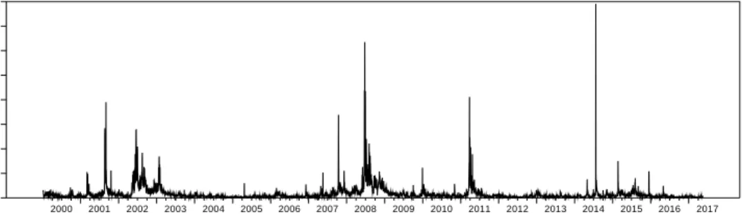
Figure 4: Realized volatility and its continuous and jump components for the SSMI.

The different stock market indices incorporated many international and overseas corporations, thus exposing the indices to currency fluctuations and global trends.

CSSMI 2000 2001 2002 2003 2004 2005 2006 2007 2008 2009 2010 2011 2012 2013 2014 2015 2016 2017 0.000 0.001 0.002 0.003 0.004 0.005 0.006 0.007 0.008 JSSMI 2000 2001 2002 2003 2004 2005 2006 2007 2008 2009 2010 2011 2012 2013 2014 2015 2016 2017 0.0000 0.0001 0.0002 0.0003 0.0004 0.0005 0.0006

(11)

2671

|

Figure 5: Realized volatility and its continuous and jump components for the FTMIB.

4. Results

In this section, we compare the performance of the HAR-RV and HAR-RV-CJ models for the considered stock indices. We forecast the last year for each index and evaluate the predictionsusingMincer-Zarnowitz regressions.

4.1 HAR-RV vs. HAR-RV-CJ

To evaluate the relative performances of the HAR-RV and HAR-RV-CJ models, we forecast the last year for each stock index and subsequently evaluated this using Mincer-Zarnowitz regressions. Furthermore, we focused on the logarithmic versions of the HAR-RV and HAR-RV-CJ models.

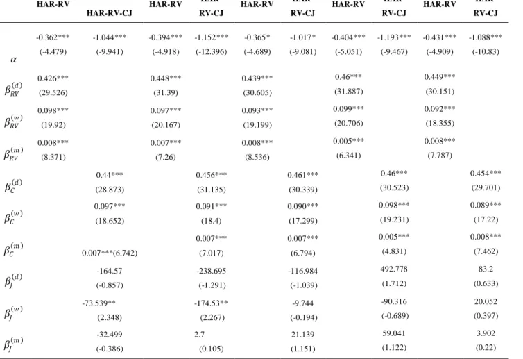
According to the empirical estimates in Table 4, we can see that the estimated coefficients of the HAR-RV model and the continuous estimated coefficients of the HAR-RV-CJ model for the considered series are significant with a decreasing magnitude over the time horizon. The daily impact is greater than the weekly impact, which is in turn greater than the monthly impact. These results agree with the long run dependence property describing the stock realized volatility indices process. For the FTSE and FCHI series, we found that the weekly coefficients corresponding to the jump components is significant and negative, indicating that the jumps may tend to decrease future volatility and its persistence, and this is consistent with the results of Andersen et al. (2007). For the GDAX, SSMI, and FTMIB series, we see that the parameters corresponding to the jump components are not significant, indicating the dominance of the continuous part. We can therefore assume that most of the jump coefficient estimates are insignificant, indicating the poor predictive potential of jumps. Indeed, the predictability in the HAR-RV realized volatility model is likely to be largely due to the continuous sample path components.

CFTMIB 2000 2001 2002 2003 2004 2005 2006 2007 2008 2009 2010 2011 2012 2013 2014 2015 2016 2017 0.000 0.001 0.002 0.003 0.004 0.005 0.006 0.007 0.008 0.009 JFTMIB 2000 2001 2002 2003 2004 2005 2006 2007 2008 2009 2010 2011 2012 2013 2014 2015 2016 2017 0.0000 0.0005 0.0010 0.0015 0.0020 0.0025

(12)

2672

|

Table 2.Estimation results for the HAR-RV and HAR-RV-CJ models

LRV FTSE LRV FCHI LRV GDAX LRV SSMI LRV FTMIB

HAR-RV HAR-RV-CJ HAR-RV HAR-RV-CJ HAR-RV HAR-RV-CJ HAR-RV HAR-RV-CJ HAR-RV HAR-RV-CJ 𝛼 -0.362*** (-4.479) -1.044*** (-9.941) -0.394*** (-4.918) -1.152*** (-12.396) -0.365* (-4.689) -1.017* (-9.081) -0.404*** (-5.051) -1.193*** (-9.467) -0.431*** (-4.909) -1.088*** (-10.83) 𝛽_𝑅𝑉 𝑑 0.426*** (29.526) 0.448*** (31.39) 0.439*** (30.605) 0.46*** (31.887) 0.449*** (30.151) 𝛽𝑅𝑉 𝑤 0.098*** (19.92) 0.097*** (20.167) 0.093*** (19.199) 0.099*** (20.706) 0.092*** (18.355) 𝛽_𝑅𝑉 𝑚 0.008*** (8.371) 0.007*** (7.26) 0.008*** (8.536) 0.005*** (6.341) 0.008*** (7.787) 𝛽_𝐶 𝑑 0.44*** (28.873) 0.456*** (31.135) 0.461*** (30.339) 0.46*** (30.523) 0.454*** (29.701) 𝛽_𝐶 𝑤 0.097*** (18.652) 0.091*** (18.4) 0.090*** (17.299) 0.098*** (19.231) 0.089*** (17.22) 𝛽_𝐶 𝑚 _{0.007***(6.742)} 0.007*** (7.017) 0.007*** (6.794) 0.005*** (4.831) 0.008*** (7.462) 𝛽_𝐽 𝑑 -164.57 (-0.857) -238.695 (-1.291) -116.984 (-1.039) 492.778 (1.712) 83.2 (0.633) 𝛽_𝐽 𝑤 -73.539** _(2.348) -174.53** _(2.267) _(-0.194)-9.744 -90.316 (-0.689) 20.052 (0.397) 𝛽_𝐽 𝑚 _(-0.386)-32.499 2.7 _(0.105) _(1.151)21.139 59.041 (1.122) 3.902 (0.22) R² 0.775 0.786 0.759 0.766 0.763 0.769 0.779 0.781 0.74 0.748 Log-l. -3105.686 -3095.338 -3039.307 -3034.076 -3362.131 -3340.222 -2557.941 -2432.757 -3023.882 -3021.341

Note:The estimated parameters for the daily (d), weekly (w) and monthly (m) components of the RV and HAR-RV-CJ modelsare reported with standard errors.*, **, and *** denote significance at the 10%, 5%, and 1% levels, respectively.

Furthermore, we observe that the parameters for the continuous part of the HAR-RV-CJ model are very close to those for the HAR-RV model. For all the series, the HAR-RV-CJ models bring about a small rise in the R²value when compared to the HAR-RV models. Hence, based on this, the HAR-RV-CJ model appears to fit the data better than the HAR-RV model,thus providing a slightly more accurate estimate.In addition, we can venture to say that the continuous sample path fluctuations have a great impact on the total future volatility movements among the stock markets.

(13)

2673

|

Table 3. Results of the Mincer-Zarnowitz regression test

HAR-RV HAR-RV-CJ HAR-RV HAR-RV-CJ HAR-RV HAR-RV-CJ HAR-RV HAR-RV-CJ HAR-RV HAR-RV-CJ 𝛼 0.115 (0.076) 0.082 (0.075) 0.128 (0.079) 0.110 (0.079) 0.081 (0.082) 0.052 (0.082) 0.102 (0.077) 0.063 (0.076) 0.020 (0.070) 0.008 (0.068) 𝛽 0.938** (0.026) 0.952** (0.023) 0.914** (0.032) 0.917** (0.032) 0.867** (0.043) 0.870** (0.041) 0.845** (0.042) 0.856** (0.043) 0.907** (0.025) 0.930** (0.029) R² 0.635 0.667 0.682 0.694 0.670 0.681 0.630 0.642 0.670 0.690 Log-l -216.746 -203.387 -180.115 -177.098 -202.523 -196.381 -207.429 -193.572 -202.438 -190.442

Note:Estimated parameters evaluating one-year, out-of-sample forecasts of the HAR-RV and HAR-RV-CJ models are reported with standard errors in parentheses. *, **, and *** denote significance at the 10%, 5%, and 1% levels, respectively.

The results of the Mincer-Zarnowitz regressions are shownin Table 3, and they indicate that the HAR-RV-CJ model seems to give more accurate forecasts than the HAR-RV model for the different stock market indices being considered.

4.2 Forecasts results

We perform out-of-sample forecasts foreach stock index’s realized volatility usingpre-forecast periods of variouslength. We first dividedeach stock index’s dataset into a section representing the last year of the dataset and another corresponding tothe pre-forecast period.We then estimate the parameters of the model for pre-forecast periodsof different durations and then produce a forecast for the last year’s realized volatility foreach stock market index.The different pre-forecast periods comprised the last 1, 2, 3, and 5 years, as well as the entire period.

Table 4. Results of forecast evaluation

MSE Theil’s U MSE Theil’s U MSE Theil’s U MSE Theil’s U MSE Theil’s U

1 3.45e-04 0.8562 0.0002 0.6324 0.0002 1.2037 1.86e-05 0.4802 0.0001 0.8615 2 1.18e-04 0.6113 0.001 1.4462 0.0007 1.277 0.00006 1.2684 0.0004 0.9768 3 2.01e-04 0.6951 0.0001 0.3517 1.45e-04 0.6685 0.00004 0.7641 0.0005 1.0524 5 4.95e-04 1.0638 0.0002 0.8234 0.0003 1.4658 0.00005 0.8581 0.0008 1.2580 A ll 5.26e-04 2.8625 0.003 4.4549 0.002 3.6436 0.0001 2.1232 0.0004 3.7129

Note:Forecast evaluation statistics comparing the accuracy of one-year, out-of-sample forecasts depending on the length of pre-forecast period

Table 4 presents statistics that illustrate the performance of the forecasts. For the SSMI series, the best forecast is based on the model estimated using the two previous years, with the worst forecast being based on the whole period. For both the FCHI and GDAXseries, the MSE and Theil’s U suggest that the forecast based on the previous three years is the best, while the forecast based on the whole period is the worst. For both the SSMI and FTMIB series, the best forecast is achieved with the model estimated using just the previous year, with the worst forecast again being based on the whole period. This progressive deterioration in performance with longer forecast periods contrasts with the notion that estimated parameters are more accurate with more data. One plausible explanation for this could be that extreme events occurred during the forecast period (e.g., crises, shocks, news), and these affected the evolution of volatility in the stock market.

(14)

2674

|

5. Conclusion

This study sought to investigate how decomposing the realized variance into its continuous and jump components could improve the predictability of realized volatility in stock markets. We built our methodology based on the heterogeneous autoregressive model with the various components of volatility and applied it to high-frequency data. The empirical results suggest that volatility jumps have a negative effect on the persistent component of volatility, which is in accordance with the findings of Anderson et al. (2007). It is also clear from the estimation results that this effect is attenuated over time.

The empirical results reveal that jump dynamics are much less predictable when compared to continuous sample path dynamics. Moreover, the use of high-frequency data enables us to capture many more jumps than models based on daily data. In addition, it seems that many significant jumps are related to historical events or announcements of macroeconomic news. Finally, incorporating the continuous sample path and jump component measures in the volatility forecasting model ensures that the continuous part has a relevant predictive power.

We compared the forecasting abilities of the HAR-RV and HAR-RV-CJ models and found that the HAR-RV-CJ model surpassed the HAR-RV model when modeling the realized volatility of the stock market indices. However, the forecast results for the SSMI and FTMIB series suggest that realized volatility forecasts are better when based on a very short pre-forecast period of just one year. We could therefore consider that the HAR model is perhaps not the most appropriate choice for modeling the realized volatility of these two stock markets, implying that volatility appears to manifest differently in different stock markets.

The empirical results may be considered indicative of numerous attractive avenues for further research. First, it appears that modeling and predicting the continuous sample path and jump components of the quadratic variation process separately may improve pricing decisions. Second, empirical observation shows that jumps appear habitually and instantaneously among different markets, which suggests that it may be interesting to extend the present study to a multivariate framework.

References

[1] Andersen, Torben G, and Tim Bollerslev. 1998. "Deutsche mark–dollar volatility: intraday activity patterns, macroeconomic announcements, and longer run dependencies." the Journal of Finance no. 53 (1):219-265.

[2] Andersen, Torben G, Tim Bollerslev, and Francis X Diebold. 2007. "Roughing it up: Including jump components in the measurement, modeling, and forecasting of return volatility." The Review of Economics and Statistics no. 89 (4):701-720.

[3] Andersen, Torben G, Tim Bollerslev, Francis X Diebold, and Paul Labys. 2003. "Modeling and forecasting realized volatility." Econometrica no. 71 (2):579-625.

[4] Andersen, Torben G, Tim Bollerslev, and Xin Huang. 2011. "A reduced form framework for modeling volatility of speculative prices based on realized variation measures." Journal of Econometrics no. 160 (1):176-189.

[5] Barndorff-Nielsen, Ole E, and Neil Shephard. 2004. "Power and bipower variation with stochastic volatility and jumps." Journal of financial econometrics no. 2 (1):1-37.

[6] Barndorff-Nielsen, Ole E, and Neil Shephard. 2006. "Econometrics of testing for jumps in financial economics using bipower variation." Journal of financial Econometrics no. 4 (1):1-30.

[7] Barunik, Jozef, Tomas Krehlik, and Lukas Vacha. 2016. "Modeling and forecasting exchange rate volatility in time-frequency domain." European Journal of Operational Research no. 251 (1):329-340.

[8] Beine, Michel, Jérôme Lahaye, Sébastien Laurent, Christopher J Neely, and Franz C Palm. 2007. "Central bank intervention and exchange rate volatility, its continuous and jump components." International journal of finance & economics no. 12 (2):201-223.

[9] Bollerslev, T., Engle, R. F., & Nelson, D. B. (1994). ARCH models. Handbook of econometrics, 4, 2959-3038.

[10]Bollerslev, Tim, Uta Kretschmer, Christian Pigorsch, and George Tauchen. 2009. "A discrete-time model for daily S & P500 returns and realized variations: Jumps and leverage effects." Journal of Econometrics no. 150 (2):151-166.

[11]Busch, T., Christensen, B. J., & Nielsen, M. Ø. (2011). The role of implied volatility in forecasting future realized volatility and jumps in foreign exchange, stock, and bond markets. Journal of Econometrics, 160(1), 48-57.

(15)

2675

|

[12]Corsi, Fulvio. 2009. "A Simple Approximate Long-Memory Model of Realized Volatility." Journal of Financial Econometrics no. 7 (2):174-196.

[13]Corsi Fulvio, Davide Pirino, and Roberto Reno. 2010. "Threshold bipower variation and the impact of jumps on volatility forecasting." Journal of Econometrics 159 (2): 276-288.

[14]Degiannakis*, S. (2004). Volatility forecasting: evidence from a fractional integrated asymmetric power ARCH skewed-t model. Applied Financial Economics, 14(18), 1333-1342.

[15]Degiannakis, S. A. (2008). Forecasting Vix. Journal of Money, Investment and Banking, (4).

[16]Fernandes, M., Medeiros, M. C., & Scharth, M. (2014). Modeling and predicting the CBOE market volatility index. Journal of Banking & Finance, 40, 1-10.

[17]French, Kenneth R, G William Schwert, and Robert F Stambaugh. 1987. "Expected stock returns and volatility."

Journal of financial Economics no. 19 (1):3-29.

[18]Fuentes, M. A., Gerig, A., & Vicente, J. (2009). Universal behavior of extreme price movements in stock markets.

PloS one, 4(12).

[19]Hansen, P. R., & Lunde, A. (2005). A forecast comparison of volatility models: does anything beat a GARCH (1, 1)?. Journal of applied econometrics, 20(7), 873-889.

[20]Huang, Chuangxia, Xu Gong, Xiaohong Chen, and Fenghua Wen. 2013. "Measuring and forecasting volatility in Chinese stock market using HAR-CJ-M model." In Abstract and Applied Analysis, vol.2013. Hindawi.

[21]Koopman, Siem Jan, Borus Jungbacker, and Eugenie Hol. 2005. "Forecasting daily variability of the S&P 100 stock index using historical, realised and implied volatility measurements." Journal of Empirical Finance no. 12 (3):445-475.

[22]Kumar Manish. 2010. "Improving the accuracy: volatility modeling and forecasting using high-frequency data and the variational component." Journal of Industrial Engineering and Management (JIEM) 3 (1): 199-220.

[23]Lanne, Markku. 2007. "Forecasting realized exchange rate volatility by decomposition." International Journal of Forecasting no. 23 (2):307-320.

[24]Martens, Martin. 2001. "Forecasting daily exchange rate volatility using intraday returns." Journal of International Money and Finance no. 20 (1):1-23.

[25]Müller, Ulrich A., Michel M. Dacorogna, Rakhal D. Davé, Richard B. Olsen, Olivier V. Pictet, and Jacob E. von Weizsäcker. 1997. "Volatilities of different time resolutions — Analyzing the dynamics of market components."

Journal of Empirical Finance no. 4 (2):213-239.

[26]Pooter, Michiel de, Martin Martens, and Dick van Dijk. 2008. "Predicting the daily covariance matrix for s&p 100 stocks using intraday data—but which frequency to use?" Econometric Reviews no. 27 (1-3):199-229.