Open Research Online
The Open University’s repository of research publications
and other research outputs
Forecasting multivariate road traffic flows using
Bayesian dynamic graphical models, splines and other
traffic variables
Journal Item
How to cite:
Anacleto Junior, Osvaldo; Queen, Catriona and Albers, Casper (2013). Forecasting multivariate road traffic flows using Bayesian dynamic graphical models, splines and other traffic variables. Australian & New Zealand Journal of Statistics, 55(2) pp. 69–86.
For guidance on citations see FAQs.
c
2013 Australian Statistical Publishing Association Inc. Version: Accepted Manuscript
Link(s) to article on publisher’s website: http://dx.doi.org/doi:10.1111/anzs.12026
Copyright and Moral Rights for the articles on this site are retained by the individual authors and/or other copyright owners. For more information on Open Research Online’s data policy on reuse of materials please consult the policies page.
Forecasting multivariate road traffic flows using
Bayesian dynamic graphical models, splines and other
traffic variables
Osvaldo Anacleto
∗Department of Mathematics and Statistics, The Open University
Catriona Queen
Department of Mathematics and Statistics, The Open University
Casper Albers
Department of Psychometrics and Statistics, University of Groningen
Abstract
Traffic flow data are routinely collected for many networks worldwide. These in-variably large data sets can be used as part of a traffic management system, for which good traffic flow forecasting models are crucial. The linear multiregression dynamic model (LMDM) has been shown to be promising for forecasting flows, accommodat-ing multivariate flow time series, while beaccommodat-ing a computationally simple model to use. While statistical flow forecasting models usually base their forecasts on flow data alone, data for other traffic variables are also routinely collected. This paper shows how cubic splines can be used to incorporate extra variables into the LMDM in order to enhance flow forecasts. Cubic splines are also introduced into the LMDM to parsimoniously accommodate the daily cycle exhibited by traffic flows.
The proposed methodology allows the LMDM to provide more accurate forecasts when forecasting flows in a real high-dimensional traffic data set. The resulting ex-tended LMDM can deal with some important traffic modelling issues not usually con-sidered in flow forecasting models. Additionally the model can be implemented in a real-time environment, a crucial requirement for traffic management systems designed to support decisions and actions to alleviate congestion and keep traffic flowing.
Keywords: linear multiregression dynamic model, dynamic linear model, state space models,
cubic splines, occupancy, headway, speed.
∗Corresponding author ([email protected]). The authors thank the Highways Agency for
providing the data used in this paper and also Les Lyman from Mott MacDonald for valuable discussions on preliminary data analyses. The authors also would like to thank two Referees for their constructive and helpful comments on an earlier version of the paper.
1
Introduction
Traffic flow data are routinely collected across many traffic networks worldwide. These data sets are invariably very large with variables measured at a number of data collection sites S(1), . . . , S(n), very often collected minute-by-minute over long periods of time. These time series data can be used as part of a traffic management system to assess highway facilities and performance over time or to monitor and control traffic flows in real-time. They can also be used as part of a traveller’s information system. The success of such systems relies on good short-term forecasting models of flows and it is the development of such models which is considered in this paper.
Despite the fact that traffic flow data are invariably multivariate — often of high dimen-sion — many authors model the flow at each site in isolation. However, the flows at upstream
and downstream sites are very informative about the flows at S(i) and there are substantial
gains to be made by using this information when forecasting flows. Some authors (Tebaldi
et al., 2002; Kamarianakis and Prastacos, 2005; Stathopoulos and Karlaftis, 2003) do use
other flows to help forecast flows at each S(i), while others (Whittaker et al., 1997; Sun et
al., 2006) additionally use conditional independence so that only the flows at sites adjacent
to S(i) are required to help forecast flows at S(i). However, these authors use lagged flows,
whereas, as shown in Anacleto et al. (2013), when the distances between sites are such that
vehicles are counted at several different sites within the same time period — as they are in
the network considered in this paper — then using information regarding contemporaneous
flows can greatly improve forecast performance.
Following the traffic flow modelling ideas of Queen et al. (2007), Queen and Albers
(2009) and Anacletoet al. (2013), this paper uses a multivariate Bayesian dynamic graphical
model called the linear multiregression dynamic model (LMDM) (Queen and Smith, 1993) to forecast flows. Instead of using lagged flow information, the LMDM uses contemporaneous
upstream flow information at time t to forecast flows at site S(i) at the same time t (by
marginalising the forecast distribution for S(i) at time t - see Section 3 for details). The LMDM can accommodate the high-dimensional, often complex, multivariate relationships which can exist between flow series across networks, and yet, because it uses a graph to decompose the problem into smaller, simpler sub problems, it is a computationally simple
model to use, making it an ideal candidate for on-line traffic forecasting.
Statistical flow forecasting models usually base their forecasts on flow data alone. How-ever, data for other traffic variables — namely, occupancy, headway and speed — are also routinely collected for many roads. Each of these variables has a non-linear relationship with flow. This paper investigates how cubic splines can be used to incorporate these extra traffic variables into the LMDM. The paper also introduces the use of cubic splines within the LMDM to accommodate seasonal patterns, and in particular, to accommodate the daily cycle exhibited by traffic flows. The proposed models are used in the paper to forecast traffic flows at a busy motorway intersection near Manchester, UK.
Although the paper focuses on the problem of forecasting traffic flows, the proposed model has much wider applicability to any application involving multivariate time series which exhibits a causal structure and, as such, the methodology presented in the paper is of interest in its own right.
The paper is structured as follows. Section 2 describes the data used throughout the paper. Section 3 gives a brief review of the LMDM and describes how cubic splines can be used within the LMDM in order to accommodate the daily cycle exhibited by traffic flows. In Section 4, cubic splines are also used to model the non-linear relationships which exist between the extra traffic variables and flows. These cubic splines are then incorporated into the LMDM so that information regarding the extra traffic variables can be used when forecasting flows. Section 5 goes on to assess the forecast performance of these models, while Section 6 offers some concluding remarks.
2
The data
This paper focuses on forecasting traffic flows at the intersection of three motorways — the M60, M62 and M602 — west of Manchester, UK. Figure 1(a) shows a schematic diagram of the network with arrows showing the direction of travel and circles indicating the data collection sites. The data used in the paper were collected in 2010 by the Highways Agency in England (http://www.highways.gov.uk/).
FIGURE 1 ABOUT HERE
in the surface of the road at each site (for a brief description of the data collection process by inductive loops, see Li, 2009). Even though minute counts are available, because of the high variability of these, researchers usually aggregate the data (Vlahogianniet al., 2004 and
Chandra and Al-Deek, 2009). Anacleto et al. (2013), who developed models for forecasting
flows in this same Manchester network using the same data as here, aggregated the flows into 15-minute intervals, making the data and their models particularly useful for assessing highway facilities and for providing traveller information. In this paper, the focus is on real-time traffic control for which 5-minute intervals are suitable, and so the data will be aggregated into 5 minute intervals here.
Figure 1(b) shows 5-minute flow time series plots for sites 9206B and 1437A for a typical week. Notice the morning and afternoon peaks at both sites, which are also evident at all
other sites in the network. As was shown in Anacletoet al. (2013), flows in this network vary
in level and variability for different weekdays. These differences can be incorporated into the model, but for clarity, in this paper only data for Wednesdays are considered. Further, the very low overnight flows (which are of little interest for real-time traffic control) are ignored and only data between 06:00-20:59 are used.
As mentioned in the introduction, the distances between sites in this network are such that vehicles are usually counted at several data sites in the same 5-minute interval. As a result, the flows at sites upstream to siteS(i) at timetare helpful in forecasting the flows at S(i) at the same time t. It would, of course, be easier to use lagged upstream flows (which
are known at time t) for forecasting at time t rather than contemporaneous upstream flows
(which are not known at time t). However, Anacleto et al. (2013) found that for both
15-minute and 5-15-minute data in this network, a model which used contemporaneous upstream flows within an LMDM performed better than a model using lagged flows.
In addition to the flow data, there are data for three other variables collected at each site:
• Occupancy: the percentage of time that vehicles are ‘occupying’ the inductive loop;
• Headway: the average time between vehicles passing over the inductive loop (in sec);
• (Time mean) speed: the average ratio of the distance between two (consecutive)
FIGURE 2 ABOUT HERE loops (in kph).
These data are available minute-by-minute and averaged into 5-minute values for considering with 5-minute flow data.
3
The model
This section describes the LMDM used for 5-minute flow data in the Manchester network. For a detailed description of the LMDM, see Queen and Smith (1993).
Denote the flow atS(i) during time periodtbyYt(i). Suppose that there are conditional independence relationships related to causality across Yt(1), . . . , Yt(n) so that for eachYt(i), i = 2, . . . , n, there is a set of variables, pa(Yt(i)) ⊆ {Yt(1), . . . , Yt(i−1)}, for which, condi-tional on the set of variablespa(Yt(i)),Yt(i) is independent of{Yt(1), . . . , Yt(i−1)}\pa(Yt(i))
(where “\” reads “excluding”). These relationships can be represented by a directed acyclic
graph (DAG) in which there are directed arcs to Yt(i) from each variable inpa(Yt(i)). Each variable inpa(Yt(i)) is known as aparent ofYt(i) whileYt(i) in turn is achild of each variable in pa(Yt(i)). If pa(Yt(i)) =∅, then Yt(i) is known as a root node.
In Anacleto et al. (2013), a DAG was elicited for the Manchester network using the
directions of traffic flows and possible routes through the network: the final DAG used in that paper, which will also be used in this paper, is shown in Figure 2.
The LMDM uses the DAG to model the n-dimensional multivariate time series by n
separate (conditional) univariate Bayesian regression dynamic linear models (DLMs) (West
and Harrison, 1997). Let Dt−1 denote the information available at time t −1. Then the
LMDM is defined as follows for all times t= 1,2, . . .:
Yt(i) = Ft(i)>θt(i) +vt(i), vt(i)∼N(0, Vt(i)), i= 1, . . . , n, (1)
θt = Gtθt−1+wt, wt∼N(0,Wt), (2)
θt−1|Dt−1 ∼ N(mt−1,Ct−1). (3)
where the vector Ft(i) contains an arbitrary, but known, function of the parents pa(Yt(i)) and possibly other known variables; θt(i) is the state vector associated with Yt(i) andθ>t =
(θt(1)> · · · θt(n)>);vt(1), . . . , vt(n) are the observation errors,Vt(1), . . . , Vt(n) are the scalar
observation variances; the square matrices Gt = blockdiag(Gt(1) · · · Gt(n)) and Wt =
blockdiag(Wt(1) · · · Wt(n)) are such that Gt(i) and Wt(i) are, respectively, the state evolution matrix and evolution covariance matrix for θt(i); w>t = (wt(1)> . . . wt(n)>)
where wt(i) is the system error vector for Yt(i); 0 is a vector of zeros; and vectormt−1 and
square matrix Ct−1 = blockdiag(Ct−1(1) · · · Ct−1(n)) are the posterior moments for θt−1.
The errors vt(1), . . . , vt(n) andwt(1), . . . ,wt(n) are mutually independent of each other and through time.
At each timet, given the posterior distribution for θt−1|Dt−1 in (3), the prior forθt|Dt−1
is obtained via the system equation (2) and, in turn, the forecast distribution for each Yt(i)|pa(Yt(i)), Dt−1 is obtained from the observation equations (1). The block diagonal
forms of Wt and Gt ensure that if the state vectors are initially mutually independent,
then they remain so for all time t. Basically, the LMDM specifies n separate (conditional)
univariate models — one each for Yt(1) and Yt(i)|pa(Yt(i)),i= 2, . . . , n— where each Yt(i) has a function of its parents as linear regressors and its associated state vector, θt(i), is
updated separately in closed form in Yt(i)’s (conditional) univariate model. Root nodes
without parents are modelled by any suitable univariate DLM.
From (1), the forecast distribution for each Yt(i)|pa(Yt(i)) is normal and can be ob-tained separately within the LMDM. However, as Yt(i) and pa(Yt(i)) both represent flows
at the same time t, the marginal forecasts for each Yt(i) are required. Although the
marginal forecast distributions cannot generally be calculated analytically, the marginal forecast moments are readily available using E[Yt(i)] =E{E[Yt(i)|pa(Yt(i))]}and V[Yt(i)] = E{V[Yt(i)|pa(Yt(i))]}+V{E[Yt(i)|pa(Yt(i))]}. Essentially, in the LMDM, the marginal fore-cast moments of flows at upstream sites are used to obtain the marginal forefore-cast moments
for Yt(i), which in turn are used to find the marginal forecast moments of sites further
downstream, and so on (see Queen and Smith, 1993 and Queen et al., 2008).
The observation variances Vt(1), . . . , Vt(n) in (1) are estimated on-line as data are
ob-served using a method proposed by Anacletoet al. (2013) to accommodate the
heteroscedas-ticity exhibited by time series of traffic flows. Briefly, each Vt(i) is replaced by
where α is such that
log(variance of flow) = αlog(mean flow)
and can be estimated using historical data (this relationships is different for the two periods
7.00pm–6.59am and 7.00am–6.59pm and so α takes one value for t between 7.00pm and
6.59am each day, and a different value between 7.00am and 6.59pm); E(Yt(i)|Dt−1) is the
one-step ahead forecast mean for Yt(i); and φt(i) is the underlying observation precision which is estimated on-line using the discounting variance learning techniques described in West and Harrison (1997), page 359.
The matricesWt(1), . . . ,Wt(n) are also estimated on-line using standard DLM discount-ing techniques (see West and Harrison, 1997, page 193).
Because of the heteroscedasticity of traffic flow time series, when evaluating model fore-cast performance it is important to consider the performance of the precision of forefore-casts as well as point forecasts. Thus, a measure which assesses the accuracy of the multivariate forecast distribution as a whole, rather than just the point forecasts, is preferred. Such a measure is the joint log-predictive likelihood (LPL). After observing the time series up to
time T, the LPL evaluates the log of the density of the joint one-step ahead forecast
dis-tribution at time t at the observed value y>t = (yt(1), . . . , yt(n)), and aggregates these over
all values t = 1, . . . , T. In the LMDM, because of the conditional independence structure
across Yt(1), . . . , Yt(n), the density of the joint one-step ahead forecast distribution at time t evaluated at the observed value yt is given by
f(yt|Dt−1) =
n Y
i=1
f(yt(i)|pa(yt(i)), Dt−1)
where f(yt(i)|pa(yt(i)), Dt−1) is the one-step forecast density for Yt(i) conditional on its
parents, evaluated at yt(i). Thus, the LPL for the LMDM is calculated as
LPL = T X t=1 " n X i=1 log{f(yt(i)|pa(yt(i)), Dt−1)} # . (5)
The larger the value of the LPL, the more support there is for the corresponding model. The forecast densities in (5) are calculated at time t−1 before yt(i) is observed. Therefore, the LPL is not subject to overfitting problems which may affect model comparison.
3.1
Modelling the daily cycle
In the LMDM of Anacleto et al. (2013), the daily cycle observed in flows at root nodes
was modelled using a seasonal factor representation so that θt(i) in (1) is a 96-dimensional vector of flow level parameters (one mean flow level parameter for each 15-minute period in the day) with corresponding 96-dimensional vector Ft(i)> = (1 0 . . . 0). (The matrix
Gt in (2) then ‘cycles’ through the mean level parameters to ensure that the correct
15-minute mean flow level parameter is used at timet.) Child series have their parents as linear regressors, where the regression coefficients represent the proportions of vehicles flowing from parent to child. These proportions also exhibit a daily pattern, also modelled by a seasonal factor representation in Anacleto et al. (2013) so that, for a series with a single parent (for simplicity), once again θt(i) in (1) is a 96-dimensional vector of proportion parameters with corresponding 96-dimensional vector Ft(i)> = (pa(yt(i)) 0 . . . 0).
Unfortunately, when the dimension of the state vector gets large, numerical problems can arise when updating the variances associated with a DLM (Prado and West, 2010). This can be tackled by using alternative equations in the Kalman filter algorithm, as implemented in
theR DLM package (Petriset al., 2009), but when dealing with 5-minute data, the dimension
of the state vector is so large (12×24) that it becomes important to consider alternatives to
the seasonal factor representation to keep model parsimony. Following Tebaldi et al. (2002),
to address this problem splines can be used to represent daily cycles in each univariate DLM within the LMDM.
Cubic splines are widely used in regression models in order to relax the linearity assump-tion for continuous regressors (see Harrell, 2001, and Hastieet al., 2001). A cubic spline has the basic form:
f(x) = M X
m=1
βmhm(x), (6)
where hm(x) = xm for m = 1,2,3 and hm(x) = (x−k
m−3)3 for m = 4, . . . , M for values
k1, ..., kM−3 with a < k1 < k2 < ... < kM−3 < b, where [a, b]∈ R is the domain of x. When
x−km−3 is negative, thenhm(x) = 0. The functionsh1(x), . . . , hM(x) are called spline basis functions, k1, ..., kM−3 are the spline knots and β1, . . . , βM are parameters. In the context of regression, the idea is to consider the spline basis functions as regressor variables and then estimate the parameters β1, . . . , βM.
In a dynamic LMDM context, a similar approach can be used. Consider a root node. The daily cycle can be modelled in a time series using a spline to fit one full cycle. In this case, x would be time t and k1, . . . , kM−3 would represent times over the cycle. For example, for
5-minute data with a daily cycle over 24 hours,k1 could be 13, for example, representing the
time period 01:00–01:04 and t would be the current time (which at 02:00–02:04, say, would
be t = 25). Prior data can be used to calculate the spline basis functions h1(x), . . . , hM(x) which can then be evaluated at each 5-minute time periodx=t. The regression vectorFt(i) for root node Yt(i) in (1) then has the form:
Ft(i)> = (h1(t) · · · hM(t)). (7)
(This form of Ft(i) only models the daily cycle of flows: it is possible that Ft(i) could have
additional elements, for example there may be other exogenous regressors for Yt(i)’s DLM.)
For Ft(i) in (7), the associated state vector in (1) is:
θt(i)>= (βt1 · · ·βtM) (8)
where βt1, . . . , βtM are dynamic versions of the associated parameters in (6), which evolve
through the system equation (2) with state evolution matrix Gt(i) being theM-dimensional
identity matrix.
Although Harrell (2001) suggests that the positions of k1, . . . , kM−3 are not important
when fitting splines for static regression purposes, it was found that LMDMs for traffic flows give better results when concentrating the positions of k1, . . . , kM−3 during morning and
afternoon peak periods. Harrell (2001) also recommends using only 3 to 5 knots for static regression. However, when using splines to represent daily cycles of flows, 15 to 20 knots were typically found to perform much better. This is a small number when compared to the 288 parameters required to use a seasonal factor representation to model 5-min flow data. Moreover, overfitting is controlled because fitted splines were found to not vary very much over time and the parameters βt1, . . . , βtM evolve dynamically to capture any drift in time.
Example 1
Suppose that the daily cycle of root node Yt(1) is to be represented by a spline with
included in Yt(1)’s DLM. Then the observation equation for Yt(1) has the form Yt(1) = 5 X m=1 βtmhm(t) +αtxt+vt(1), vt(1)∼N(0, Vt(1)), so that in (1), Ft(1)> = (h1(t) · · · h5(t) xt) θt(1)> = (βt1 · · · βt5 αt).
In this case the evolution matrix Gt(1) = blockdiag(I5, g) where I5 is the 5-dimensional
identity matrix and g is some scalar in R for parameter αt’s evolution.
A child in the LMDM is modelled as having its parents as linear regressors. For example, if Yt(3) has parents Yt(1) and Yt(2), then the simplest observation equation for Yt(3) would be
Yt(3) =αt(1)yt(1) +αt(2)yt(2) +vt(3), vt(3) ∼N(0, Vt(3))
so that Ft(3)> = (yt(1) yt(2)) and θt(3)> = (αt(1) αt(2)). For traffic flow data, the
regression parameters (αt(1) and αt(2) in the example above) exhibit a daily pattern (see,
for example, Anacleto et al., 2013). A spline can be used to model the daily cycle by setting
each regression parameter to the form PMm=1βtmhm(t). Thus, in general the regression
and state vectors Ft(i) and θt(i) for child variable Yt(i) with (for simplicity) single parent pa(Yt(i)) have the forms:
Ft(i)> = (pa(yt(i))h1(t) · · · pa(yt(i))hM(t)), (9)
θt(i)> = (βt1 · · · βtM). (10)
Again,θt(i) evolves through the system equation (2) with state evolution matrixGt(i) being
the M-dimensional identity matrix. As with the splines for root nodes, it was found that
splines with 15 to 20 knots performed best and, again, overfitting is not a issue since the parameters in (10) are estimated as flows are observed and the proportion splines do not vary much over time.
Example 2
Suppose that Yt(3) has parents Yt(1) and Yt(2) and the daily cycles exhibited by Yt(1) and Yt(2)’s regression parameters are to be represented by splines with three and two knots,
respectively. Suppose further that an exogenous regressor,Zt, is also to be included inYt(3)’s
model. Then the observation equation for Yt(3) has the form
Yt(3) =yt(1) 6 X m=1 βtm(1)hm(t)(1)+yt(2) 5 X m=1 βtm(2)hm(t)(2)+γ tzt+vt(3), vt(3)∼N(0, Vt(3)), so that in (1), Ft(3)> = (h1(t)(1) · · · h6(t)(1) h1(t)(2) · · · h5(t)(2) zt) θt(3)> = (βt(1)1 · · · β (1) t6 β (2) t1 · · · β (2) t5 γt).
In this case the evolution matrix Gt(3) = blockdiag(I6,I5, g) where Ik is thek-dimensional
identity matrix and g is some scalar in R for parameter γt’s evolution.
To take advantage of the computational simplicity of a fully conjugate LMDM, normal priors need to be specified for the state vectors. When using the seasonal factor model for modelling the daily cycle exhibited by regression parameters in the child model (as in
Anacleto et al., 2013), the regression parameters are proportions and so normal priors are
not ideal. However, when using splines to model the regression parameters’ daily cycles (as in this paper), using normal priors is not a problem as the spline regression parameters do not have any restrictions on their values.
In order to compare the performance of using cubic splines and seasonal factors for mod-elling daily cycles in the LMDM, both models were used to forecast four separate bivariate series formed by considering the four root nodes (in Figure 2) together with one of their children each: specifically, the four bivariate series considered were (Yt(9206B), Yt(9200B)), (Yt(6013B), Yt(6007L)), (Yt(9188A), Yt(9193J)) and (Yt(1431A), Yt(1437A)). To also assess whether dynamic estimation of the spline parameters βt1, . . . , βtM (as in (8) and (10)) im-proves forecast performance, forecasts for these four bivariate series were also obtained using a static version of the cubic spline LMDM, by using a system equation (2) with no error
term wt.
Observed flows from July to August 2010 were used to estimate the spline basis functions, form priors for all state vectors and to estimate parameter α for each Vt(i) in equation (4) for these three models (so that each model had the same equivalent priors). One-step ahead forecasts for flows were then obtained for September 2010.
TABLE 1 ABOUT HERE
Each model and each series requires two separate discount factors to be specified: one for estimating φt(i) in (4) and one for estimatingWt. Usually these discount factors are chosen by comparing the forecast accuracy of different models varying discount factor values (as suggested by West and Harrison, 1997). However, the high number of models and the level of complexity makes this optimization a demanding task. For example, the optimization
of the combination of both discount factors for Wt and φt(i) for a child time series would
depend on the optimization of the discount factors for Wt and φt(i) in its parent. Due to
this, based on preliminary tests, the chosen value for the discount factors for both Wt and
φt(i) in all models in this paper was 0.99.
Table 1 shows the LPLs for the three models for each bivariate series. The number of spline basis functions for static and dynamic spline LMDMs varied between 15 and 20 among the considered time series, and the LPL values shown in Table 1 are for the number of basis functions which performed best for each model and each series. In Table 1, the dynamic spline versions of the LMDMs produce the largest LPL values for all bivariate series, indicating that the dynamic spline LMDMs provide the most accurate forecasts.
An alternative parsimonious approach to using cubic splines for modelling the daily cycle would be to use a Fourier representation, as in West and Harrison (1997), Section 8.6. The standard Fourier representation can be used directly for modelling the daily cycle exhibited by the parents, but the model would need to be adapted somewhat for modelling the daily cycle in the proportion regression parameters in the models for child variables. When modelling the four root nodes, however, the Fourier representation was found to perform worse than both the seasonal factor model and the splines, and so Fourier models were not pursued further.
4
Traffic variables as predictor variables in the LMDM
As mentioned in Section 2, the data collection process used by the Highways Agency in Eng-land includes real-time measurement of flow, together with occupancy, speed and headway. Although there is great interest and an extensive literature concerning traffic flow modelling, few models deal with the analysis of flow in conjunction with the other variables. Based on a
FIGURE 3 ABOUT HERE
survey carried out by Vlahogianniet al. (2004), of forty traffic models where flow was consid-ered, just seven used other extra variables, while none considered all three. From a statistical perspective, Ahmed and Cook (1979) and Levin and Tsao (1980) fitted independent ARIMA
models for flow and occupancy forecasting, while Whittaker et al. (1997) tackled a similar
problem using state space models. Neural networks have also been used for modelling flow
in conjunction with other variables, for example in Innamaa (2000), Abdulhai et. al. (1999)
and Gilmore and Abe (1995). Multivariate forecasting of flow, speed and occupancy using
k-nearest neighbour classifiers has also been considered by Clark (2003). More recently,
Chandra and Al-Deek (2009) considered vector autoregressive models to forecast flows using speed as a predictor variable.
In this section, occupancy, speed and headway data will be incorporated into the LMDM to enhance flow forecasts.
4.1
Relationships between flows and other traffic variables
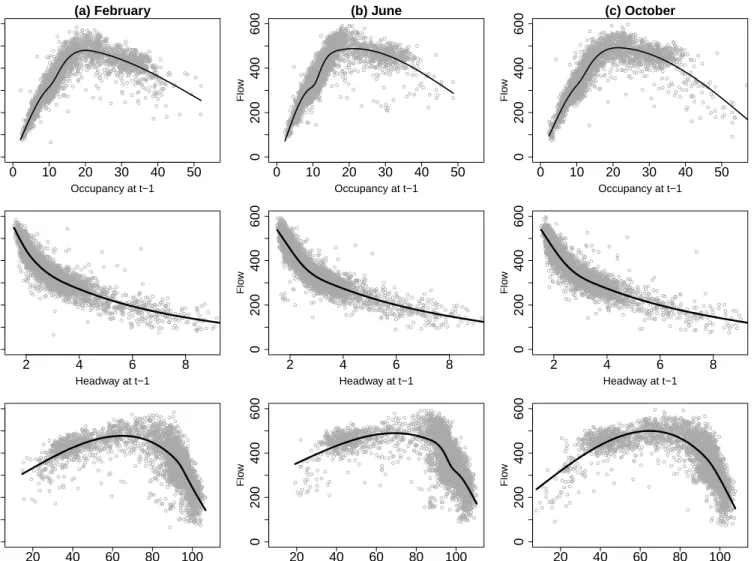
The first row of Figure 3 shows scatterplots of flow at time t versus occupancy at previous
time t−1 at site 9188A for three separate months. The plots indicate an increasing
rela-tionship between flow and occupancy until the latter reaches some value around 20, which is usually defined by traffic managers as the road capacity and varies from site to site. For occupancy values higher than this road capacity, the relationship then turns to be decreas-ing, which can lead to congestion. This relationship, first observed by Greenshields (1935), is well known in the traffic literature and is usually called the fundamental diagram of traffic (for details, see Ashton, 1966).
Scatterplots of flow at timet versus headway at previous timet−1 at the same site for
the same three months are shown in the second row of Figure 3. These plots confirm an intuitive relationship in the sense that the flow decreases as the average time between cars increases.
The last row of Figure 3 shows scatterplots of flow at time t versus speed at previous
timet−1, again at site 9188A for the same three months. Most flow values are concentrated
this region. There also seems to be an increasing relationship between flow at t and speed at t−1 for low speed values, although with a slightly higher level of variability: it is likely that many of these points are from situations where congestion occurred.
In the LMDM, exogenous variables can be easily introduced into the model as regressors
(as Xt and Zt were in the earlier examples). Figure 3 suggests non-linear relationships
between flow and all the possible predictor variables of interest. Plots of flow at t versus
the other traffic variables at t−1 look broadly comparable at the other sites. Adopting a
similar approach used when modelling the daily flow cycle described in Section 3, splines
can be used to model the non-linear relationships between flow at time t and the exogenous
variables at timet−1. These splines can then be incorporated into the LMDM as regressors.
For traffic control, it is preferable to include all three of the splines (for occupancy, speed and headway) as regressors for forecasting flows. This is because one predictor variable may be better for predicting possible changes in flow behaviour (such as congestion) than other predictors at one time, and a different variable may be better for predicting possible changes in flow at another time. Thus, although the model with all three predictors may not necessarily be the most parsimonious, it will be more responsive to traffic conditions and so, from a practical point of view, will be the most useful model for traffic control. Additionally, the fact that certain regressors give the best forecast performance on the data considered in this paper is not a guarantee that the same regressors will give the best performance
for future data. Therefore, the focus of this paper is to present a model which uses all
three predictors rather than searching for a subset of predictors which performs best for this particular dataset.
This paper only considers using the values of the traffic variables at time t − 1 for
forecasting flows at timet. Different lags could be used, so that values of the traffic variables at time t−k, for k > 1, could be used instead of, or in addition to, t−1. Whichever lags are used, splines can still be used to model the relationships between the traffic variables
at t−k and flow at t, and the same methods proposed in this paper can then be used to
4.2
Incorporating the predictor variables in the LMDM
Consider a bivariate time series (Yt(1),Yt(2)), representing the flows at sites S(1) and S(2), where Yt(1) is a root node and pa(Yt(2)) = Yt(1). Since Yt(1) is a root node, the regression
and state vectors for Yt(1) when using cubic splines to model the daily cycle in the LMDM
are given by (7) and (8), respectively. Suppose that occupancy at time t−1 at siteS(1) is to be used for forecasting Yt(1) and that a cubic spline (6) represents the relationship between occupancy atS(1) at time t−1 andYt(1) with basis functionshO1
1 (t−1), . . . , hOM11(t−1) and
associated parameters βO1
t1 , . . . , β
O1
tM1. Then, an LMDM can be defined so that the regression
vector (7) is augmented to
Ft(1)> = (h1(t) · · · hM(t) hO11(t−1) · · · h
O1
M1(t−1)) (11)
and the associated state vector (8) is augmented to
θt(1)>= (βt1 · · ·βtM βtO11 · · · β
O1
tM1). (12)
As usual, θt(1) evolves through the system equation (2) with state evolution matrix Gt(1)
being the (M+M1)-dimensional identity matrix. Similarly, the basis functions and
param-eters for cubic splines representing the relationships between Yt(1) and headway and speed
at S(1) att−1 can also be included in (11) and (12), respectively.
To use occupancy at site S(2) at t−1 for forecasting child Yt(2), suppose that hO2
1 (t− 1), . . . , hO2 M2(t−1) andβ O2 t1 , . . . , β O2
tM2 are the basis functions and associated parameters of the
cubic spline representing the relationship between occupancy at time t−1 and flow at timet
at site S(2). Based on the regression and state vectors for a child in the LMDM given in (9)
and (10), Ft(2)> = (yt(1)h1(t) · · · yt(1)hM(t) hO12(t−1) · · · h O2 M2(t−1)), θt(2)> = (βt1 · · ·βtM βtO12 · · · β O2 tM2).
State vectorθt(2) evolves through the system equation (2) with state evolution matrix Gt(2)
being the (M +M2)-dimensional identity matrix. The basis functions and parameters for
cubic splines representing the relationships between Yt(2) and headway and speed at S(2)
The extension to the case where a child has more than one parent is straightforward.
For example, consider the scenario of Example 2 in which Yt(3) has parentsYt(1) andYt(2),
where the daily cycle for the regression parameters is represented by splines with three knots for Yt(1) and two knots for Yt(2), and exogenous variable Zt needs to be included in Yt(3)’s
model. Then a spline representing the relationship between occupancy at time t−1 and
flow at time t at siteS(3) can be additionally incorporated into the model by setting
Ft(3)> = (h1(t)(1) · · · h6(t)(1) h1(t)(2) · · · h5(t)(2) zt hO13(t−1) · · · h O3 M3(t−1)) θt(3)> = (β(1)t1 · · · βt(1)6 βt(2)1 · · · βt(2)5 γt βtO13 · · · β O3 tM3).
In this case the evolution matrix Gt(3) = blockdiag(I6,I5, g,IM3) where Ik is the
k-dimensional identity matrix and g is some scalar in R for parameterγt’s evolution.
The black lines in Figure 3 are the fitted cubic splines for each of the presented scatter-plots. Unlike the splines fitted for the daily flow cycle in Section 3, in this case the position of the spline knots did not have a considerable effect on the final curve. Also, as suggested by Harrell (2001), four knots were used as a default for fitting all the splines representing extra traffic variables used in the LMDM.
A comparison of the scatterplots between the columns of Figure 3 suggests that the relationships between flow at timetand the predictor variables at timet−1 do not vary very much over time. As a consequence, spline fitting would not have to be updated on a frequent basis. However, even if frequent spline fitting were required, fitting is computationally very quick, so it could be used in real-time. Similar conclusions are valid when looking at the same scatterplots for traffic data collected at other months during 2010 and also for different data collection sites. This is also very useful because it means that huge amounts of data are not required before the models can be used.
In this paper, as mentioned in Section 2, only forecasts for Wednesdays are considered. In a model for all weekdays, it would be parsimonious to have a single spline for all days of the week. In fact, preliminary data analysis indicates that splines fitted using data from Wednesdays and splines fitted using all weekdays give similar results. What’s more, the forecast performance of the two models using these two sets of splines is very similar. Thus, data for all weekdays is used here for fitting the splines.
5
Model performance
In order to assess the effect of including occupancy, headway and speed as exogenous regres-sors on the accuracy of the forecasts provided by the LMDM, various models were compared for several separate subsets of sites in the Manchester network. In particular, forecast models were run for:
• all root nodes;
• four separate bivariate time series formed by the four root nodes together with one of
their children;
• four separate trivariate time series formed by the four root nodes together with one of
their children and one grandchild.
The reason for this approach was to evaluate the inclusion of predictor variables at a root node on the flow forecasts of its descendants in the DAG.
In the absence of expert information, historical data from July and August 2010 were used to elicit priors. The priors used were comparable across models so that, for example, the spline parameters βt1, . . . , βtM representing the daily cycle for a series Yt(i), used the same priors for all models for that series, and so on. These historical data were also used to estimate the basis functions for all splines used in the models. The observation variance Vt(i) was modelled for each Yt(i) using (4), with, for each model, φt(i) being estimated as
usual using the discounting variance learning techniques. For each series, the parameter α
was the same for all models and was calculated using the prior data. Once again, all discount factors for all models and series were set to be 0.99. On-line one-step ahead forecasts were then obtained for Wednesday flows from September to October 2010.
5.1
Root nodes
For each of the root nodes, five (univariate) DLMs were considered:
• Model D (daily cycle model) only uses the daily cycle patterns to forecast flows at time
TABLE 2 ABOUT HERE
• Model O is Model D with the addition of the single predictor variable occupancy at
time t−1, modelled via splines as described in Section 4;
• Model S is Model D with the addition of the single predictor variable speed at time
t−1, modelled via splines as described in Section 4;
• Model H is Model D with the addition of the single predictor variable headway at time
t−1, modelled via splines as described in Section 4;
• Model F (full model) uses cubic splines to model the daily cycle patterns and also uses
cubic splines for occupancy, headway and speed measurements at timet−1 to forecast
flows as described in Section 4.
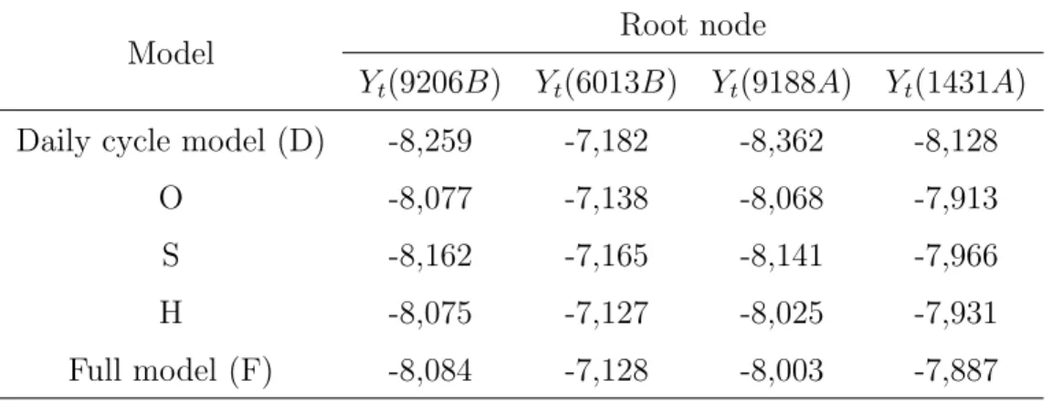
Table 2 gives the LPL for each of these models for all the root nodes. All the models with the daily cycle pattern and one single predictor variable (Models O, S and H) provide better forecasts than Model D, with Model H being the best one for almost all sites. When comparing these models with Model F, Models H and O provide slightly better forecasts for site 9206B and Model H also shows a marginal improvement over Model F for 6013B, whereas Model F is the best among all models for sites 9188A and 1431A. A model using Model D with the inverse of headway was also considered (since this variable can be viewed as the inverse of flow and that is also suggested by the scatterplots in Figure 3), but gave worse performance compared to model H.
Although Model F does not necessarily gives the best forecasts for all sites, as mentioned in Section 4.1, from a traffic modelling perspective it is sensible to retain all the variables in the model.
5.2
Children and grandchildren of the root nodes
In order to assess the effects of including predictor variables for root nodes and children, forecasts were obtained using LMDMs for the same four (separate) bivariate series that were considered in Table 1. For each bivariate series, three LMDMs were considered:
TABLE 3 ABOUT HERE
• Model F/D uses Model F for root node and Model D for child;
• Model F/F uses Model F for both root node and child.
To also evaluate the effect of considering parent flows when forecasting flows of children, independent DLMs using all predictor variables (for both parent and child) were also fitted for each of the bivariate series. The LPLs for all of these models are shown in Table 3.
From Table 3 it is clear that Model F/F is the best model among all possible alternatives for each bivariate series. What’s more, Model F/F provides better forecasts than independent DLMs using all predictor variables for each of the bivariate series. Thus, the inclusion of parent information in addition to the predictor variables when forecasting a child, is better than simply including the predictor variables.
Notice also that Model F/D provides better forecasts when compared to Model D/D for all bivariate series in Table 3. Thus, using the predictor variables in the LMDM seems to improve not only the forecasts at the same site that occupancy, headway and speed were measured, but also affects the quality of the forecasts of its descendants in the DAG.
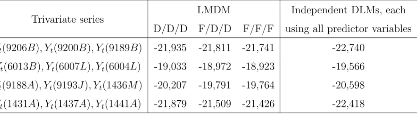
Similar conclusions can be made when looking at trivariate time series forecasts based on results from Table 4, which shows LPLs for LMDMs for series formed by root nodes together with one of their children and one of their associated grandchildren. In this case, model F/D/D, for example, means an LMDM for a trivariate time series using Model F for root node and Model D (with parents as regressors) for its child and grandchild.
TABLE 4 ABOUT HERE
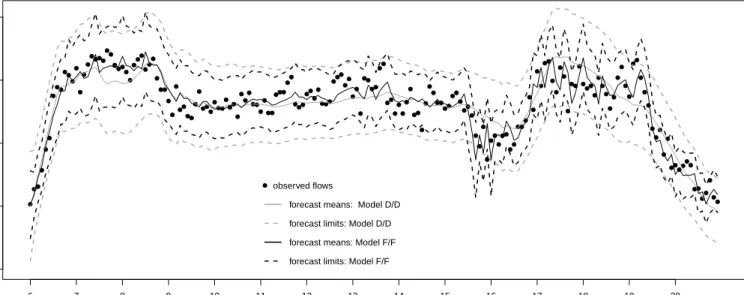
As another illustration of model improvement when considering occupancy, headway and speed for flow forecasting, Figure 4 shows the observed flows on a specific day for site 9200B,
together with forecast means and one-step ahead forecast limits (forecast mean±2×forecast
standard deviation). The forecasts were calculated considering LMDMs D/D and F/F for
the bivariate time series (Yt(9206B), Yt(9200B)). The F/F model has narrower forecast
limits than the D/D model for the whole day, which is an indication that the inclusion of the predictor variables in the model decreases the uncertainty about flows when compared to an LMDM modelling the daily cycle alone. Notice also that the F/F model captures
the deviations from the usual flow patterns that occur during the periods 07:30-08:30 and 15:00-17:00, providing much more accurate forecasts than the D/D model. These periods correspond to peak times in the network, times when in fact flow forecasting models are most useful.
In Figure 4, most observations lie within their respective forecast limits. This should happen for approximately only 95% of observations in a well-calibrated model. Over the whole forecast period, both daily cycle (D) and full (F) models are well-calibrated for the root nodes with roughly 95% of observations lying within the forecast limits for each series. When forecasting child variables as well, however, Model D/D overestimates the forecast uncertainty with roughly 99% to 100% of observations falling within the forecast limits for each series, while this time model F/F is well-calibrated with a coverage of roughly 95%. A similar behaviour was observed for models D/D/D and F/F/F when including grandchild variables. This suggests that, for child and grandchild variables, there are factors affecting the flow variation that are captured by the inclusion of extra variables as predictors in the model.
FIGURE 4 ABOUT HERE
6
Final remarks
The methodology proposed in this paper tackles both the problem of using extra traffic variables for enhancing flow forecasts, whilst also accommodating, and taking advantage of, the multivariate nature of the problem to provide real-time multivariate flow forecasts. Neither of these issues are often considered in traffic modelling.
The performance of all models presented here was based on past traffic data. However, when using the LMDM in an on-line environment in practice, on-line model monitoring would be crucial in order to monitor how well the model is performing over time, as well as to identify when model intervention is required (the technique of intervention allows information regarding a change in the time series to be fed in the model to maintain forecast performance — see Queen and Albers, 2009). Given that the LMDM is a set of (conditional) DLMs, it should be relatively straightforward to adapt established monitoring and intervention techniques for DLMs (as described in West and Harrison, 1997) into the LMDM context.
References
Abdulhai, B., Porwal, H. and Recker, W. (1999). Short-term Freeway Traffic Flow Prediction Using Genetically-optimized Time-delay-based Neural Networks. In: Proceedings of the 78th Annual Meeting of the Transportation Research Board. National Academies Press, Washington, DC.
Ahmed, M. S. and Cook, A. R. (1979). Analysis of freeway traffic time-series data by using Box-Jenkins techniques,Transportation Research Record,773, 47-49.
Anacleto, O., Queen, C.M. and Albers, C.J. (2013). Multivariate forecasting of road traffic flows in the presence of heteroscedasticity and measurement errors. Applied Statistics,62, Part 2. Ashton, W.D. (1966). Theory of Road Traffic Flow. Methuen’s Monographs on Applied Prob-ability and Statistics. John Wiley, London.
Chandra, S.R. and Al-Deek, H. (2009). Predictions of Freeway Traffic Speeds and Volumes Using Vector Autoregressive ModelsJournal of Intelligent Transportation Systems,13, 53-72.
Clark, S. (2003). Traffic prediction using multivariate non-parametric regression. Journal of Transportation Engineering,129(2), 161-168.
Gilmore, J.F., and Abe, N. (1995). Neural network models for traffic control and congestion prediction. Journal of Intelligent Transportation Systems,3, 231-252.
Greenshields, B.D (1935). A study of traffic capacity. Highway Research Board Proceedings,
14, 448-474.
Harrell, F.E. (2001). Regression modelling strategies with applications to linear models, logistic regression and survival analysis. Springer-Verlag, New York.
Hastie, T., Tibshirani, R., and Friedman, J. (2001). The Elements of Statistical Learning. Springer-Verlag, New York.
Innamaa, S. (2000). Short-term prediction of traffic situation using MLP-neural networks,in: Proceedings of the 7th World Congress on Intelligent Transportation Systems, Turin, Italy.
Kamarianakis, Y., and Prastacos, P. (2005). Space-time Modeling of Traffic Flow. Computers & Geosciences,31, 119-133.
Levin, M. and Tsao, Y.D. (1980). On forecasting freeway occupancies and volumes.Transportation Research Record,773, 47-49.
Li, B. (2009). A Non-Gaussian Kalman Filter With Application to the Estimation of Vehicular Speed. Technometrics,51, 162-172.
Petris, G., Petrone, S. and Campagnoli, P. (2009). Dynamic Linear Models With R. Springer, New York.
Prado, R., and West, M. (2010). Time Series: modelling, Computation and Inference. Chap-man & Hall, New York.
Queen, C.M. and Smith, J.Q. (1993). Multiregression dynamic models. Journal of the Royal Statistical Society, B,55(4), 849-870.
Queen, C.M., Wright, B.J. and Albers, C.J. (2007). Eliciting a Directed Acyclic Graph for a Multivariate Time Series of Vehicle Counts in a Traffic Network. Australian and New Zealand Journal of Statistics,49(3), 221-239.
Queen, C.M., Wright, B.J. and Albers, C.J. (2008). Forecast covariances in the linear multire-gression dynamic model. Journal of Forecasting,27, 175-191.
Queen, C.M. and Albers, C.J. (2009). Intervention and Causality: Forecasting Traffic Flows Using a Dynamic Bayesian Network. Journal of the American Statistical Association,104, 669-681. Stathopoulos, A. and Karlaftis, G.M. (2003). A multivariate state space approach for urban traffic flow modelling and prediction. Transportation Research Part C,11(2), 121-135.
Sun, S. L., Zhang, C. S., and Yu, G. Q. (2006). A Bayesian Network Approach to Traffic Flows Forecasting.IEEE Transactions on Intelligent Transportation Systems.,7, 124-132.
Tebaldi, C., West, M. and Karr, A.K. (2002). Statistical analyses of freeway traffic flows.
Journal of Forecasting,21, 39-68.
Vlahogianni, E. I., Golias, J. C. and Karlaftis, M. G. (2004). Short-term traffic forecasting: Overview of objectives and methods. Transport Reviews,24(5), 533-557.
West, M. and Harrison, P.J. (1997). Bayesian Forecasting and Dynamic Models (2nd edition) Springer-Verlag, New York.
Whittaker, J., Garside, S. and Lindveld, K. (1997). Tracking and predicting a network traffic process. International Journal of Forecasting,13, 51-61.
Table 1: LPLs for LMDMs with different seasonal representations. LMDM
Bivariate series seasonal factors static splines dynamic splines
Yt(9206B), Yt(9200B) -8,794 -8,857 -8,570
Yt(6013B), Yt(6007L) -8,159 -8,157 -7,886
Yt(9188A), Yt(9193J) -8,581 -8,647 -8,336
Yt(1431A), Yt(1437A) -9,056 -8,839 -8,597
Table 2: LPLs for various models for all root nodes of the Manchester network.
Model Root node
Yt(9206B) Yt(6013B) Yt(9188A) Yt(1431A)
Daily cycle model (D) -8,259 -7,182 -8,362 -8,128
O -8,077 -7,138 -8,068 -7,913
S -8,162 -7,165 -8,141 -7,966
H -8,075 -7,127 -8,025 -7,931
Full model (F) -8,084 -7,128 -8,003 -7,887
Table 3: LPLs for different LMDMs for bivariate time series from the Manchester network.
Bivariate series LMDM Independent DLMs, each
D/D F/D F/F using all predictor variables
Yt(9206B), Yt(9200B) -15,156 -15,064 -14,986 -15,467
Yt(6013B), Yt(6007L) -13,620 -13,559 -13,520 -13,852
Yt(9188A), Yt(9193J) -14,591 -14,219 -14,208 -14,517
Table 4: LPLs for different LMDMs for trivariate time series from the Manchester network
Trivariate series LMDM Independent DLMs, each
D/D/D F/D/D F/F/F using all predictor variables
Yt(9206B), Yt(9200B), Yt(9189B) -21,935 -21,811 -21,741 -22,740
Yt(6013B), Yt(6007L), Yt(6004L) -19,033 -18,972 -18,923 -19,566
Yt(9188A), Yt(9193J), Yt(1436M) -20,207 -19,791 -19,764 -20,598
(a) (b) 9206B 9200B 1445B 6012A 6007A 6006K 1441A 9199A 9197M 9205A 1431A 6002A 1437A 1438B 6013B 6002B 6007L 9194K 6004L Z 9192M 9190L 9188A 9189B 9195A 9193J 6003K 1436M 1429B 1436B M62 M602 M60 M60 0 100 300 500 700 flo w
Mon Tue Wed Thu Fri
Figure 1: (a) Schematic diagram of the Manchester network. (b) 5-minute flows for site 9206B (black line) and 1437A (grey line) for 4–8 October 2010.
Yt(9206B) Yt(9188A) Yt(1437A) Yt(6013B) Yt(9200B) Yt(1445B) Yt(9189B) Yt(Z) Yt(1438B) Yt(6006K) Yt(1431A) Yt(1441A) Yt(9197M) Yt(6002A) Yt(9199A) Yt(9205A) Yt(9193J) Yt(9195A) Yt(6003K) Yt(1436M) Yt(1436B) Yt(1429B) Yt(6012A) Yt(6007A) Yt(6002B) Yt(6007L) Yt(9194K) Yt(6004L) Yt(9192M) Yt(9190L)