Konstantin A. Kholodilin*
Forecasting the Turns of German Business Cycle:
Dynamic Bi-Factor Model with Markov Switching
Discussion Papers
Berlin, Juni 2005
IMPRESSUM © DIW Berlin, 2005 DIW Berlin
Deutsches Institut für Wirtschaftsforschung Königin-Luise-Str. 5
14195 Berlin
Tel. +49 (30) 897 89-0 Fax +49 (30) 897 89-200 www.diw.de
ISSN print edition 1433-0210 ISSN electronic edition 1619-4535
All rights reserved.
Reproduction and distribution in any form, also in parts, requires the express written permission of DIW Berlin.
Forecasting the Turns of German Business Cycle:
Dynamic Bi-Factor Model with Markov Switching
Konstantin A. Kholodilin
∗June 16, 2005
Abstract
In this paper a dynamic bi-factor model with Markov switching is pro-posed to measure and predict turning points of the German business cycle. It estimates simultaneously the composite leading indicator (CLI) and composite coincident indicator (CCI) together with corre-sponding probabilities of being in recession. According to the bi-factor model, on average, CLI leads CCI by 3 months at both peaks and troughs. The model-derived recession probabilities of CCI and those of CLI with a lag of 2–3 months capture the turning points of the ECRI’s and OECD’s reference cycle much better than the dynamic single-factor model with Markov switching.
Keywords: Forecasting turning points; composite coincident indi-cator; composite leading indiindi-cator; dynamic bi-factor model; Markov-switching
JEL classification: E32; C10
∗DIW Berlin, [email protected]
List of Tables K. A. Kholodilin
Contents
1 Introduction 1
2 Model 2
3 Estimation and evaluation 8
3.1 Estimation . . . 8 3.2 Evaluation . . . 11 4 Summary 15 References 15 Appendix 19
List of Tables
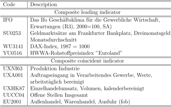
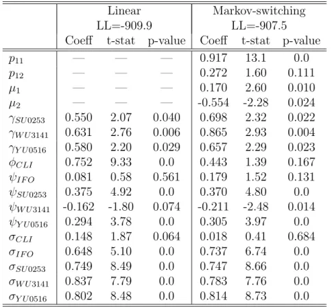
1 Component series of German CLI and CCI, monthly data 1991:1–2005:3 . . . 19 2 Estimates of the parameters of German single-factor linear and
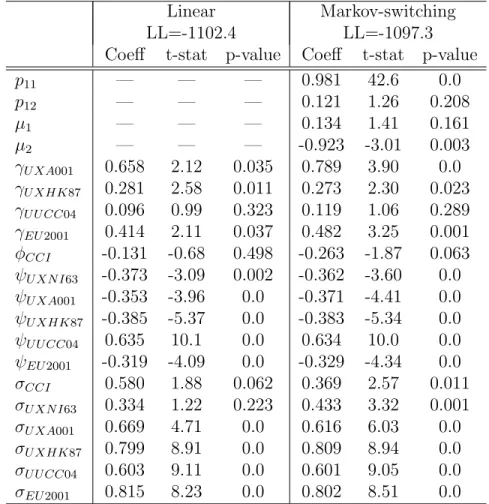
Markov-switching model of CLI, monthly data 1991:1–2005:3 20 3 Estimates of the parameters of German single-factor linear and
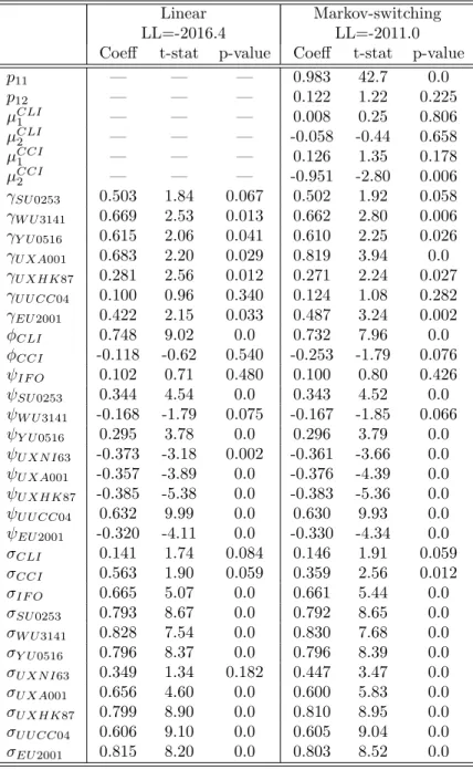
Markov-switching model of CCI, monthly data 1991:1–2005:3 21 4 Estimates of the parameters of German bi-factor Markov-switching
model (a), monthly data 1991:1–2005:3 . . . 22 5 Estimates of the parameters of German bi-factor Markov-switching
model (c), monthly data 1991:1–2005:3 . . . 23 6 Official and model-derived chronologies of German business
cycle, monthly data 1991:2–2005:3 . . . 24 7 The in-sample predicting performance of the dynamic factor
models with Markov switching (measured by the Quadratic Probability Score), monthly data 1991:2–2005:3 . . . 25
1 Introduction K. A. Kholodilin
1
Introduction
Burns and Mitchell (1946) defined business cycles as recurrent sequences of cumulative expansions and contractions diffused over a multitude of economic processes. Diebold and Rudebusch (1996) later summarized these classical cycles into two key features: co-movements among many macroeconomic in-dicators and asymmetry between the cyclical phases.
The first feature allows constructing the composite leading indicator (CLI) and composite coincident indicator (CCI) in order to measure and predict the state of affairs. CLI is used mostly to forecast the changes in CCI, since by its very nature the CLI is leading the CCI and hence the business cycle. The CCI is contemporaneous with the current state of the economy and can be considered as a proxy of the real GDP.
Both features can be jointly analyzed within a single model thanks to the contributions of Stock and Watson (1991), who re-introduced the dynamic factor model in the econometric research, and Hamilton (1989), who pro-posed a model with Markov-switching dynamics. The resulting dynamic single-factor model with Markov switching was suggested by Kim (1994) and Kim and Yoo (1995) and implemented for the first time by Chauvet (1998). It permits simultaneously capturing the co-movement and the cyclical asym-metry. This model has become already quite a standard tool of analyzing the business cycle. It has been successfully applied to the U.S. data by Chauvet (1998) and Kim and Nelson (1999), to the data of several European economies by Kaufmann (2000), to the Brazilian data by Chauvet (2002), to the Japanese data by Watanabe (2003), and to the Polish and Hungarian data by Bandholz (2005). In Germany the first such a model (although with only two component series, which raises a question of its identifiability) was estimated by Bandholz and Funke (2003).
The first attempt, as far as we know, to build a dynamic bi-factor model with Markov switching, in which the CLI and CCI are estimated simultane-ously, was undertaken in Kholodilin (2001) and Kholodilin and Yao (2005). Using this model the turning points can be measured and predicted simul-taneously and in a more timely manner. Kholodilin (2001) and Kholodilin and Yao (2005) applied the model to the U.S. data, whereas this paper con-centrates on the German data.
2 Model K. A. Kholodilin
The paper is structured as follows. In section 2 a dynamic bi-factor model with Markov-switching is set up. Section 3 estimates the model using the maximum likelihood method based on four leading indicators and five co-incident indicators for the German economy. In section 4 the results are evaluated in sample. The last section concludes the paper.
2
Model
Basically, the dynamic factor model decomposes the dynamics of a group of observed time series into two unobserved sources of fluctuations: (1) the common factor or factors, which are common to all the component series or to the particular subgroups of them; (2) the specific, or idiosyncratic, factors — one per each observed series. In fact, the specific factors ”explain” the remaining variation, which is left after the common factors were extracted. The non-linear dynamic factor models, e.g. the model with Markov switching or with smooth transition autoregressive dynamics (see Kholodilin (2002)), in addition, take into account the possible asymmetries arising in the differ-ent states, or regimes. Here by the state we mean the phases of business cycle. Moreover, the parametric dynamic factor models explicitly specify the dy-namics of the latent (unobserved) factors. In the model examined in this paper both common and specific factors are modelled as autoregressive (AR) processes.
In the dynamic bi-factor model the set of the n observed variables is split in two disjoint subsets: nCLI leading andnCCI coincident indicators. The
com-mon dynamics of the time series belonging to each group are explained by a single common factor: CLI for the first group and CCI for the second group. Thus, the complete dynamic bi-factor model with Markov switching can be written as a system of the three equations, where the first equation decom-poses the observed dynamics into a sum of common and idiosyncratic factors and the last two equations specify the ”law of motion” of the latent common and specific factors.
2 Model K. A. Kholodilin
The decomposition of the observed dynamics:
µ ∆yCLI t ∆yCCI t ¶ = µ ΓCLI OnCLI OnCCI ΓCCI ¶ µ ∆fCLI t ∆fCCI t ¶ + µ uCLI t uCCI t ¶ (1)
The dynamics of common factors:
µ ∆fCLI t ∆fCCI t ¶ = µ µCLI(sCLI t ) µCCI(sCCI t ) ¶ + µ φ1.11 φ1.12 φ1.21 φ1.22 ¶ µ ∆fCLI t−1 ∆fCCI t−1 ¶ + . . .+ µ φl.11 φl.12 φl.21 φl.22 ¶ µ ∆fCLI t−l ∆fCCI t−l ¶ + µ εCLI t εCCI t ¶ (2)
The dynamics of idiosyncratic factors:
µ uCLI t uCCI t ¶ = µ ΨCLI 1 OnCLI×nCCI OnCCI×nCLI Ψ CCI 1 ¶ µ uCLI t−1 uCCI t−1 ¶ + . . .+ µ ΨCLI m OnCLI×nCCI OnCCI×nCLI ΨCCIm
¶ µ uCLI t−l uCCI t−l ¶ + µ ηCLI t ηCCI t ¶ (3) where ∆yCLI
t and ∆ytCCI are the nCLI ×1 and nCCI ×1 vectors of the
ob-served leading and coincident variables in the first differences; ∆fCLI t and
∆fCCI
t are the latent common factors in the first differences; uCLIt and uCCIt
are the nCLI×1 and nCCI×1 vectors of the latent specific factors;εCLIt and
εCCI
t are the disturbances of the common factors, whereas ηCLIt and ηtCCI
are the nCLI×1 andnCCI ×1 vectors of disturbances of the specific factors.
ΓCLI and ΓCCI are the nCLI ×1 and nCCI ×1 factor loadings vectors
link-ing the observed series to the common factors. µCLI(sCLI
t ) and µCCI(sCCIt )
are the state-dependent intercepts of CLI and CCI. φi are the
autoregres-sive coefficients of common factors; and ΨCLI
i and ΨCCIi are the matrices of
the autoregressive coefficients of the idiosyncratic factors. On and On×m are
n×1 vector and n×m matrix of zeros, correspondingly. Finally, sCLI t and
sCCI
t are the unobserved state variables following a first-order Markov chain
2 Model K. A. Kholodilin characteristic element is pij = prob(st =j|st−1 =i), that is, the probability
of being today in regime j given that yesterday’s regime was i.
In the two-regime (expansion-recession, or high-low growth rate) case a state variable st takes two values: 0 or 1. Depending on the regime, the common
factor’s intercept assumes different values: low in contractions and high in expansions. Thus, the common factors grow faster during the upswings and slower (or even decline) during the downswings of the economy.
The dynamic bi-factor model with Markov switching described above is based on the following assumptions:
• The common factors’ disturbances, εt = (εtCLI|εCCIt )0, and the specific
factors’ disturbances, ηt = (ηtCLI|ηtCCI)0, are mutually and serially
un-correlated: µ εt ηt ¶ ∼NID µµ 0 0 ¶ , µ Σ(st) O2×n On×2 Ω ¶¶ (4) where Σ(st) is the diagonal 2 × 2 variance-covariance matrix of common
factors, with the common factor residual variances on the main diagonal,
σ2
CLI(st) and σCCI2 (st), which may be state dependent; Ω is the diagonal
n×n variance-covariance matrix of the idiosyncratic disturbances.
• There is no Granger causality between the common factors: φi.12 =φi.21
∀i ∈[1, l]. This is a bit strong restriction. Together with the previous assumption it implies that the only way the CLI is linked to the CCI is through the intercept, when the state variables of both common factors are interdependent. There can also exist a relationship between the volatilities of two common factors when their residual variances are state dependent and their state variables are related. In principle, this assumption can be relaxed without changing much the outcomes of the model. Here it is used only for the sake of parsimony.
• This assumption specifies the state variable dynamics. In fact, we can consider three cases:
(a) there is a single state variable, st, such that sCLIt = sCCIt , in
other words, the non-linear dynamics of the common factors are identical;
2 Model K. A. Kholodilin (b) sCLI
t and sCCIt are completely independent;
(c) sCLI
t and sCCIt are neither identical as in (a) nor independent as
in (b) but interdependent.
Now let us consider in more detail the specification of the Markov switching in the non-linear dynamic bi-factor model under inspection. In the case (a) above there is only one state variable and it all boils down to the standard two-regime Markov switching model as in Hamilton (1989). The transition probabilities matrix then looks like:
π = µ p11 1−p11 1−p22 p22 ¶ (5) In the cases (b) and (c) there are two state variables: one per each common factor. This means that each composite indicator has its own recessions and expansions. Therefore to describe the whole process, a compound state variable, comprising both sCLI
t and sCCIt , should be constructed as it is done
in Phillips (1991). This compound variable will have four different states: Composite st= 1 st = 2 st= 3 st= 4
Leading sCLI
t = 1 sCLIt = 2 sCLIt = 1 sCLIt = 2
↑ ↓ ↑ ↓
Coincident sCCI
t = 1 sCCIt = 1 sCCIt = 2 sCCIt = 2
↑ ↑ ↓ ↓
where the arrows show whether the economy goes up (expansion) or down (recession).
The dimension of the transition probabilities matrix is then 4×4 and its structure depends on which of the cases is assumed: (b) or (c). In the case (b), when both state variables are independent, the transition probabilities matrix of the compound state variable is a Kronecker product of the transi-tion probabilities matrices of the individual state variables: π =πCLI⊗πCCI.
This is equivalent to:
π= pCLI
11 pCCI11 (1−pCLI11 )pCCI11 pCLI11 (1−pCCI11 ) (1−pCLI11 )(1−pCCI11 )
(1−pCLI
22 )pCCI11 pCLI22 pCCI11 (1−p22CLI)(1−pCCI11 ) pCLI22 (1−pCCI11 )
pCLI
11 (1−pCCI22 ) (1−pCLI11 )(1−p22CCI) pCLI11 pCCI22 (1−pCLI11 )pCCI22
(1−pCLI
22 )(1−pCCI22 ) pCLI22 (1−pCCI22 ) (1−pCLI22 )pCCI22 pCLI22 pCCI22
2 Model K. A. Kholodilin Under the hypothesis (c) the two individual state variables are assumed to be interrelated in the sense that the CLI is supposed to enter the recessions (expansions) several periods earlier than the CCI. This is a kind of inter-mediate case between completely independent and identical state variables corresponding to CLI and CCI.
As Phillips (1991) remarks, the model with an integer lag exceeding one period would require a Markov process with the order higher than 1. How-ever, the real-valued (positive) lag can be modelled with a first-order Markov process by constructing the following transition probabilities matrix:
π= p11 1−p11 0 0 0 1− 1 A 0 A1 1 B 0 1− B1 0 0 0 1−p22 p22 (7)
where A and B are the expected leads in the recession and expansion, cor-respondingly. The expected lead of CLI with respect to CCI when entering the low-growth regime (st= 2) is:
A = 1 +p(st= 2|st−1 = 2) +p(st= 2|st−1 = 2)2+. . . (8)
that is
A= 1
1−p(st= 2|st−1 = 2)
(9) We are going to examine three models corresponding to the three above stated cases. By comparing these models one can test the underlying hy-potheses. Model (c) is an unrestricted version of model (a). Thus, by im-posing restrictions on the parameters A and B one can test the hypothesis of identical versus interdependent with lead non-linear cyclical dynamics, for example, using the Likelihood-Ratio test. The null of identical state variable implies that A = B = 1. The formal testing of (a) versus (b) or (c) versus (b) is a more complicated enterprise. Under the null of identical or interde-pendent state variable the second state variable is not identified. It means that we are confronting the famous nuisance parameter problem similar, for instance, to testing the hypothesis of two regimes versus three regimes.
2 Model K. A. Kholodilin In order to estimate the above dynamic factor models with Markov switching, they are expressed in the state-space form:
∆yt=Axt (10)
xt=α(st) +Cxt−1+vt (11)
wherext= (ft|ut)0 is the state vector containing stacked on top of each other
the vector of common factors and the vector of specific factors; vt is the
vector of the common and idiosyncratic factors’ disturbances with mean zero and variance-covariance matrix Q; α(st) = (µCLI(st), µCCI(st), ...,0)0 is the
state-dependent vector of intercepts. The structure of the system matrix A
is defined as in Kholodilin (2001), while matrix C has somewhat different structure given the fact that the assumption of Granger causality between the common factors has been removed from this model:
C = ΦCLI O 0 O ΦCCI Ψ1 . .. 0 Ψn (12)
where matrices ΦCLI, ΦCCI, and Ψi (i= 1, ..., n) are formulated exactly the
same way as in Kholodilin (2001).
There are different ways of estimating the unknown parameters and the la-tent factors (maximum likelihood, EM, MCMC techniques — see Kim and Nelson (1999) for more details). Here we applied the maximum likelihood method with log-likelihood function obtained using Kalman filter recursions. To save space we will not present them here, referring the reader, for instance, to Hamilton (1994) who gives a very clear and systematic explanation of the Kalman filter methodology.
Note that in the case (b) two separate dynamic single-factor models for CLI and CCI can be estimated, instead of a rather cumbersome bi-factor model.
3 Estimation and evaluation K. A. Kholodilin
3
Estimation and evaluation
3.1
Estimation
The component series of both CLI and CCI were picked up from a dataset of 147 series representing various sectors of German economy and available at the site of Deutsche Bundesbank in the Internet. The selection criterion was the cross-correlations between the growth rates of these series. The following selection procedure was employed.
First, the coincident series were selected. We assumed that the industrial production is a natural proxy of the monthly composite coincident indicator. Hence as component series of CCI were chosen those variables, for which the cross-correlation with UXNI63 achieves its maximum at zero lag and is the highest compared to the remaining series. Surprisingly the new orders series, which is normally thought to be a leading indicator, turned out to be rather coincident one. This finding contradicts, e.g., the conclusions of Fritsche and Kuzin (2005). However, in the cited article the leading nature of the indicators is determined with respect to a particular reference chronol-ogy series and so the conclusions depend on the choice of such a chronolchronol-ogy. On the other hand, the evidence of the leading nature of new orders is not very strong. On the other hand, the cross-correlation analysis conducted in Fritsche and Stephan (2000) leads to the same conclusion as ours about the coincident nature of the new orders in manufacturing. The components of CLI are leading the industrial production and CCI and are highly but not too much correlated among themselves. It is important to avoid collinearity of the components and at the same time to guarantee their high enough cor-relation, which is indispensable for the extraction of the common factor. The data employed in this study are four leading indicators and five co-incident indicators. They are shortly described in Table 1 of Appendix. The component series of CLI are: Ifo expectations indicator (IFO), 12-month interest rate at Frankfurt’s money market (SU0253), DAX stock exchange index (WU3141), and HWWA-index of raw materials’ prices ”Euroland” (YU0516). The components of CCI are: the index of industrial production (UXNI63), new orders in manufacturing (UXA001), retail trade (UXHK87), job vacancies (UUCC04), and exports of goods in FOB prices (EU2001). UUCC04 is a broad measure of the labor input of the overall economy. The
3 Estimation and evaluation K. A. Kholodilin remaining four indicators represent three major sectors of German economy: manufacturing (UXNI63 and UXA001), trade (UXHK87), and foreign trade (EU2001), which is especially important for Germany. Together, according to the German national accounting of 2004, the industrial production and internal trade account for about 43% of the German GDP, while the exports represent 37% of the GDP.
All the series are tested for unit roots using the augmented Dickey-Fuller test. Each series is tested for random walk with drift and deterministic trend, random walk with drift, and random walk only. It turns out that all the series have unit root. All the series are also tested for cointegration. The cointegration between the leading as well as between the coincident series was detected. As in Stock and Watson (1991) and Kim and Nelson (1999), the first differences of the logarithms of the original time series are taken and then demeaned and standardized.
We estimated three dynamic bi-factor models with Markov-switching cor-responding to the hypotheses (a), (b), and (c) mentioned in the previous section. Recall that these hypotheses are defined by the following equations: (a) Hypothesis of identical Markov-switching dynamics of CLI and CCI — equations (1) – (4) and (5). The model, in which CLI and CCI enter the recessions and expansions simultaneously, without any leads. (b) Hypothesis of independent Markov-switching dynamics of CLI and CCI
— equations (1) – (4) and (6). This model can be alternatively esti-mated as two separate dynamic single-factor models with two-regime switching based on coincident and leading indicators correspondingly. Each of the separate dynamic single-factor models is identical to that of Chauvet (1998) and Kim and Nelson (1998).
(c) Hypothesis of interdependent Markov-switching dynamics of CLI and CCI — equations (1) – (4) and (7). A dynamic bi-factor model with interdependent cyclical dynamics that results in four-regime switching: two regimes for the leading indicator and two regimes for the coincident indicator. The composite leading factor (or CLI) switches between its regimes earlier than the composite coincident indicator (or CCI). We determined the lag structure by balancing two requirements: on the one hand, our composite indicators should have some dynamics, that is, the lag
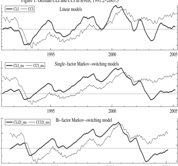
3 Estimation and evaluation K. A. Kholodilin order must be higher than zero; on the other hand, due to the short sample the lag order cannot be too high. Therefore both the common and idiosyn-cratic factors are specified as AR(1). For the identification purposes, the first loading factor in all the models is normalized to 1, i.e. the loading factor of IFO for leading indicators and that of UXNI63 for coincident indicators. The parameter estimates and their standard errors corresponding to single-factor models of CLI and CCI and to bi-single-factor models are reported in Tables 2 through 5. The parameters of linear and Markov-switching models are reported. Both MS models of composite leading and coincident indicators clearly distinguish between two regimes of positive and negative growth rates. ∆CLIhas a high positive autoregressive coefficient varying for different mod-els in the interval between 0.462 and 0.752, whereas ∆CCI has a negative, not always significant autoregressive coefficient varying between -0.228 and -0.113. Correspondingly, as one can see on Figure 1, the CLI’s profile is much smoother than that of CCI.
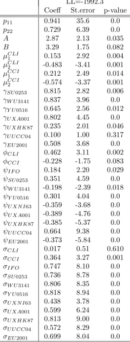
Factor loadings are positive and mostly significant, except for that of UUCC04. They are somewhat higher in the bi-factor model. The magnitudes of the factor loadings are roughly the same, which is an indirect indicator of the approximately equal weights of the components in both CLI and CCI. The estimates of the single- and bi-factor models, linear and Markov-switching models do not differ very much. The estimated lead-time of CLI over CCI, which can be estimated under the hypothesis (c), is approximately 3 for both peaks and troughs. For the CLI estimated as a single-factor model with Markov switching the transition probability of being today in expan-sion given that yesterday was expanexpan-sion, p11 = 0.917 is much higher than
the transition probability of being today in recession given that yesterday was recession, p22 = 1−p12 = 0.728, implying that the expected duration
of expansions is approximately equal to 12 months and is greater than the expected duration of recessions, which is equal to 4 months. These dura-tions are a little bit too small, especially the expected duration of recessions. The estimates of the dynamic single-factor model with Markov switching for CCI (see Table 3) suggest that the expected duration of CCI’s expan-sions is about 53 months and the expected duration of CCI’s recesexpan-sions is 8 months. The same durations result from the bi-factor model with Markov
3 Estimation and evaluation K. A. Kholodilin switching corresponding to the hypothesis (a) — see Table 4. In fact, the conditional recession probabilities obtained from this model almost coincide with those obtained from the single-factor model of CCI. Finally, according to the dynamic bi-factor model with Markov switching corresponding to the hypothesis (c) — Table 5 — the expected duration of expansions is 17 months (more than 5 quarters, or roughly 1.5 years) and the expected duration of recessions is about 4 months (1 quarter).
We can also test which of the three hypotheses fits the data best. At least this can be done for the models (a) and (c), where for the compar-ison the likelihood ratio test can be employed. According to the likeli-hood ratio test, with two degrees of freedom and the test statistic equal toLR = 37.3> LR0.01(2) = 9.21 the model (c) is significantly different from
the model (a), and hence the null of completely identical non-linear cyclical dynamics can be rejected in favor of CLI leading the CCI.
3.2
Evaluation
Unlike for the USA, we do not have any generally accepted business cycle chronology for Germany. Among the few available alternative chronologies1
we selected two, to which the recession probabilities of our non-linear models will be compared, namely: ECRI’s growth cycle dating2 and the OECD’s
dating. Both datings are reported in the first four columns of Table 6. The first chronology relies upon the growth rates. This dating seems to be more appropriate to the case of Germany than the so-called ECRI’s classical cycle chronology, because over the whole sample, 1991–2005, the absolute decline in level of GDP was a rather rare event, whereas the deceleration of the growth rates happens much more frequently and is an event, which is worth predicting.
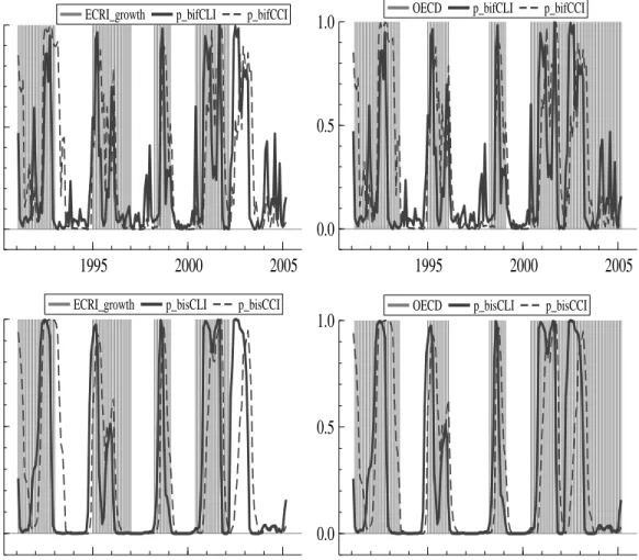
The profiles of CLI and CCI estimated from the dynamic single- and bi-factor models with and without Markov switching are plotted on Figure 1.
1We do not consider here the chronology obtained by Heilemann and M¨unch (1999),
since it ends in 1994, although their approach appears to be fruitful and can be applied in the future research for a sample covering more recent past.
2An important disadvantage of this chronology is that it was updated for the last time
3 Estimation and evaluation K. A. Kholodilin The filtered and smoothed conditional probabilities of recessions correspond-ing to these models are plotted in Figures 2 and 3 respectively. We do not display the conditional recession probabilities of the model (a), because they are almost identical to those of the single-factor model for CCI.
In the bi-factor models with interdependent non-linear dynamics (two state variables), there are four regimes: two for the common leading factor and the other two for the common coincident factor. In the former case, the CLI’s recession probabilities are obtained as the sum of the conditional probabili-ties of regimes 2 and 4 (”low leading factor and high coincident factor” and ”low leading factor and low coincident factor”), while CCI’s recession prob-abilities are the sum of the probprob-abilities of regimes 3 and 4. The recession probabilities stemming from the three models — (a), (b), and (c) — are very different. Whereas the conditional recession probabilities derived from the model (a) are almost identical with those corresponding to the single-factor model of CCI (model (b) estimated as two separate single-factor models), the estimated conditional probabilities derived from model (c) differ from those of model (a) and (b).
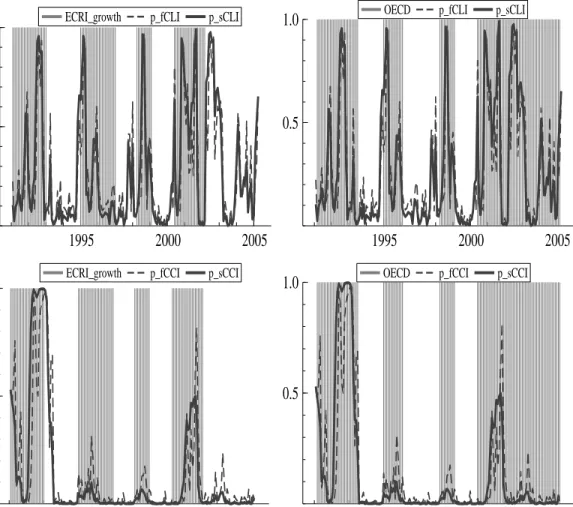
Under the hypothesis of completely independent cycles of CLI and CCI (model (b)), the conditional recession probabilities of CLI are quite volatile even after smoothing — see the upper panel of Figure 2. The shaded areas represent the recessionary phases of both official chronologies. The CLI’s recession probabilities signal five recessions, the first four of which roughly coincide with the ECRI’s growth cycle, whereas all the CLI’s recessions fall into the shaded areas of the OECD’s dating. The CCI’s conditional recession probabilities, plotted on the bottom panel of Figure 2, give only two signals of downswings: in 1992 and in 2001. The second signal is rather weak being lower than 0.5. The CCI’s probabilities are thus detecting a kind of classical cycle and not the growth cycle.
The situation changes drastically when model (c) — stating that the cyclical dynamics of CCI are lagging behind those of CLI — is estimated. As can be seen on Figure 3, the conditional recession probabilities of CLI underwent rather minor change. By contrast, the recession probabilities of CCI started resembling those of CLI with a clearly visible lag. Now both CLI and CCI signal five recessions.
3 Estimation and evaluation K. A. Kholodilin The dates of the two official reference chronologies can also be compared to the dates derived from the non-linear models considered in this paper — see Table 6. There the model-derived dates are obtained using the the algo-rithm of Chauvet and Piger (2003), which is applied here to the smoothed recession probabilities. Both the reference chronologies identify four reces-sions during the period under inspection. These recesreces-sions, save for the last one, are coinciding quite well. The recession probabilities of CLI and espe-cially of CCI derived from the model (c) have an improved concordance to the reference cycles compared to those derived from the model (b).
When the predicted reference chronology is known, the above comparison of the in-sample forecasting performance can be formalized using some criterion measuring the difference between the reference chronology and the model-derived dating. We use the Quadratic Probability Score (QPS) proposed in Brier (1950), which is based on probabilities derived from each model. Let Pt be the conditional probability that the economy is in recession,
esti-mated from the model; let Rt be the ECRI- or OECD-defined chronology (1
if recession, 0 otherwise), and the slightly modified version of QPS is given by: QP S = 1 T T X t=1 (Pt−τ −Rt) (13)
where τ is the time shift accounting for the possibly leading character of the recession probabilities andPt. QPS varies between 0 and 1, with a score of 0
corresponding to perfect accuracy. This is the unique proper scoring rule that is only a function of the discrepancy between realizations and model-derived probabilities (see Diebold and Rudebusch (1989) for further discussion). In order to compare the forecasting accuracy of different models; that is, to test whether the differences in the QPS of each model are significant, a test statistic developed by Diebold and Mariano (1995) was used. The null hypothesis states no difference between the predicted accuracy of the pair of models being compared. Given a sample path {dt}Tt=1 of a loss differential
series (Pt−τ −Rt in the above definition), we have √
T( ¯d−µ)−→d N(0,2πfbd(0)) (14)
where ¯d is the sample mean loss differential, fd(0) is the spectral density of
3 Estimation and evaluation K. A. Kholodilin Diebold-Mariano (DM) statistic for testing the H0 of equal forecast accuracy is defined as:
DM = q d¯
2πfbd(0)
T
(15) which is standardized and hence asymptotically distributed as N(0,1). The DM statistics are calculated with a rectangular window of length 15.
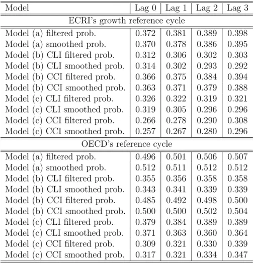
The in-sample predicting performance of the non-linear models estimated in this paper is reported in Table 7. It is measured by the QPS computed with respect to two above mentioned alternative reference chronologies. The in-sample performance is evaluated for different lags τ (see equation (13)) in order to account for the fact that CLI may lead the reference chronologies. In fact, the QPS is computed between the non-negative lags of the recession probabilities and binary reference datings.
The overall in-sample forecasting accuracy of all the examined models is far from being satisfactory — the QPS are very high. On average the model-derived chronologies correspond better to the ECRI’s growth cycle. This is mainly due to the differences in the reference chronologies in the last few years of the sample. It is the recession probabilities of CCI estimated in model (c) that are characterized by the best fit. According to the DM-statistics, which were computed but are not presented here to save the space, the chronolo-gies of CCI derived from the model (c) have significantly better in-sample forecasting accuracy than the chronologies of CCI derived from the model (b). This means that imposing condition of CLI’s cycle leading the CCI’s cycle, compared to the model where these two indicators are completely in-dependent, pays off. The minima of QPS for the CLI’s chronology derived from models (b) and (c) are achieved at lags 2 and 3, which perfectly corre-sponds to the estimates of the expected leads in recession and expansion. The performance of CLI is higher than that of model (a) and of CCI in model (b). Given the uncertainty about the reference chronology, the out-of-sample fore-casting exercise is hardly possible. Of course, we can make the forecasts with our models but their eventual performance will be affected both by the fore-casting errors and by the fact that it is not sure whether the selected reference chronologies reflect well the turning points of the German business cycle.
4 Summary K. A. Kholodilin
Finally, let us make a few remarks about the developments in the nearest future that can be inferred from the recession probabilities in the very end of the sample. Both from Figure 2 and 3 one can see that the conditional probability of getting into recession has increased in the last few months. This increase is especially pronounced in the probabilities derived from the single-factor model of CLI. It is, however, substantially less noticeable when the bi-factor model is considered. In any case the recession probabilities never exceed 0.5. Therefore for the moment we may expect an outbreak of recession soon or it can well be just a false alarm. To confirm or reject the signal a few more observations are needed.
4
Summary
The paper estimates a dynamic bi-factor model with Markov-switching based on four selected leading indicators and five coincident indicators of the Ger-man economy. This enables us to measure and predict the turning points of CLI and CCI simultaneously. Three alternative hypotheses were exam-ined: (a) switches between the recessionary and expansionary phases of CLI and CCI are identical; (b) these switches happen independently; and (c) the switches of the CLI precede those of CCI with some positive lead. In the latter case the model estimates the expected lead time of CLI over CCI as approximately 3 months at both peaks and troughs. The turning point dates derived from bi-factor models based on coincident indicators have a corre-spondence with ECRI- and OECD-defined recessions.
The test of in-sample performance of single-factor and bi-factor models rel-ative to ECRI- and OECD-defined turning points is conducted using the modified quadratic probability score and DM test statistics. CCI in model (c) has the lowest QPS and hence the highest conformity to the reference chronologies. Since CLIs lead the reference cycles, they have a high QPS and low conformity with the ECRI’s and OECD’s recessions at zero lag. The estimated CLIs have the closest match with the latter when they are moved 2–3 months forward. Therefore, this suggests that the estimated CLI and its probability of recession can be used as a predictor of the reference dates with an average lead of 3 months.
References K. A. Kholodilin
References
Bandholz, H. (2005). New composite leading indicators for Hungary and Poland. Ifo Working Paper No. 3.
Bandholz, H. and M. Funke (2003). In search of leading indicators of eco-nomic activity in Germany. Journal of Forecasting 22, 277–297.
Brier, G. (1950). Verification of forecasts expressed in terms of probability.
Monthly Weather Review 78, 1–3.
Burns, A. and W. Mitchell (1946). Measuring Business Cycles. New York. Chauvet, M. (1998). An econometric characterization of business cycle
dy-namics with factor structure and regime switching.International Economic Review 39, 969–996.
Chauvet, M. (2002). The Brazilian business and growth cycles. Revista Brasileira de Economia 56(1).
Chauvet, M. and J. M. Piger (2003). Identifying business cycle turning points in real time. Review (Federal Reserve Bank of St. Louis) (March), 47–61. Diebold, F. X. and R. S. Mariano (1995). Comparing predictive accuracy.
Journal of Business and Economic Statistics 13(3), 253–263.
Diebold, F. X. and G. D. Rudebusch (1989). Scoring the leading indicators.
Journal of Business 62, 369–402.
Diebold, F. X. and G. D. Rudebusch (1996). Measuring business cycles: A modern perspective. The Review of Economics and Statistics 78, 67–77. Fritsche, U. and V. Kuzin (2005). Prediction of business cycle turning points
in Germany. Jahrb¨ucher f¨ur National¨okonomie und Statistik 225/1, 23–43. Fritsche, U. and S. Stephan (2000). Leading indicators of German business
cycles: An assessment of properties. DIW Discussion Paper (207).
Hamilton, J. D. (1989). A new approach to the economic analysis of nonsta-tionary time series and the business cycle. Econometrica 57(2), 357–84. Hamilton, J. D. (1994). Time Series Analysis. New Jersey: Princeton
References K. A. Kholodilin Heilemann, U. and H. J. M¨unch (1999). Classification of the West German business cycles 1955-1994. Jahrb¨ucher f¨ur National¨okonomie und Statis-tik 219/5, 632–656.
Kaufmann, S. (2000). Measuring business cycles with a dynamic Markov switching factor model: An assessment using Bayesian simulation methods.
Econometrics Journal 3, 39–65.
Kholodilin, K. A. (2001). Latent leading and coincident factors model with Markov-switching dynamics. Economics Bulletin 3(7), 1–13.
Kholodilin, K. A. (2002). Two alternative approaches to modelling the non-linear dynamics of the composite economic indicator. Economics Bul-letin 3(26), 1–18.
Kholodilin, K. A. and V. W. Yao (2005). Measuring and predicting turning points using a dynamic bi-factor model. International Journal of Forecast-ing. forthcoming.
Kim, C.-J. (1994)). Dynamic linear models with Markov-switching. Journal of Econometrics 60, 1–22.
Kim, C.-J. and C. R. Nelson (1998). Business cycle turning points, a new coincident index, and tests of duration dependence based on a dynamic factor model with regime switching. The Review of Economics and Statis-tics 80(2), 188–201.
Kim, C.-J. and C. R. Nelson (1999). State-Space Models with Regime Switch-ing: Classical and Gibbs-Sampling Approaches with Applications. Cam-bridge: MIT Press.
Kim, M.-J. and J.-S. Yoo (1995). New index of coincident indicators: A mul-tivariate Markov switching factor model approach. Journal of Monetary Economics 36, 607–630.
Phillips, K. L. (1991). A two-country model of stochastic output with changes in regime. Journal of International Economics 31, 121–142.
Stock, J. H. and M. W. Watson (1991). A probability model of the coincident economic indicators. In L. K. and M. G. (Eds.), Leading Economic Indi-cators: New Approaches and Forecasting Records. Cambridge University Press.
References K. A. Kholodilin Watanabe, T. (2003). Measuring business cycle turning points in Japan with a dynamic Markov switching factor model. Monetary and Economic Studies 21 (1).
Appendix K. A. Kholodilin
Appendix
Table 1: Component series of German CLI and CCI, monthly data 1991:1–2005:3
Code Description
Composite leading indicator
IFO Das Ifo Gesch¨aftsklima f¨ur die Gewerbliche Wirtschaft, Erwartungen (R3), 2000=100, SA)
SU0253 Geldmarkts¨atze am Frankfurter Bankplatz, Dreimonatsgeld, Monatsdurchschnitt
WU3141 DAX-Index, 1987 = 1000
YU0516 HWWA-Rohstoffpreisindex ”Euroland” Composite coincident indicator UXNI63 Produktion Industrie
UXA001 Auftragseingang in Verarbeitendes Gewerbe, Werte, arbeitst¨aglich bereinigt
UXHK87 Einzelhandelumsatz, Volumen, kalenderbereinigt UUCC04 Offene Stellen Insgesamt
EU2001 Außenhandel, Warenhandel, Ausfuhr (fob) Source: Database of Deutsche Bundesbank
Appendix K. A. Kholodilin
Table 2: Estimates of the parameters of German single-factor linear and Markov-switching model of CLI, monthly data 1991:1–2005:3
Linear Markov-switching LL=-909.9 LL=-907.5 Coeff t-stat p-value Coeff t-stat p-value
p11 — — — 0.917 13.1 0.0 p12 — — — 0.272 1.60 0.111 µ1 — — — 0.170 2.60 0.010 µ2 — — — -0.554 -2.28 0.024 γSU0253 0.550 2.07 0.040 0.698 2.32 0.022 γW U3141 0.631 2.76 0.006 0.865 2.93 0.004 γY U0516 0.580 2.20 0.029 0.657 2.29 0.023 φCLI 0.752 9.33 0.0 0.443 1.39 0.167 ψIF O 0.081 0.58 0.561 0.179 1.52 0.131 ψSU0253 0.375 4.92 0.0 0.370 4.80 0.0 ψW U3141 -0.162 -1.80 0.074 -0.211 -2.48 0.014 ψY U0516 0.294 3.78 0.0 0.305 3.97 0.0 σCLI 0.148 1.87 0.064 0.018 0.41 0.684 σIF O 0.648 5.10 0.0 0.737 6.74 0.0 σSU0253 0.749 8.49 0.0 0.747 8.66 0.0 σW U3141 0.837 7.79 0.0 0.783 7.76 0.0 σY U0516 0.802 8.48 0.0 0.814 8.73 0.0
Appendix K. A. Kholodilin
Table 3: Estimates of the parameters of German single-factor linear and Markov-switching model of CCI, monthly data 1991:1–2005:3
Linear Markov-switching LL=-1102.4 LL=-1097.3 Coeff t-stat p-value Coeff t-stat p-value
p11 — — — 0.981 42.6 0.0 p12 — — — 0.121 1.26 0.208 µ1 — — — 0.134 1.41 0.161 µ2 — — — -0.923 -3.01 0.003 γU XA001 0.658 2.12 0.035 0.789 3.90 0.0 γU XHK87 0.281 2.58 0.011 0.273 2.30 0.023 γU U CC04 0.096 0.99 0.323 0.119 1.06 0.289 γEU2001 0.414 2.11 0.037 0.482 3.25 0.001 φCCI -0.131 -0.68 0.498 -0.263 -1.87 0.063 ψU XN I63 -0.373 -3.09 0.002 -0.362 -3.60 0.0 ψU XA001 -0.353 -3.96 0.0 -0.371 -4.41 0.0 ψU XHK87 -0.385 -5.37 0.0 -0.383 -5.34 0.0 ψU U CC04 0.635 10.1 0.0 0.634 10.0 0.0 ψEU2001 -0.319 -4.09 0.0 -0.329 -4.34 0.0 σCCI 0.580 1.88 0.062 0.369 2.57 0.011 σU XN I63 0.334 1.22 0.223 0.433 3.32 0.001 σU XA001 0.669 4.71 0.0 0.616 6.03 0.0 σU XHK87 0.799 8.91 0.0 0.809 8.94 0.0 σU U CC04 0.603 9.11 0.0 0.601 9.05 0.0 σEU2001 0.815 8.23 0.0 0.802 8.51 0.0
Appendix K. A. Kholodilin
Table 4: Estimates of the parameters of German bi-factor Markov-switching model (a), monthly data 1991:1–2005:3
Linear Markov-switching LL=-2016.4 LL=-2011.0 Coeff t-stat p-value Coeff t-stat p-value
p11 — — — 0.983 42.7 0.0 p12 — — — 0.122 1.22 0.225 µCLI 1 — — — 0.008 0.25 0.806 µCLI 2 — — — -0.058 -0.44 0.658 µCCI 1 — — — 0.126 1.35 0.178 µCCI 2 — — — -0.951 -2.80 0.006 γSU0253 0.503 1.84 0.067 0.502 1.92 0.058 γW U3141 0.669 2.53 0.013 0.662 2.80 0.006 γY U0516 0.615 2.06 0.041 0.610 2.25 0.026 γU XA001 0.683 2.20 0.029 0.819 3.94 0.0 γU XHK87 0.281 2.56 0.012 0.271 2.24 0.027 γU U CC04 0.100 0.96 0.340 0.124 1.08 0.282 γEU2001 0.422 2.15 0.033 0.487 3.24 0.002 φCLI 0.748 9.02 0.0 0.732 7.96 0.0 φCCI -0.118 -0.62 0.540 -0.253 -1.79 0.076 ψIF O 0.102 0.71 0.480 0.100 0.80 0.426 ψSU0253 0.344 4.54 0.0 0.343 4.52 0.0 ψW U3141 -0.168 -1.79 0.075 -0.167 -1.85 0.066 ψY U0516 0.295 3.78 0.0 0.296 3.79 0.0 ψU XN I63 -0.373 -3.18 0.002 -0.361 -3.66 0.0 ψU XA001 -0.357 -3.89 0.0 -0.376 -4.39 0.0 ψU XHK87 -0.385 -5.38 0.0 -0.383 -5.36 0.0 ψU U CC04 0.632 9.99 0.0 0.630 9.93 0.0 ψEU2001 -0.320 -4.11 0.0 -0.330 -4.34 0.0 σCLI 0.141 1.74 0.084 0.146 1.91 0.059 σCCI 0.563 1.90 0.059 0.359 2.56 0.012 σIF O 0.665 5.07 0.0 0.661 5.44 0.0 σSU0253 0.793 8.67 0.0 0.792 8.65 0.0 σW U3141 0.828 7.54 0.0 0.830 7.68 0.0 σY U0516 0.796 8.37 0.0 0.796 8.39 0.0 σU XN I63 0.349 1.34 0.182 0.447 3.47 0.0 σU XA001 0.656 4.60 0.0 0.600 5.83 0.0 σU XHK87 0.799 8.90 0.0 0.810 8.95 0.0 σU U CC04 0.606 9.10 0.0 0.605 9.04 0.0 σEU2001 0.815 8.20 0.0 0.803 8.52 0.0
Appendix K. A. Kholodilin
Table 5: Estimates of the parameters of German bi-factor Markov-switching model (c), monthly data 1991:1–2005:3
LL=-1992.3 Coeff St.error p-value
p11 0.941 35.6 0.0 p22 0.729 6.39 0.0 A 2.87 2.13 0.035 B 3.29 1.75 0.082 µCLI 1 0.153 2.92 0.004 µCLI 2 -0.483 -3.41 0.001 µCCI 1 0.212 2.49 0.014 µCCI 2 -0.574 -3.37 0.001 γSU0253 0.815 2.82 0.006 γW U3141 0.837 3.96 0.0 γY U0516 0.645 2.56 0.012 γU XA001 0.802 4.45 0.0 γU XHK87 0.235 2.01 0.046 γU U CC04 0.100 1.00 0.317 γEU2001 0.508 3.68 0.0 φCLI 0.462 3.11 0.002 φCCI -0.228 -1.75 0.083 ψIF O 0.184 2.20 0.029 ψSU0253 0.351 4.59 0.0 ψW U3141 -0.198 -2.39 0.018 ψY U0516 0.301 4.04 0.0 ψU XN I63 -0.359 -3.68 0.0 ψU XA001 -0.389 -4.76 0.0 ψU XHK87 -0.385 -5.37 0.0 ψU U CC04 0.664 9.38 0.0 ψEU2001 -0.373 -5.84 0.0 σCLI 0.017 0.51 0.610 σCCI 0.364 3.27 0.001 σIF O 0.747 8.10 0.0 σSU0253 0.736 8.78 0.0 σW U3141 0.806 8.35 0.0 σY U0516 0.818 8.94 0.0 σU XN I63 0.438 3.78 0.0 σU XA001 0.599 6.24 0.0 σU XHK87 0.813 9.00 0.0 σU U CC04 0.572 8.29 0.0 σEU2001 0.699 8.04 0.0
Appendix K. A. Kholodilin T able 6: Official and mo del-deriv ed chronologies of German business cycle, mon thly data 1991:2–2005:3 Mo del (b) Mo del (c) ECRI OECD CLI CCI CLI CCI P T P T P T P T P T P T 1991:1 1993:1 1991:2 1993:7 1991:5 1991:5 1992:5 1992:10 1992:3 1993:4 1992:2 1992:10 1992:4 1993:4 1994:12 1997:1 1994:12 1996:2 1994:10 1995:4 1994:10 1995:4 1994:12 1996:2 1998:3 1999:2 1998:3 1999:2 1998:6 1998:10 1998:7 1998:12 2000:10 2001:9 2000:10 2001:9 2001:1 2001:11 2000:5 2002:3 2000:5 2005:3 2002:3 2003:2 2002:3 2003:2 2002:9 2003:5 Note: P is p eak, T is trough; ”ECRI” stands for the ECRI’s gro wth cycle chronology for German y as of No vem b er 2003; ”OECD” stands for the OECD’s reference cycle chronology for German y as of Ma y 2005; ”Mo del (b)” is the mo del with indep enden t Mark ov switc hing of CLI and CCI; ”Mo del (c)” is the mo del with in terdep enden t Mark ov switc hing of CLI and CCI, when CLI is leading CCI. Both mo del-deriv ed chronologies are based on the smo othed probabilities. Source: ECRI, OECD, own calculations.
Appendix K. A. Kholodilin
Table 7: The in-sample predicting performance of the dynamic factor models with Markov switching (measured by the Quadratic Probability Score), monthly data 1991:2–2005:3
Model Lag 0 Lag 1 Lag 2 Lag 3 ECRI’s growth reference cycle
Model (a) filtered prob. 0.372 0.381 0.389 0.398 Model (a) smoothed prob. 0.370 0.378 0.386 0.395 Model (b) CLI filtered prob. 0.312 0.306 0.302 0.303 Model (b) CLI smoothed prob. 0.314 0.302 0.293 0.292 Model (b) CCI filtered prob. 0.366 0.375 0.384 0.394 Model (b) CCI smoothed prob. 0.363 0.371 0.379 0.388 Model (c) CLI filtered prob. 0.326 0.322 0.319 0.321 Model (c) CLI smoothed prob. 0.319 0.305 0.296 0.296 Model (c) CCI filtered prob. 0.266 0.278 0.290 0.308 Model (c) CCI smoothed prob. 0.257 0.267 0.280 0.296
OECD’s reference cycle
Model (a) filtered prob. 0.496 0.501 0.506 0.507 Model (a) smoothed prob. 0.512 0.511 0.512 0.512 Model (b) CLI filtered prob. 0.355 0.356 0.358 0.358 Model (b) CLI smoothed prob. 0.343 0.341 0.339 0.339 Model (b) CCI filtered prob. 0.485 0.492 0.498 0.500 Model (b) CCI smoothed prob. 0.500 0.500 0.502 0.504 Model (c) CLI filtered prob. 0.379 0.384 0.389 0.389 Model (c) CLI smoothed prob. 0.371 0.363 0.360 0.364 Model (c) CCI filtered prob. 0.309 0.321 0.330 0.339 Model (c) CCI smoothed prob. 0.317 0.321 0.334 0.347
Appendix K. A. Kholodilin −5 0 5 −10 0 1995 2000 2005
Figure 1. German CLI and CCI in levels, 1991:2−2005:3
Linear models CLI CCI 0 5 10 −10 −5 0 1995 2000 2005
Single−factor Markov−switching models
CLI_ms CCI_ms 0 5 10 −10 −5 0 1995 2000 2005
Bi−factor Markov−switching model
Appendix K. A. Kholodilin
1995 2000 2005
0.5 1.0
Figure 2. Recession probabilities of two single−factor models for Germany
vs. two alternative cyclical chronologies, 1991:1−2005:3
ECRI_growth p_fCLI p_sCLI
1995 2000 2005
0.5
1.0 OECD p_fCLI p_sCLI
1995 2000 2005
0.5 1.0
ECRI_growth p_fCCI p_sCCI
1995 2000 2005
0.5
Appendix K. A. Kholodilin
1995 2000 2005
0.0 0.5 1.0
Figure 3. Recession probabilities of the bi−factor model for Germany
vs. two alternative cyclical chronologies, 1991:1−2005:3
ECRI_growth p_bifCLI p_bifCCI
1995 2000 2005
0.0 0.5
1.0 OECD p_bifCLI p_bifCCI
1995 2000 2005
0.0 0.5
1.0 ECRI_growth p_bisCLI p_bisCCI
1995 2000 2005
0.0 0.5