A neural network enhanced volatility
component model
Faculty of Business, University of Nottingham Ningbo China, 199 Taikang
East Road, Ningbo, 315100, Zhejiang, China.
First published 2020
This work is made available under the terms of the Creative Commons
Attribution 4.0 International License:
http://creativecommons.org/licenses/by/4.0
The work is licenced to the University of Nottingham Ningbo China
under the Global University Publication Licence:
https://www.nottingham.edu.cn/en/library/documents/research-support/global-university-publications-licence.pdf
A neural network enhanced volatility component model∗
Jia Zhai† Yi Cao‡ Xiaoquan Liu§
December, 2019
Abstract
Volatility prediction, a central issue in financial econometrics, attracts increasing attention in the data science literature as advances in computational methods enable us to develop models with great forecasting precision. In this paper, we draw upon both strands of the literature and develop a novel two-component volatility model. The realized volatility is decomposed by a nonparametric filter into long- and short-run components, which are modeled by an artificial neural network and an ARMA process, respectively. We use intraday data on four major exchange rates and a Chinese stock index to construct daily realized volatility and perform out-of-sample evaluation of volatility forecasts generated by our model and well-established alternatives. Empirical results show that our model outperforms alternative models across all statistical metrics and over different forecasting horizons. Furthermore, volatility forecasts from our model offer economic gain to a mean-variance utility investor with higher portfolio returns and Sharpe ratio.
JEL code: C63, F47
Keywords: Wavelet Analysis; ARMA Process; Volatility Prediction; Exchange Rates.
∗
We thank the Editor, Professor Jim Gatheral, and two anonymous referees for their helpful suggestions. We also thank Dr. Ying Jiang, participants at the China International Risk Forum in Shanghai Jiaotong University in 2017, and seminar participants at NYU Shanghai in 2018. All remaining errors are our own.
†
Salford Business School, University of Salford, Salford M5 4WT, UK. Email: [email protected].
‡
Management Science and Business Economics Group, University of Edinburgh Business School, 29 Buccleuch Place, Edinburgh EH8 9JS, UK. Email: [email protected].
§
1
Introduction
Volatility modeling and prediction play a crucial role in asset allocation, portfolio construc-tion and risk management, as accurate volatility forecasts are of huge importance to traders, fund managers, and regulators. Traditional models are able to capture such stylized facts as volatil-ity persistence and clustering, including the Autoregressive Conditional Heteroskedastic (ARCH) model of Engle (1982), the Generalized ARCH model of Bollerslev (1986), and the Autoregressive Fractionally Integrated Moving Average (ARFIMA) model of Granger (1980). Meanwhile, Taylor (1994) and Shephard (1996), among others, model volatility as an unobserved component following some latent stochastic process. These stochastic volatility models are theoretically well-founded and widely implemented.
More recently, volatility component models have attracted growing attention in the literature since the seminal work of Engle and Lee (1999). This formulation breaks the volatility dynamics into two additive components, a short-run and transitory component and a long-term and persistent one. This parsimonious parameterization is not only able to capture the complicated volatility dynamics but also capable of handling structural breaks in asset return volatility (Wang and Ghysels, 2015). Empirically, the two-component models generate more accurate forecasts than one-factor ones (Adrian and Rosenberg, 2008; Engle et al., 2013). Some component models are applied to range-based volatility measures (Alizadeh et al., 2002; Harris et al., 2011) and asset return correlation (Colacito et al., 2011). Multiplicative component models have also been developed (Engle and Rangel, 2008; Engle and Sokalska, 2012).
Despite the empirical success of two-component volatility models, exactly what processes these two components follow is an open question. This leaves a lot of room for innovation. Some studies motivate the model via economic theories: Engle et al. (2013) link macroeconomic fundamentals to stock price volatility and incorporate macroeconomic variables in the long-term component specification, whereas Adrian and Rosenberg (2008) interpret the two components as asset pricing factors for financial constraint and business cycles, respectively, and model them both as a mean-reverting AR(1) process. Others swap economic intuition for econometric flexibility such as Harris et al. (2011), which let the long-term component follow a random walk.
Our study is motivated by and contributes to this strand of the literature. Our first contribution is that methodologically we adopt powerful computational methods in developing a novel two-component volatility model. The long-run two-component is extracted from the realized volatility via
the wavelet transform, a popular de-noising and approximation method in engineering, which has found its way to the economics and finance literature (see Esteban-Bravo and Vidal-Sanz, 2007; Haven et al., 2009, for example). The long-term component is then approximated by an artificial neural network due to its strong capability in capturing trend in the time series forecasting (Zhang and Qi, 2005). The neural networks are flexible, inherently nonlinear, and data-driven, and they have been increasingly utilized in the finance literature (see Breaban and Noussair, 2018; Garcia and Gencay, 2000; Hutchinson et al., 1994, for example), and in volatility forecasting in particular (Liu et al., 2018). The short-run component, the difference between realized volatilities and the long-term component, is obtained while ensuring its stationarity property.
We undertake a number of statistical metrics to evaluate the forecasting precision of our model against the component GARCH of Engle and Lee (1999) and the two-component model of Harris et al. (2011), which are directly comparable to our model. The data are 5-minute exchange rates for the EUR/USD, GBP/EUR, GBP/JPY, and GBP/USD from September 2009 to August 2015, and 5-minute CSI 300 index, a major stock index in the Chinese equity market, from August 2008 to September 2017.1
Our second contribution is that empirically we show that our proposed model delivers sig-nificantly improved and robust out-of-sample forecasts. In the baseline forecasting exercises, our neural network enhanced volatility component model consistently dominates the competing models in producing more accurate volatility forecasts with smaller root mean square forecasting error (RMSFE), is always the preferred model in the Diebold and Mariano (1995) pairwise comparison, shows superior predictive ability in the Hansen (2005) test, and offers better interval forecasts in the likelihood ratio tests of Christoffersen (1998). This is the case over all forecasting horizons from one day up to 16 months ahead.2
What drives this superior performance? We analyze the forecasting errors separately for the short- and long-run components for the three models. Over short horizons of up to 20 days, the three models exhibit similar forecasting errors for the two components. Over longer horizons, the forecasting errors of the short-run components are still comparable across the three models. For the long-term component, the absolute percentage error (APE) is under 1.47% for our neural network enhanced model. However, the APE for the long-term component is between 16% and 25% for the
1Launched in April 2005, the CSI 300 index represents the most comprehensive and widely followed index in the
Chinese stock market. The index is based on the largest and most liquid A-shares in the Shanghai and Shenzhen Stock Exchanges and re-balanced every six months.
2
In the online appendix, we report statistical comparison between our model and the EGARCH model of Nelson (1991), the ARFIMA model of Granger (1980), and the HAR of Corsi (2009). The results are qualitatively the same.
component GARCH, and between 17% and 33% for the Harris et al. (2011) model, representing a massive increase. In other words, our neural network enhance model is much better at capturing the long-term persistence and this is where the difference in the forecasting performance comes from. Hence, the artificial neural network method is the key to achieving prediction precision and underlines our contribution to the literature.
We perform a number of robustness tests along three directions. First, we re-run the forecasting evaluation between the models when volatility is computed as the intraday price range. The range-based volatility measure has received renewed attention recently in the literature as it is shown to be more efficient than the squared return and more robust than realized volatility in handling market microstructure noise (Alizadeh et al., 2002; Brandt and Jones, 2006). Second, following Patton (2011) and Bollerslev et al. (2016a), we use QLIKE as the loss function when comparing volatility predictions. The ranking of the volatility models remains unchanged and our neural network enhanced model always comes out on top. Third, we use two popular recurrent deep neural network models, namely the long short-term memory (LSTM) model and the gated recurrent unit (GRU) model, to describe the long-term component and obtain qualitatively similar results.
As statistical significance does not necessarily translate into economic gains, we conduct a portfolio exercise to explore the economic value of the volatility forecasts. We assume that a mean-variance utility investor allocates her wealth between the risk-free asset and one of the foreign exchange rates or the stock index. We take historical average returns as returns to the assets and optimize over the weights at different risk aversion levels. Thus, the optimal weights as well as the overall portfolio performance are determined entirely by the volatility forecasts. We show that when we use forecasts from our model, the portfolios offer higher annualized returns, higher Sharpe ratio, and higher certainty equivalent return (CER) across a range of risk aversion levels and for all risky assets. This highlights the economic significance of the volatility forecasts generated by our model.
Finally, it is worth mentioning that our empirical results do not suggest that the proposed model would outperform any alternative models in terms of volatility prediction. Instead, our objective is to showcase the value of data science methods in addressing traditional research questions in finance. In our paper, we illustrate this by showing that a statistically motivated component volatility model, when coupled with the state-of-art neural networks for modeling the long-term component, generates improved volatility predictions in comparison to traditional models.
enhanced component model for volatility in detail and introduce the evaluation metrics for the out-of-sample forecasting exercises. Section 3 introduces the data. In Section 4 we discuss empirical results, provide robustness checks, and undertake a portfolio exercise to test the economic value of volatility forecasts. Finally, Section 5 concludes.
2
Model specifications
2.1 The neural network enhanced volatility model
In our neural network enhanced volatility component model, we assume that daily realized volatility follows a two-component process specified as follows:
σt = Lt+St, (1) St = c+ p X i=1 ϕiSt−i+ q X j=1 θjεt−j+εt, (2)
whereσtis the realized volatility, Lt and St are the long- and short-run components of σt,
respec-tively, at time t,cis a constant, ϕi and θi are model parameters, and εt is the random error term with zero mean and constant variance. We assume that Lt follows a smooth and non-stationary
process but leave its precise dynamics unspecified. The short-term component St is assumed to follow a stationary ARMA process.
We implement this two-component model in three steps. First, we extract the long-term com-ponent Lt from the realized volatility via the wavelet method. The short-term component can
subsequently be obtained as St =σt−Lt. In Step 2, to describe the dynamics of Lt and forecast
n-step ahead value Lt+n, we apply an autoregressive artificial neural network on Lt. The future
value of Lt+n can thus be predicted via the estimated neural network. In the final step, the
short-term component St = σt−Lt is modeled by an ARMA(p, q) model. The n-step ahead value of
St+n is obtained via the estimated ARMA(p, q) model. This procedure allows us to forecast the n-step ahead future value of the volatility at time t+n by σt+n =Lt+n+St+n. These three steps
are elaborated below.
Step 1. Volatility decomposition
We adopt the wavelet analysis to extract the long-term component Lt, which has been
rates (Barunik et al., 2016). A key feature of the wavelet transform is that it can decompose any square integrable function into a combination of some scaling function and wavelet functions, each factored by their corresponding approximation coefficients and detail coefficients. Once the origi-nal function is decomposed, its detail coefficients can be utilized for de-noising via a hard orsoft
thresholding (Daubechies, 1992).
As discussed in Haven et al. (2012), the choice of the decomposition level is important for the de-noising effect. In Figure 1 we provide a comparison of the long-/short-term components by the wavelet transform at decomposition levels 7, 4, and 1 in the top, middle, and bottom panels, respectively. The data are daily realized volatility of EUR/USD from 27 Sept 2009 to 7 December 2012. We clearly observe that as the decomposition level decreases, the long-run component is less smooth and behaves more like the original volatility series whereas the short-term component looks more stationary, which is the assumption underlying volatility component models. To determine the appropriate decomposition level, we undertake the Augmented Dickey-Fuller (ADF) test (Fuller, 1976) with the null hypothesis that a unit root is present in the short-run component.3 We conduct
the ADF test at every decomposition level from 7 to 1. Once the null is rejected, the decomposition level is chosen. In Figure 1, the null is rejected at level 3 with a significant p-value of 0.01.
Step 2. Modeling the long-run component
In the second step, an artificial autoregressive neural network (ARNN) is applied to the long-term component Lt. The ARNN has been applied to the time series modeling and shown to out-perform traditional models such as the GARCH, EGARCH, and ARFIMA in volatility forecasting in the computer science literature (Kristjanpoller et al., 2014; Kristjanpoller and Minutolo, 2016), especially after the data are deseasonalized (Kristjanpoller and Minutolo, 2015). This is particu-larly true for the three-layer ARNN (Patil et al., 2008; Zhang and Qi, 2005), as the model exhibits an advantage over recurrent feed-forward neural network with less sensitivity to the problem of long-term dependence (Mustafaraj et al., 2011).
Motivated by this, we utilize an ARNN with three layers to model the long-term component
Lt. The three layers are, respectively, an input layer that includes lagged Ltinputs to the network; a hidden layer with hyperbolic tangential activation functions; and an output layers with a linear activation function. The model assumes the following general form for one-step ahead forecasts
(Mustafaraj et al., 2011; Siegelmann et al., 1997): ˆ Lt(θARN N) = g[ϕi(t), θARN N] (3) = Fj Nh X u=1 Wj,ufu Nu X i=1 ϕi(t)wu,i+wu,o ! +Wj,o,
whereg[ϕi(t), θARN N] is the ARNN function;Nhis the number of hidden neurons;Nuis the number
of input variables; Wj,u is the weight vector from the hidden neurons to the output layers; wu,i
represents the matrix that contains the weight from the external input Nu to the hidden neurons
Nh; wu,o and Wj,o are the biases of hidden layers and the output layer, respectively, which can
be interpreted as intercepts that must add up to one; ϕi(t) is the vector that contains the input variables of the autoregressive part of the neural network; and θARN N specifies the parameter
vector, which contains all the adjustable parameters of the ARNN including the weights and the biases.
We follow the widely used configuration for the ARNN, where fu is the hyperbolic tangent function and Fj is a linear function. Therefore, the forecasting is based on current value of the
data at time t as well as the stored data value at previous times, ie. t-1, t-2, . . . We select four input neurons and one hidden layer with 10 neurons to estimate the ARNN following the widely used configurations in Mandic and Chambers (2001), Mustafaraj et al. (2011), and Norgaard et al. (2000).4 This is a typical application of supervised-learning neural network, where the model parameters are obtained via the modified Levenberg-Marquardt algorithm (Hagan and Menhaj, 1994) to map the input variables to the output target variables.
To estimate the ARNN model, we extract the long-term componentLtfrom the realized volatil-ity in the training dataset by Step 1 and use the first 70% of data for training the ARNN model and the remained 30% for the validation process, in which the early-stop regularization is used to avoid overfitting. The training, including the validation, and testing of our proposed model are conducted via the rolling-forward procedure. The training, validation, and testing datasets are re-constructed each time as we move forward.
The one-step ahead forecast ofLt+1 is achieved by the current long-term componentLtand the
lagged values att−1,t−2 andt−3. The multi-step ahead forecast is achieved by the closed-loop (Nrgaard et al., 2000). For example, to forecastLt+2, we feed the predicted value ˆLt+1 back to the
4 As a robustness check, we have used 5 neurons and 15 neurons and obtain qualitatively similar results. These
input of the ARNN model and shift the input vectors as [ ˆLt+1, Lt, Lt−1, Lt−2]. The value ofLt−3
is removed from the input vector. Once we obtain the predicted value of ˆLt+2, we can forecast the
Lt+3 by looping the ˆLt+2 to the input vector.
Step 3. Modeling the short-run component
In the third step, we estimate an ARMA(p,q) model for the short-run component ˆSt=σt−Lt. We implement the Bayesian Information Criterion (BIC) (Schwarz, 1978) to select the lag orders. Following the empirical studies in McQuarrie and Tsai (1998), we start with the ARMA(4,4) and estimate all 4×4 = 16 combinations of p = 1, . . . ,4 and q = 1, . . . ,4. To illustrate, for the data used in Figure 1, the BIC criteria suggests that p = 2 and q = 2. Hence, the ARMA(2,2) model is chosen and used for generating n-step ahead forecasts for the short-term component. Finally, the n-step ahead forecast of the realized volatility is the sum of the outputs from the ARNN and ARMA models according to Eq. (1).
2.2 Forecast evaluation
We estimate and compare the forecasting performance of three models: (1) our neural network enhanced model (Hybrid); (2) the component GARCH model of Engle and Lee (1999) (EL); and (3) the cyclical model of Harris et al. (2011) (HSY). We select these two models because they are popular members in the component volatility family and directly comparable to ours. In the online appendix, we also compare volatility forecasts generated by the EGARCH of Nelson (1991), the ARFIMA model of Granger (1980), and the HAR model of Corsi (2009), as they all show strong empirical performance in the literature.
Following Brandt and Jones (2006) and Harris et al. (2011), for point forecasts made at t, we construct average forecasts between t+τ1 and t+τ2 as follows:
ˆ σt(τ1, τ2) = 1 τ2−τ1+ 1 τ2 X τ=τ1 ˆ σt+τ. (4)
We consider a number of forecasting horizons with (τ1, τ2)=(1,5),(1,20), (1,100), (100,200), (260,360),
and (400,500) days and report the average forecasts over these horizons. Hence, our forecast hori-zon ranges from 5 days to 16 months ahead. Notice that for (τ1, τ2)=(100,200), (260,360), and
(400,500), we leave a gap of 100, 260, and 400 days before performing the forecasting exercise, representing a more challenging task for the models.
The root mean squared forecast error (RMSFE)
The RMSFE compares the forecasted volatility from a given model with the true volatility proxy and is computed as follows:
RMSFE = v u u t1 R R X t=1 (σ(τ1, τ2)−σˆ(τ1, τ2))2, (5)
whereRis the number of observations, andσ(τ1, τ2) and ˆσ(τ1, τ2) are the true volatility proxy and
volatility forecasts, respectively.
The Diebold and Mariano (1995) statistic
We implement the pairwise comparison of Diebold and Mariano (1995) and test whether differ-ences in RMSFE between two models are statistically significant. The test is defined as follows:
[(σt(τ1, τ2)−σˆi,t(τ1, τ2))2]−[(σt(τ1, τ2)−σˆj,t(τ1, τ2))2] =di,j +εt(τ1, τ2). (6)
Ifdi,j is significantly greater than zero then modelj is preferred to modeli, and vice versa. The Superior Predictive Ability (SPA) test of Hansen (2005)
To address the multiple-testing problem in the light of data mining, we conduct the SPA test of Hansen (2005). The null hypothesis states that the benchmark model is not inferior to any of the alternative models. A rejection of the null indicates that at least one competing model produces forecasts more accurate than the benchmark, which is the model with the lowest RMSFE. We report the stationary bootstrappedp-values obtained with 1000 replications for inference.
The interval forecast evaluation of Christoffersen (1998)
Christoffersen (1998) proposes metrics for evaluating the adequacy of the risk management measure Value-at-Risk (VaR). Since the VaR critically hinges upon volatility forecasts, the metrics can be readily implemented on volatility forecasts. The intuition is that the intervals around point volatility prediction should be narrow in tranquil times and wide in volatile times so that occurrences of volatility forecasts outside a pre-specified interval should be small and spread out over the sample and not come in clusters (Engle, 1982).
Based upon this intuition, letBt|t−1(m) andUt|t−1(m) denote the lower and upper limits of the
(1998) defines the indicator variableItas follows: It= 1, 0, ifyt∈[Bt|t−1(m), Ut|t−1(m)] ifyt∈/ [Bt|t−1(m), Ut|t−1(m)], (7) where {yt}T
t=1 is a path of the time series yt. The paper proves that a sequence of interval
fore-casts {Bt|t−1(m), Ut|t−1(m)}Tt=1 exhibits correct conditional coverage if {It} is independent and
identically distributed and follows the Bernoulli distribution with parameter m for all t, namely
{It}iid∼Bern(m),∀t. This can be evaluated within a likelihood ratio testing framework that includes a test of unconditional coverageLRuc, a test of independenceLRind, and a test of conditional
cov-erage LRcc.
For unconditional coverage, the null hypothesis that E[It] =m is tested against the alternative E[It] 6= m. The likelihood ratio test between the null and the alternative can be expressed as follows:
LRuc =−2 log[L(m;I1, I2, . . . , IT)/L(ˆπ;I1, I2, . . . , IT)]
asy
∼ χ2(1), (8)
whereL(m;·) and L(π;·) are the likelihood under the null and the alternative hypotheses, respec-tively, and ˆπ=n1/(n0+n1) is the maximum likelihood estimate of π.
The intuition for the independence test is that the zeros and ones should appear as a random process not in a time-dependent manner. Hence, independence is tested against the alternative of a first-order Markov process as follows:
LRind=−2 log[L( ˆΠ2;I1, I2, . . . , IT)/L( ˆΠ1;I1, I2, . . . , IT)] asy ∼ χ2(1), (9) where ˆ Π1 = n00 n00+n01 n01 n00+n01 n10 n10+n11 n11 n10+n11 , ˆ Π2 = n01+n11 n00+n10+n01+n11 ,
and nij is the number of observations with value ifollowed by j.
The tests for unconditional coverage and independence can be combined to form a complete test for conditional coverage that considers both correct coverage and the random sequence of
occurrences as follows:
LRcc=−2 log[L(m;I1, I2, . . . , IT)/L( ˆΠ1;I1, I2, . . . , IT)]
asy
∼ χ2(2). (10)
To summarize, the interval forecast evaluation captures the probability of unusually frequent consecutive exceedances thus offering additional insight into volatility forecasting violation and clustering. For example, if the probability of correct forecasting results over 100 days is 95%, there should be less than five instances of consecutive exceedances. A low probability of the likelihood ratio tests implies repeated error and suggests model misspecification (Christoffersen and Pelletier, 2004).
3
Data
For exchange rates, our data are 5-minute data for EUR/USD, GBP/EUR, GBP/JPY, and GBP/USD from 27 September 2009 to 12 August 2015 with a total of 2.16 million observations over 2145 days. Data from 27 September 2009 to 7 December 2012 are used for the in-sample estimation and the rest for out-of-sample forecasts. For the CSI 300 index, the data are 5-minute index levels from 1 August 2005 to 29 September 2017 with 144,667 observations. The in-sample period is from 1 August 2005 to 31 July 2008 and the rest is for out-of-sample forecasting exercises. We aggregate intraday squared returns to obtain daily realized volatility as the proxy of the latent true volatility process following Andersen and Bollerslev (1998):
σt2 =
N X
n=1
r2t,n, (11)
whereσ2t is the daily realized variance on day t, and r2t,n is the squared logarithmic return on day
t for interval n (n=1, 2,· · ·, N).
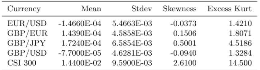
Table 1 summarizes descriptive statistics for daily returns for the full sample. Panel A reports the mean, standard deviation, skewness and excess kurtosis while Panel B tabulates the autocorre-lation coefficients and the Ljung and Box (1978) statistic for autocorreautocorre-lation for the first five lags. The p-values for the Ljung-Box statistic are reported in parentheses. In the Ljung-Box test, the null hypothesis of no autocorrelation is strongly rejected. In Figure 2, we plot the autocorrelation of daily realized volatility for up to 30 lags for the assets.
4
Empirical analyses
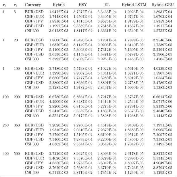
In Table 2, we summarize the RMSFE of realized volatility for the Hybrid, HSY, and EL models over six forecast horizons for all assets. We observe that in this comparison of point estimates, the Hybrid model shows very strong performance and dominates the other models in producing the smallest RMSFE, usually by a big margin, except for two occassions whereby the HSY is the best-performing model for GBP/EUR over the shortest forecasting horizon and for the CSI index for the horizon between 1 and 100 days. Our results are consistent with evidence in the literature that the artificial neural network is able to produce significantly more accurate forecast when applied to deseasonalized data (Nelson et al., 1999; Zhang and Qi, 2005).
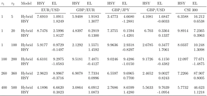
We conduct the Diebold and Mariano (1995) pairwise comparison between the forecasting dif-ference of alternative volatility models and report the heteroscedasticity- and serial correlation-adjusted t-statistics in Table 3. A positive t-statistic indicates that the model in the row is pre-ferred to the model in the column while a negativet-statistic suggests that the model in the column is preferred. We note that between the Hybrid and the HSY models, the Hybrid model is always preferred with significant t-statistic. It is often preferred when compared with the EL model, es-pecially over longer horizons. The forecasting performances of the HSY and the EL models are similar on statistical terms.
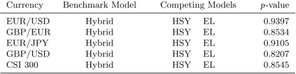
We implement the superior predicative ability (SPA) test of Hansen (2005) and tabulate the stationary bootstrappedp-values, obtained via 1000 replications, in Table 4.5 The null hypothesis that the benchmark model is not inferior to any of the competing models is resoundingly accepted with a highp-value when the Hybrid is the benchmark model.6
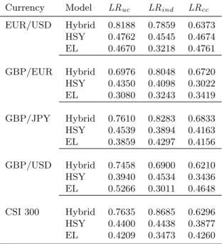
In Table 5, we undertake the likelihood ratio tests formulated in Christoffersen (1998) and report thep-values for the null hypotheses that at the 5% level the volatility forecasts exhibit the correct unconditional coverage LRuc, are independent LRind, and exhibit the correct conditional
coverage LRcc, respectively. Not surprisingly, the Hybrid model passes the test with flying colors and exhibits the highest p-values between 0.62 and 0.87. This once again attests to the accuracy and adequacy of the volatility forecasts of our proposed model. For the HSY and EL models, the
5
We aggregate volatility forecasts over all six horizons for each currency in order to provide a comprehensive and clear picture.
6We also conduct the Mincer and Zarnowitz (1969) regression, which shows the ability of the forecasted volatility in explaining the true volatility proxy. We find that the R2 decreases massively with increasing forecast horizons for all models as expected. However, our proposed Hybrid model still shows 30% to 70% explanatory power for the longest forecast horizon and comes out stronger than the competing models. These results are available upon request from the authors.
null is accepted with much lower p-values typically between 0.30 and 0.53.
To summarize, in our baseline analysis we conduct a number of statistical tests to evaluate the out-of-sample performance of our neural network enhanced model and alternative two-component models. Our proposed model substantially outperforms the others in these econometric tests.
4.1 Forecasting error analysis
What drives the superior forecasting performance of our proposed model? To obtain a better understanding of the differences in the empirical performance between the models, we break down and analyze the forecasting errors for each component across the three models.
In Figure 3, we plot in Panels (a) and (b) the average absolute percentage error (APE) of the short- and long-term components, respectively, for EUR/USD for the three models. In Panel (a), the Hybrid model exhibits the smallest forecasting error for the short-term component, followed by the EL model, and the HSY on average offers the largest forecasting errors. Nevertheless, the errors for the short-term component are not too different from each other across the models and typically lie between 10% and 35%. However, Panel (b) shows a very different pattern. Over the two shortest horizons of up to 20 days, all models produce quite accurate forecasts and the APE is less than 1%. But as we move to longer horizons, we see massive difference between the APE for the long-term component: for the Hybrid model the APE is less than 2%, whereas for the EL and the HSY, it goes up to 23% and 28%, respectively. So it is the precision of the long-term component that drives the distinct performance of the models and this underlines the prowess of the neural network in capturing the trend component in time series of data.7
In Table 6, we report the average APE in percent for all test assets. The same pattern emerges that our neural network enhanced model shows extraordinary ability in capturing the trend and producing average APE of 1.47% at most even for the 16-month horizon. For the other two models, the average APE is somewhere between 15% and 32% for the long-term component over the longest forecasting horizon.
4.2 Robustness check
Alternative volatility proxy
We perform a number of robustness tests to show that our baseline results are not due to
7
It is worth noting that the artificial neural network does not work well on modeling and forecasting the overall volatility dynamics. See Yao et al. (2017) for example.
specific modeling choices. First, instead of using realized volatility we adopt the intraday range-based measure for volatility modeling and as the proxy for true volatility. The range-range-based measure is proven robust to microstructure noise and receives renewed interest in the literature in recent years (Alizadeh et al., 2002; Engle and Gallo, 2006). It is specified as follows:
σ2t = 1
4 ln 2(P
H
t −PtL)2, (12)
wherePtH andPtL are the highest and lowest prices on dayt, respectively.
Table A1 in the online appendix reports the summary statistics for the daily range-based volatil-ity for the full sample. In Table 7, we tabulate the p-values for the SPA test when volatilities are measured as the squared range between the highest and lowest prices in a day. We observe the same pattern that the Hybrid model is not inferior to the competing HSY and EL models with similarly highp-values as those obtained in our baseline results in Table 4.
Alternative loss function for volatility prediction accuracy
Our second robustness check is to adopt the loss function, QLIKE, between the true and fore-casted volatility. It is defined as follows:
QLIKE= log ˆσ2+σ
2
ˆ
σ2, (13)
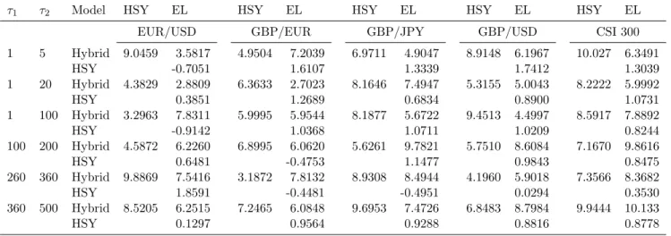
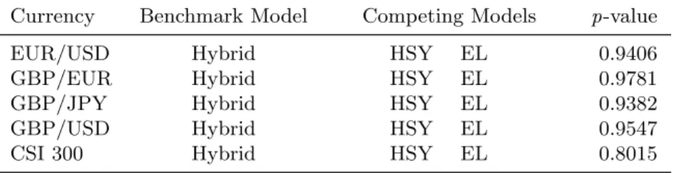
where ˆσ2 and σ2 are variance forecasts and the true variance proxy, respectively. This particular loss function, robust when the proxy is unbiased but imperfect, is recommended in Patton (2011) and Bollerslev et al. (2016b). In Table 8, we report the heteroscedasticity- and serial correlation-adjusted t-statistic for the Diebold and Mariano (1995) pairwise comparison withQLIKE as the loss function. We find that at the Hybrid model is always preferred to the HSY and EL models. We further conduct the SPA test of Hansen (2005) on range-based volatility with the QLIKE as the loss function and summarize the results in Table 9. We obtain qualitatively similar results to the baseline findings. The null hypothesis is always accepted with very high p-value.
Alternative model for the long-term component
Our paper proposes a framework in which adopting advanced neural network models for describ-ing the long-term component helps generate more precise volatility forecasts. Hence, the volatility forecasting accuracy is not expected to be greatly affected by the specific neural network model we choose. In the third robustness test, we implement two popular neural network models, i.e.,
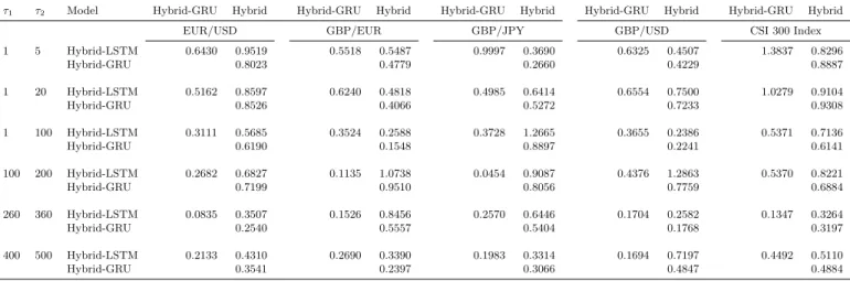
the long short-term memory model (LSTM) (Gers et al., 2000; Hochreiter and Schmidhuber, 1997) and the gated recurrent unit (GRU) model (Cho et al., 2014; Chung et al., 2014) for the long-term component, and call them the Hybrid-LSTM and Hybrid-GRU, respectively. The forecasting errors for these models are summarized in the last two columns in Table 2, and the Diebold and Mari-ano (1995) pairwise comparison results are reported in Table 10. Consistent with our conjecture, performance of these three hybrid models are statistically comparable as the t-statistic is always insignificant.
To summarize, the empirical results in the robustness tests further corroborate the baseline findings that the neural network enhanced volatility model outperforms the two-component models of Harris et al. (2011) and Engle and Lee (1999) in producing more accurate volatility predictions over different horizons for all test assets.8 This attests to the validity of proposed framework that neural network enhanced component volatility models generate more precise volatility predictions.
4.3 Economic value of volatility forecasts
A strong statistical performance does not necessarily indicate superior economic significance in the out-of-sample exercise. Therefore we analyze the economic value of volatility forecasts assuming a mean-variance utility investor who allocates her wealth between a risk-free asset and one of the four exchange rates or the stock index. We follow Wang et al. (2016) to construct the utility function as follows: Ut(rt) =Et(wtrt+rt,f)− 1 2γσ 2 t (wtrt+rt,f), (14)
wherewt is the weight of the risky asset in the portfolio,rt is the return to the risky asset in excess
of the risk-free rate,rt,f, andγ denotes the level of risk aversion. We maximize the utility function Ut(rt) with respect to the weightwt and obtain the ex ante optimal weight on day t+ 1:
ˆ wt= 1 γ ˆ rt+1 ˆ σ2 t+1 , (15)
where ˆrt+1 and ˆσt2+1 are the mean and volatility forecasts, respectively, of the excess returns. In
our study, risk-free rates come from the three-month US Treasury bill or the three-month Chinese national bond yield.
8
We have conducted yet another robustness check by adopting the low-pass Hodrick and Prescott (1997) filter and see whether the performance of the Hybrid model is due to our choice of the particular decomposition method, i.e. the wavelet method. We obtain qualitatively similar results that the model with the Hodrick and Prescott (1997) filtering, with the long-/short-term component still modelled via the artificial neural network and the ARMA process,
Following Rapach et al. (2010) and Wang et al. (2016), we use the historical average as the mean forecasts for returns, ˆrt+1 =Ptj=1rj. Hence, for each level of risk aversion γ, the optimal
weight ˆwt = γ1 rˆ t+1 ˆ σ2 t+1
of the portfolio is only determined by the volatility forecasts as different strategies share the same mean forecasts of returns. We use the Sharpe ratio (SR):
SR = µp¯ ¯
σp (16)
and the certainty equivalent return (CER):
CER = ˆµp−γ
2σˆ
2
p (17)
to evaluate the performance of a portfolio, where ¯µp and ¯σp are the mean and standard deviation
of portfolio excess returns, respectively; ˆµp and ˆσp2 are the mean and variance of portfolio returns in the out-of-sample period, respectively. For robustness, we adopt γ=3, 6, and 9 to represent different level of risk aversion.
In Table 11, we report the annualized average return, the Sharpe ratio, and the CER of the portfolios constructed using realized volatility from different models. When the investor is assumed to have a relatively low level of risk aversion atγ=3, portfolios are able to achieve an annual return of 6.63% when volatility forecasts are generated by the Hybrid model for EUR/USD, and the Sharpe ratio is 0.37, while the certainty equivalent return is slightly higher than 3%. These are evidently higher than when the forecasts are generated by the competing models. As the investor becomes more risk averse with largerγ value, she assigns a greater weight to the risk-free asset. This results in lower portfolio return, Sharpe ratio and the CER. Nevertheless, the same pattern exists that the portfolios formed using the Hybrid volatility forecasts offer higher return and risk-adjusted return, substantiating the economic value of the volatility forecasts from our proposed model.
Meanwhile, given the inextricable link between the macroeconomy and financial market volatil-ity, especially the long-term component of the volatility dynamics (see Bloom, 2009; Chiu et al., 2018; Conrad et al., 2014; Engle et al., 2013, for example), we perform a vector autoregression to explore how the macroeconomic conditions impact on the persistent component of exchange rates. In particular, we examine the impulse response of the long-term component of EURUSD and GBPUSD to changes in two important US macroeconomic variables: the GDP growth and the Federal fund rate. We find that for both exchange rates, the long-term volatility trends down given a disturbance to the GDP growth over the next five months but picks up in the medium run,
whereas a shock to the Federate fund rate increases the long-term component of volatility over the next five to ten months.9
5
Conclusion
The evidence that conditional volatility dynamics comprises both a long-term trend component and a strongly oscillating short-run component has crucial implication for volatility forecasting over both short and long horizons. In this paper, we build upon and extend the two-component volatility literature and develop a novel neural network enhanced volatility component model. We first decompose the daily realized volatility into long- and short-run components using the wavelet transform while implementing the ADF test to choose appropriate parameters and ensuring the stationarity assumption for the short-run component is satisfied. We then separately model the long- and short-run components with the artificial neural network and an ARMA model, respec-tively. The model is empirically evaluated using data on four exchange rates and a stock index over a number of forecast horizons. We compare the RMSFE and perform statistical evaluations such as the Diebold and Mariano (1995) test, the SPA test of Hansen (2005), and the interval fore-cast evaluation of Christoffersen (1998). In the out-of-sample comparison of volatility predictions generated by our proposed model and popular alternative models, we provide strong and robust evidence that our neural network enhanced model significantly outperforms the competing models. In economic terms, the volatility forecasts from the Hybrid model offers improved economic value to a mean-variance utility investor.
Appendix
Specifications for competing volatility models
Two-component model of Harris et al. (2011)In Harris et al. (2011), the volatility follows a two-factor process specified as follows:
σt=qt+α(σt−1−qt−1) +t, (A1)
9
whereqtis the long-run trend component of the volatility, the short-term component is defined as σt−qt, andtis a random error term with zero mean and constant variance. The model assumes the long-run trend follows a random walk over the forecast horizon so that E[qt+i|t] =qtfor all i >0.
The two components are obtained via two nonparametric filters: the low-pass filter of Hodrick and Prescott (1997) and the band-pass filter of Christiano and Fitzgerald (2003).
The Component GARCH model
The two-component volatility model of Engle and Lee (1999) for returns over time period t,rt, is given as follows: rt = p htt (A2) ht = τt+gt (A3) τt = ω+ρτt−1+φ(r2t−1−ht−1) (A4) gt = α(r2t−1−τt−1) +βgt−1, (A5)
wheretis ani.i.d series of standardized random variables. The variancehtis decomposed intoτt,
References
Adrian, T., Rosenberg, J., 2008. Stock returns and volatility: Pricing the short-run and long-run components of market risk. Journal of Finance 63, 2997–3030.
Alizadeh, S., Brandt, M., Diebold, F., 2002. Range-based estimation of stochastic volatility models. Journal of Finance 57, 1047–1091.
Andersen, T. G., Bollerslev, T., 1998. Answering the skeptics: Yes, standard volatility models do provide accurate forecasts. International Economic Review 39, 885–905.
Barunik, J., Krehlik, T., Vacha, L., 2016. Modeling and forecasting exchange rate volatility in time-frequency domain. European Journal of Operational Research 251, 329–340.
Bloom, N., 2009. The impact of uncertainty shocks. Econometrica 77, 623–685.
Bollerslev, T., 1986. Generalized autoregressive conditional heteroskedasticity. Journal of Econo-metrics 31, 307–327.
Bollerslev, T., Li, S. Z., Todorov, V., 2016a. Roughing up beta: Continuous versus discontinuous betas and the cross section of expected stock returns. Journal of Financial Economics 120, 464– 490.
Bollerslev, T., Patton, A. J., Quaedvlieg, R., 2016b. Exploiting the errors: A simple approach for improved volatility forecasting. Journal of Econometrics 192, 1–18.
Brandt, M. W., Jones, C. S., 2006. Volatility forecasting with range-based EGARCH models. Journal of Business & Economic Statistics 24, 470–486.
Breaban, A., Noussair, C. N., 2018. Emotional state and market behavior. Review of Finance 22, 279–309.
Chiu, C.-W. J., Harris, R. D., Stoja, E., Chin, M., 2018. Financial market volatility, macroeconomic fundamentals and investor sentiment. Journal of Banking & Finance 92, 130–145.
Cho, K., Van Merri¨enboer, B., Bahdanau, D., Bengio, Y., 2014. On the properties of neural machine translation: Encoder-decoder approaches, arXiv preprint arXiv: 1409.1259.
Christoffersen, P. F., 1998. Evaluating interval forecasts. International Economic Review 39, 841– 862.
Christoffersen, P. F., Pelletier, D., 2004. Backtesting Value-at-Risk: A duration-based approach. Journal of Financial Econometrics 2, 84–108.
Chung, J., Gulcehre, C., Cho, K., Bengio, Y., 2014. Empirical evaluation of gated recurrent neural networks on sequence modeling, arXiv preprint arXiv: 1412.3555.
Colacito, R., Engle, R. F., Ghysels, E., 2011. A component model for dynamic correlations. Journal of Econometrics 164, 45–59.
Conrad, C., Loch, K., Rittler, D., 2014. On the macroeconomic determinants of long-term volatili-ties and correlations in US stock and crude oil markets. Journal of Empirical Finance 29, 26–40. Corsi, F., 2009. A simple approximate long-memory model of realized volatility. Journal of Financial
Econometrics 7, 174–196.
Daubechies, I., 1992. Ten Lectures on Wavelets. Philadelphia: Socienty for Industrial and Applied Mathematics.
Diebold, F., Mariano, R. S., 1995. Comparing predictive accuracy. Journal of Business & Economic Statistics 13, 253–263.
Engle, R., 1982. Autoregressive conditional heteroscedasticity with estimates of the variance of United Kingdom inflation. Econometrica 50, 987–1007.
Engle, R. F., Gallo, G. M., 2006. A multiple indicators model for volatility using intra-daily data. Journal of Econometrics 131, 3–27.
Engle, R. F., Ghysels, E., Sohn, B., 2013. Stock market volatility and macroeconomic fundamentals. Review of Economics and Statistics 95, 776–797.
Engle, R. F., Lee, G., 1999. A long-run and short-run component model of stock return volatility. In: Engle, R., White, H. (Eds.), Cointegration, Causality, and Forecasting: A Festschrift in Honour of Clive WJ Granger. Oxford University Press, pp. 475–497.
Engle, R. F., Rangel, J. G., 2008. The spline-GARCH model for low-frequency volatility and its global macroeconomic causes. Review of Financial Studies 21, 1187–1222.
Engle, R. F., Sokalska, M. E., 2012. Forecasting intraday volatility in the US equity market. Mul-tiplicative component GARCH. Journal of Financial Econometrics 10, 54–83.
Esteban-Bravo, M., Vidal-Sanz, J. M., 2007. Computing continuous-time growth models with boundary conditions via wavelets. Journal of Economic Dynamics & Control 31, 3614–3643. Fuller, W. A., 1976. Introduction to Statistical Time Series. John Wiley & Sons.
Garcia, R., Gencay, R., 2000. Pricing and hedging derivative securities with neural networks and a homogeneity hint. Journal of Econometrics 94, 93–115.
Gers, F., Schmidhuber, J., Cummins, F., 2000. Learning to forget: Continual prediction with LSTM. Neural computation 12, 24–51.
Granger, C. W. J., 1980. Long memory relationships and the aggregation of dynamic models. Journal of Econometrics 14, 227–238.
Hagan, M., Menhaj, M., 1994. Training feedforward networks with the Marquardt algorithm. IEEE Transactions on Neural Networks 5, 989–993.
Hansen, P. R., 2005. A test of superior predictive ability. Journal of Business & Economic Statistics 23, 365–380.
Harris, R., Stoja, E., Yilmaz, F., 2011. A cyclical model of exchange rate volatility. Journal of Banking & Finance 35, 3055–3064.
Haven, E., Liu, X., Ma, C., Shen, L., 2009. Revealing the implied risk-neutral MGF from options: The wavelet method. Journal of Economic Dynamics & Control 33, 692–709.
Haven, E., Liu, X., Shen, L., 2012. De-noising option prices with the wavelet method. European Journal of Operational Research 222, 104–112.
Hochreiter, S., Schmidhuber, J., 1997. Long short-term memory. Neural computation 9, 1735–1780. Hodrick, R., Prescott, E., 1997. Post-war US business cycles: An empirical investigation. Journal
of Money, Credit and Banking 29, 1–16.
Hutchinson, J. M., Lo, A., Poggio, T., 1994. A nonparametric approach to pricing and hedging derivative securities via learning networks. Journal of Finance 49, 851–889.
Kristjanpoller, W., Fadic, A., Minutolo, M. C., 2014. Volatility forecast using hybrid neural network models. Expert Systems with Applications 41, 2437–2442.
Kristjanpoller, W., Minutolo, M., 2016. Forecasting volatility of oil price using an artificial neural network-GARCH model. Expert Systems with Applications 65, 233–241.
Kristjanpoller, W., Minutolo, M. C., 2015. Gold price volatility: A forecasting approach using the artificial neural network-GARCH model. Expert Systems with Applications 42, 7245–7251. Liu, F., Pantelous, A. A., Von Mettenheim, H.-J., 2018. Forecasting and trading high frequency
volatility on large indices. Quantitative Finance 18, 737–748.
Ljung, G. M., Box, G. E. P., 1978. On a measure of a lack of fit in time series models. Biometrika 65, 297–303.
Mandic, D., Chambers, J., 2001. Recurrent Neural Networks for Prediction. John Wiley & Sons. McQuarrie, A. D., Tsai, C.-L., 1998. Regression and Time Series Model Selection. Singapore: World
Scientific.
Mincer, J., Zarnowitz, V., 1969. The evaluation of economic forecasts. In: Zarnowitz, J. (Ed.), Economic Forecasts and Expectations. National Bureau of Economic Research, New York. Mustafaraj, G., Lowery, G., Chen, J., 2011. Prediction of room temperature and relative humidity
by autoregressive linear and nonlinear neural network models for an open office. Energy and Buildings 43, 1452–1460.
Nelson, D., 1991. Conditional heteroskedasticity in asset returns: A new approach. Econometrica 59, 347–370.
Nelson, M., Hill, T., Remus, W., O’Conner, M., 1999. Time series forecasting using NNs: Should the data be deseasonalized first? Journal of Forecasting 18, 359–367.
Norgaard, M., Rawn, O., Poulsen, N., Hansen, L., 2000. Neural Network for Modeling and Control of Dynamic Systems. Springer-Verlag.
Nrgaard, M., Ravn, O. E., Poulsen, N. K., Hansen, L. K., 2000. Neural Networks for Modelling and Control of Dynamic Systems: A Practitioner’s Handbook, 1st Edition. Springer-Verlag, Berlin, Heidelberg.
Patil, S., Tantau, H., Salokhe, V., 2008. Modelling of tropical greenhouse temperature by autore-gressive and neural network models. Biosystems Engineering 99, 423–431.
Patton, A., 2011. Volatility forecast comparison using imperfect volatility proxies. Journal of Econo-metrics 160, 246–256.
Rapach, D. E., Strauss, J. K., Zhou, G., 2010. Out-of-sample equity premium prediction: Combi-nation forecasts and links to the real economy. Review of Financial Studies 23, 821–862.
Schwarz, G., 1978. Estimating the dimension of a model. Annals of Statistics 6, 461–464.
Shephard, N., 1996. Statistical aspects of ARCH and stochastic volatility. In: Cox, D. R., Hinkley, D. V., Barndorff-Nielsen, O. E. (Eds.), Time Series Models: In econometrics, finance and other applications. Chapman & Hall/CRC Monographs on Statistics and Applied Probability, London, pp. 1–68.
Siegelmann, H., Horne, B., Giles, C., 1997. Computational capabilities of recurrent NARX neural networks. IEEE Transactions on Systems, Man, and Cybernetics, Part B(Cybernetics) 27, 208– 215.
Taylor, S. J., 1994. Modelling stochastic volatilitiy: A review and comparative study. Mathematical Finance 4, 183–204.
Wang, F., Ghysels, E., 2015. Econometric analysis of volatility component models. Econometric Theory 31, 362–393.
Wang, Y., Ma, F., Wei, Y., Wu, C., 2016. Forecasting realized volatility in a changing world: A dynamic model averaging approach. Journal of Banking & Finance 64, 136–149.
Yao, Y., Zhai, J., Cao, Y., Ding, X., Liu, J., Luo, Y., 2017. Data analytics enhanced component volatility model. Expert Systems with Applications 84, 232–241.
Zhang, P., Qi, M., 2005. Neural network forecasting for seasonal and trend time series. European Journal of Operational Research 160, 501–514.
Table 1. Descriptive statistics for daily returns
This table summarizes the mean, standard deviation, skewness, excess kurtosis, and autocorrelations for daily returns to exchange rates and the stock index. Thep-values for the Ljung-Box test are reported in parentheses. The sample period is from 27 Sept 2009 to 12 Aug 2015 for the exchange rates and from 1 August 2005 to 29 September 2017 for the CSI 300 index.
Panel A. Summary statistics
Currency Mean Stdev Skewness Excess Kurt
EUR/USD -1.4660E-04 5.4663E-03 -0.0373 1.4210
GBP/EUR 1.4390E-04 4.5858E-03 0.1506 1.8071
GBP/JPY 1.7240E-04 6.5854E-03 0.5001 4.5186
GBP/USD -7.7000E-05 4.6281E-03 -0.0940 1.3284
CSI 300 1.4400E-02 9.5900E-03 2.6100 14.500
Panel B. Autocorrelation
Currency Lag 1 Lag 2 Lag 3 Lag 4 Lag 5 Ljung-Box test
EUR/USD 3.62E-02 -1.13E-02 -2.67E-02 -9.63E-03 1.24E-03 2.4200 (0.1200)
GBP/EUR 2.65E-02 -4.68E-02 -6.74E-02 7.64E-04 -1.62E-02 1.2900 (0.2560)
GBP/JPY 2.80E-04 -3.00E-02 -6.40E-02 1.28E-04 5.03E-02 0.0014 (0.9900)
GBP/USD -2.57E-02 -3.77E-02 7.55E-03 2.20E-03 -1.38E-02 1.2100 (0.2710)
Table 2. The forecasting accuracy of alternative volatility models
This table reports the root mean squared forecasting error (RMSFE) for the neural network enhanced model (Hybrid), the cyclical model of Harris et al. (2011) (HSY), and the component GARCH of Engle and Lee (1999)(EL). The RMSFE is also reported when the long-term component is modeled by the LSTM model (Hybrid-LSTM) or the GRU model (Hybrid-GRU). The out-of-sample period is from 8 December 2012 to 15 August 2015 for exchange rates, and from 1 August 2008 to 29 September 2017 for the CSI 300 index. The forecasting horizon is from dayt+τ1to dayt+τ2.
τ1 τ2 Currency Hybrid HSY EL Hybrid-LSTM Hybrid-GRU
1 5 EUR/USD 1.9472E-04 3.7272E-04 5.3433E-04 1.9023E-04 1.8931E-04
GBP/EUR 1.7448E-04 1.4507E-04 9.3405E-04 1.6747E-04 1.6762E-04
GBP/JPY 1.8910E-04 6.1415E-04 6.6625E-04 1.8129E-04 1.8359E-04
GBP/USD 1.1997E-04 9.5389E-04 4.7618E-04 1.1637E-04 1.1917E-04
CSI 300 3.0428E-03 1.8117E-02 1.3661E-02 1.6540E-03 1.5752E-03
1 20 EUR/USD 1.8600E-06 4.8420E-04 6.1201E-04 1.7829E-06 3.9546E-06
GBP/EUR 1.6370E-05 8.1149E-04 2.0203E-04 1.6140E-05 1.7539E-05
GBP/JPY 5.4100E-05 5.3093E-04 7.7312E-04 5.1605E-05 5.2294E-05
GBP/USD 3.6530E-05 4.1159E-04 4.6871E-04 3.5787E-05 3.5966E-05
CSI 300 2.3797E-03 6.7069E-03 8.9285E-03 1.4485E-03 1.4705E-03
1 100 EUR/USD 3.7480E-05 5.5738E-04 8.1022E-04 3.5610E-05 4.0239E-05
GBP/EUR 1.3290E-05 7.2007E-04 6.4341E-04 1.3271E-05 1.5907E-05
GBP/JPY 8.6800E-06 7.7477E-04 4.3280E-04 8.5912E-06 1.0554E-05
GBP/USD 2.3800E-05 1.8636E-04 6.8801E-04 2.2758E-05 2.4789E-05
CSI 300 5.1285E-03 1.9782E-03 2.8437E-03 1.6060E-03 1.5383E-03
100 200 EUR/USD 6.6780E-05 6.8664E-04 5.7217E-04 6.5737E-05 6.6614E-05
GBP/EUR 4.2900E-06 8.3487E-04 6.1414E-04 4.2544E-06 5.0717E-06
GBP/JPY 2.8200E-06 6.8156E-04 5.2273E-04 2.7291E-06 5.2139E-06
GBP/USD 2.5410E-05 5.8532E-04 1.1835E-04 2.5375E-05 2.4840E-05
CSI 300 6.5524E-03 5.0172E-02 4.5828E-02 1.1268E-03 1.1443E-03
260 360 EUR/USD 7.2020E-05 7.2760E-04 4.4519E-04 6.9409E-05 7.1971E-05
GBP/EUR 1.9310E-05 2.0510E-04 7.2379E-04 1.8586E-05 2.0965E-05
GBP/JPY 7.2790E-05 1.5105E-04 8.6109E-04 6.9512E-05 7.2097E-05
GBP/USD 7.5100E-05 7.2893E-04 9.2200E-04 7.4866E-05 7.3583E-05
CSI 300 4.6362E-03 2.3344E-02 3.0649E-02 1.7042E-03 1.7497E-03
400 500 EUR/USD 2.7220E-05 8.9625E-04 4.8093E-04 2.6178E-05 2.8225E-05
GBP/EUR 5.4620E-05 7.3370E-04 2.6279E-04 5.2996E-05 5.5345E-05
GBP/JPY 4.8850E-05 1.9753E-04 3.6042E-04 4.8097E-05 4.9049E-05
GBP/USD 3.7620E-05 2.5680E-04 3.3710E-04 3.7423E-05 3.8794E-05
Table 3. The Diebold and Mariano (1995) t-statistics
This table reports the heteroscedasticity- and serial correlation-adjusted t-statistics for the Diebold and Mariano (1995) pairwise comparison for out-of-sample forecasts between volatility models. A positive t-statistic indicates that the model in the row is preferred to the one in the column and a negativet-statistic indicates that the model in the column is preferred. The out-of-sample period is from 8 December 2012 to 15 August 2015 for the exchange
rates and from 1 August 2008 to 29 September 2017 for the CSI 300 index. The forecast horizon is from dayt+τ1
to dayt+τ2.
τ1 τ2 Model HSY EL HSY EL HSY EL HSY EL HSY EL
EUR/USD GBP/EUR GBP/JPY GBP/USD CSI 300 1 5 Hybrid 7.6910 1.0911 5.9408 1.9183 3.4773 4.6680 4.1081 1.6847 6.3588 16.212 HSY 1.8249 1.3077 -1.2881 -0.6033 0.6538 1 20 Hybrid 8.7476 2.5996 4.8397 0.2919 7.3755 0.1594 6.703 0.3364 9.8914 7.2365 HSY 1.8127 0.1300 -1.4201 0.1337 0.3963 1 100 Hybrid 5.9177 0.9729 2.1292 1.5571 9.9636 2.9318 2.6785 0.3477 8.0337 10.248 HSY -0.1497 1.4592 -0.8297 1.7061 1.3098 100 200 Hybrid 6.6101 9.2975 9.5181 7.4871 9.0246 9.4286 9.1726 6.1150 12.097 77.671 HSY -1.0583 -0.4127 -1.0150 -0.4382 -1.4875 260 360 Hybrid 2.9623 8.9967 6.9078 7.7334 6.5597 9.6965 2.4652 9.0027 7.2266 87.907 HSY -0.3716 0.0996 0.7700 0.8243 0.8005 400 500 Hybrid 4.1896 6.6620 3.0864 6.0912 2.7686 8.6599 5.5633 9.7639 5.7732 46.623 HSY 0.3823 1.0873 1.4280 -1.0954 1.1218
Table 4. The superior predicative ability (SPA) test of Hansen (2005)
This table reports the Hansen (2005) SPA test results for out-of-sample volatility forecasts based on the RMSFE.
The benchmark model is the Hybrid model. The out-of-sample period is from 8 December 2012 to 15 August
2015 for the exchange rates and from 1 August 2008 to 29 September 2017 for the CSI 300 index. The stationary bootstrappedp-values are obtained via 1000 replications.
Currency Benchmark Model Competing Models p-value
EUR/USD Hybrid HSY EL 0.9397
GBP/EUR Hybrid HSY EL 0.8534
EUR/JPY Hybrid HSY EL 0.9105
GBP/USD Hybrid HSY EL 0.8207
Table 5. Interval evaluation of volatility forecasts
This table reports thep-values of the Christoffersen (1998) interval forecast evaluation with the null hypothesis of correct coverageH0:f= 5%. These include the likelihood ratio of unconditional coverageLRuc, the likelihood ratio
of independenceLRind, and the likelihood ratio of conditional coverageLRcc. The out-of-sample period is from 8
December 2012 to 15 August 2015 for the exchange rates and from 1 August 2008 to 29 September 2017 for the CSI 300 index.
Currency Model LRuc LRind LRcc
EUR/USD Hybrid 0.8188 0.7859 0.6373 HSY 0.4762 0.4545 0.4674 EL 0.4670 0.3218 0.4761 GBP/EUR Hybrid 0.6976 0.8048 0.6720 HSY 0.4350 0.4098 0.3022 EL 0.3080 0.3243 0.3419 GBP/JPY Hybrid 0.7610 0.8283 0.6833 HSY 0.4539 0.3894 0.4163 EL 0.3859 0.4297 0.4156 GBP/USD Hybrid 0.7458 0.6900 0.6210 HSY 0.3940 0.4534 0.3436 EL 0.5266 0.3011 0.4648 CSI 300 Hybrid 0.7635 0.8685 0.6296 HSY 0.4400 0.4438 0.3877 EL 0.4209 0.3473 0.4260
Table 6. Volatility forecasting error analysis
This table reports the average absolute percentage error (APE) in percent of the long- and short-term components of volatility forecasts by the neural network enhanced model (Hybrid), the cyclical model of Harris et al. (2011) model (HSY), and the component GARCH of Engle and Lee (1999)(EL) over different forecasting horizons. The out-of-sample period is from 8 December 2012 to 15 August 2015 for the exchange rates and from 1 August 2008 to 29 September 2017 for the CSI 300 index. The forecast horizon is from dayt+τ1 to dayt+τ2.
Currency τ1 τ2 HSY LT HSY ST EL LT EL ST Hybrid LT Hybrid ST
EUR/USD 1 5 0.2628 34.407 0.8229 25.877 0.0731 12.931 1 20 0.9122 34.459 0.8095 24.537 0.0483 16.326 1 100 4.6594 30.516 3.2042 26.723 0.0784 12.622 100 200 23.829 23.088 13.454 24.925 0.0117 8.7000 260 360 20.716 29.686 19.143 26.603 0.0260 15.738 400 500 28.346 23.918 21.681 23.294 0.8634 9.7544 GBP/EUR 1 5 0.6066 26.851 0.8923 29.145 0.0961 12.486 1 20 0.4939 31.201 0.4922 26.311 0.0806 13.170 1 100 3.7014 31.629 4.4049 22.591 0.1086 11.088 100 200 23.326 23.528 16.110 22.236 0.0590 10.388 260 360 11.457 24.254 16.843 22.189 0.1083 11.148 400 500 29.375 24.502 25.182 29.769 1.3931 8.5424 GBP/JPY 1 5 0.4931 22.640 0.6058 27.431 0.0310 14.133 1 20 0.2197 25.788 0.8384 22.447 0.0582 15.069 1 100 5.4097 26.420 3.9443 26.874 0.1092 15.236 100 200 17.045 29.865 21.506 29.998 0.0646 12.184 260 360 21.970 31.153 13.065 23.162 0.0127 12.711 400 500 17.467 29.353 16.698 28.497 0.8957 13.101 GBP/USD 1 5 0.4507 22.102 0.8923 26.239 0.1089 15.924 1 20 1.0454 28.054 0.4939 27.121 0.0140 14.818 1 100 2.9916 26.621 4.0927 24.109 0.0300 17.533 100 200 13.030 29.968 18.911 24.768 0.0176 11.413 260 360 16.254 33.174 19.835 27.936 0.0296 15.761 400 500 32.017 27.588 17.707 24.676 1.4686 8.9945 CSI 300 1 5 0.3607 20.813 0.5679 19.691 0.0567 10.876 1 20 0.5293 23.326 0.4962 18.570 0.0368 10.457 1 100 3.2654 21.381 2.7823 18.837 0.0609 10.317 100 200 14.636 20.702 12.642 18.576 0.0300 8.2616 260 360 13.291 22.744 13.666 19.076 0.0351 9.9418 400 500 21.130 20.491 15.499 19.035 0.9195 7.6124
Table 7. Robustness test: The superior predicative ability (SPA) test of Hansen (2005) on range-based volatility
This table reports the Hansen (2005) SPA test results based on the RMSFE and intraday range-based volatility. The benchmark model is the Hybrid model. The out-of-sample period is from 8 December 2012 to 15 August 2015 for the exchange rates and from 1 August 2008 to 29 September 2017 for the CSI 300 index. The stationary bootstrapped p-values are obtained via 1000 replications.
Currency Benchmark Model Competing Models p-value
EUR/USD Hybrid HSY EL 0.9210
GBP/EUR Hybrid HSY EL 0.8947
GBP/JPY Hybrid HSY EL 0.9209
GBP/USD Hybrid HSY EL 0.9145
Table 8. Robustness test: The Diebold and Mariano (1995)t-statistics withQLIKE as loss function
This table reports the the heteroscedasticity- and serial correlation-adjustedt-statistics for the Diebold and Mariano
(1995) pairwise comparison for out-of-sample forecasts when the loss function is QLIKE. A positive t-statistic
indicates that the model in the row is preferred to that in the column and a negativet-statistic indicates that the model in the column is preferred. The out-of-sample period is from 8 December 2012 to 15 August 2015 for the exchange rates and from 1 August 2008 to 29 September 2017 for the CSI 300 index. The forecast horizon is from dayt+τ1 to dayt+τ2.
τ1 τ2 Model HSY EL HSY EL HSY EL HSY EL HSY EL
EUR/USD GBP/EUR GBP/JPY GBP/USD CSI 300 1 5 Hybrid 9.0459 3.5817 4.9504 7.2039 6.9711 4.9047 8.9148 6.1967 10.027 6.3491 HSY -0.7051 1.6107 1.3339 1.7412 1.3039 1 20 Hybrid 4.3829 2.8809 6.3633 2.7023 8.1646 7.4947 5.3155 5.0043 8.2222 5.9992 HSY 0.3851 1.2689 0.6834 0.8900 1.0731 1 100 Hybrid 3.2963 7.8311 5.9995 5.9544 8.1877 5.6722 9.4513 4.4997 8.5917 7.8892 HSY -0.9142 1.0368 1.0711 1.0209 0.8244 100 200 Hybrid 4.5872 6.2260 6.8995 6.0620 5.6261 9.7821 5.7510 8.6084 7.1670 9.8616 HSY 0.6481 -0.4753 1.1477 0.9843 0.8475 260 360 Hybrid 9.8869 7.5416 3.1872 7.8132 8.9308 8.4944 4.1960 5.9018 7.3566 8.3682 HSY 1.8591 -0.4481 -0.4951 0.0294 0.3530 360 500 Hybrid 8.5205 6.2515 7.2465 6.0848 9.6953 7.4726 6.8483 8.7984 9.9444 10.133 HSY 0.1297 0.9564 0.9288 0.8816 0.8778
Table 9. Robustness: The superior predicative ability (SPA) test of Hansen (2005) on range-based volatility withQLIKE as loss function
This table reports the Hansen (2005) SPA test results for out-of-sample range-based volatility forecasts when the
loss function isQLIKE. The benchmark model is the Hybrid model. The out-of-sample period is from 8 December
2012 to 15 August 2015 for the exchange rates and from 1 August 2008 to 29 September 2017 for the CSI 300 index. The stationary bootstrappedp-values are obtained via 1000 replications.
Currency Benchmark Model Competing Models p-value
EUR/USD Hybrid HSY EL 0.9406
GBP/EUR Hybrid HSY EL 0.9781
GBP/JPY Hybrid HSY EL 0.9382
GBP/USD Hybrid HSY EL 0.9547
Table 10. The Diebold and Mariano t-statistics for volatility forecasts with alternative neural network models
This table reports the heteroscedasticity- and serial correlation-adjusted t-statistics for the Diebold and Mariano (1995) pairwise comparison for out-of-sample forecasts when the long-term component is modeled by the ARNN
(Hybrid), the LSTM (Hybrid-LSTM), or the GRU (Hybrid-GRU). A positive t-statistic indicates that the model
in the row is preferred to that in the column and a negative t-statistic indicates that the model in the column is preferred. The out-of-sample period is from 8 December 2012 to 15 August 2015 for the exchange rates and from 1 August 2008 to 29 September 2017 for the CSI 300 index. The forecast horizon is from dayt+τ1 to dayt+τ2.
τ1 τ2 Model Hybrid-GRU Hybrid Hybrid-GRU Hybrid Hybrid-GRU Hybrid Hybrid-GRU Hybrid Hybrid-GRU Hybrid
EUR/USD GBP/EUR GBP/JPY GBP/USD CSI 300 Index
1 5 Hybrid-LSTM 0.6430 0.9519 0.5518 0.5487 0.9997 0.3690 0.6325 0.4507 1.3837 0.8296 Hybrid-GRU 0.8023 0.4779 0.2660 0.4229 0.8887 1 20 Hybrid-LSTM 0.5162 0.8597 0.6240 0.4818 0.4985 0.6414 0.6554 0.7500 1.0279 0.9104 Hybrid-GRU 0.8526 0.4066 0.5272 0.7233 0.9308 1 100 Hybrid-LSTM 0.3111 0.5685 0.3524 0.2588 0.3728 1.2665 0.3655 0.2386 0.5371 0.7136 Hybrid-GRU 0.6190 0.1548 0.8897 0.2241 0.6141 100 200 Hybrid-LSTM 0.2682 0.6827 0.1135 1.0738 0.0454 0.9087 0.4376 1.2863 0.5370 0.8221 Hybrid-GRU 0.7199 0.9510 0.8056 0.7759 0.6884 260 360 Hybrid-LSTM 0.0835 0.3507 0.1526 0.8456 0.2570 0.6446 0.1704 0.2582 0.1347 0.3264 Hybrid-GRU 0.2540 0.5557 0.5404 0.1768 0.3197 400 500 Hybrid-LSTM 0.2133 0.4310 0.2690 0.3390 0.1983 0.3314 0.1694 0.7197 0.4492 0.5110 Hybrid-GRU 0.3541 0.2397 0.3066 0.4847 0.4884
Table 11. Economic value of volatility forecasts
This table reports the annualized excess return, the Sharpe ratio (SR), and the certainty equivalent return (CER) of portfolios constructed from one of the exchange rates or the stock index. Volatility forecasts are generated from different component models, andγ represents investor risk aversion level.
γ=3 γ=6 γ=9
Return SR CER Return SR CER Return SR CER
EUR/USD Hybrid 6.6372 0.3777 3.2899 5.7058 0.3476 1.8707 4.7349 0.1740 1.3264 HSY 5.9258 0.3372 2.8888 5.4874 0.3197 1.5864 4.1576 0.1482 0.7013 EL 5.8304 0.3289 2.3762 4.7976 0.3025 1.3911 4.0602 0.1034 0.4166 GBP/EUR Hybrid 6.9312 0.3892 3.2039 5.7600 0.2950 2.3731 4.7689 0.1892 0.7766 HSY 6.6279 0.3186 2.6733 5.0146 0.2826 2.0259 3.7181 0.1621 0.6743 EL 6.5132 0.3081 2.3023 4.9048 0.2816 1.5574 3.6557 0.1294 0.3607 GBP/JPY Hybrid 6.8439 0.3727 3.3161 5.1965 0.3727 2.3464 4.7266 0.1594 0.9928 HSY 6.5757 0.3370 2.5486 4.7453 0.3475 1.5245 4.5637 0.1390 0.7064 EL 5.9690 0.3063 2.3624 4.6618 0.3017 1.4917 4.4927 0.1018 0.5662 GBP/USD Hybrid 6.8289 0.3899 2.8545 5.5223 0.3645 2.2893 4.7829 0.1842 1.2356 HSY 6.5716 0.3360 2.5614 5.3603 0.3079 1.9119 4.3187 0.1771 0.2664 EL 6.3060 0.3294 2.4725 5.3566 0.3050 1.2160 3.9778 0.1739 0.2365 CSI 300 Hybrid 5.4872 0.3078 2.5399 4.9036 0.2990 1.9427 4.2188 0.1471 0.9372 HSY 4.7624 0.2494 1.8783 3.6096 0.2355 1.2770 3.2926 0.1224 0.4168 EL 3.8337 0.2119 1.6364 3.0017 0.1951 0.9287 2.5328 0.0791 0.2556
Figure 1. Volatility decomposition
In (a), (c), and (e) the blue curve represents the daily realized volatility for EUR/USD from 27 September 2009 to 7 December 2012, and the red curve is the long-run component obtained via the wavelet transform with decomposition level 7, 4, and 1, respectively. In (b), (d), and (f) the blue curve is the short-run component of the realized volatility obtained as the difference between the realized volatility and the corresponding long-run component in (a), (c), and (e), respectively.
(a)
01-Jan-2010 01-Jan-2011 01-Jan-2012 01-Jan-2013 0 0.005 0.01 0.015 0.02 EURUSD Daily RV Daily RV
Long Term Component by Wavelet level7
(b)
01-Jan-2010 01-Jan-2011 01-Jan-2012 01-Jan-2013 -6 -4 -2 0 2 4 6 8 10 12#10 -3 EURUSD Daily RV
Short Term Component by Wavelet level7
(c)
01-Jan-2010 01-Jan-2011 01-Jan-2012 01-Jan-2013 0 0.005 0.01 0.015 0.02 EURUSD Daily RV Daily RV
Long Term Component by Wavelet level4
(d)
01-Jan-2010 01-Jan-2011 01-Jan-2012 01-Jan-2013 -0.01 -0.005 0 0.005 0.01 0.015 EURUSD Daily RV
Short Term Component by Wavelet level4
(e)
01-Jan-2010 01-Jan-2011 01-Jan-2012 01-Jan-2013 0 0.005 0.01 0.015 0.02 EURUSD Daily RV Daily RV
Long Term Component by Wavelet level1
(f)
01-Jan-2010 01-Jan-2011 01-Jan-2012 01-Jan-2013 -6 -4 -2 0 2 4 6 8#10 -3 EURUSD Daily RV Short Term Component by Wavelet level1
Figure 2. Autocorrelation of daily realized volatility
This figure plots the autocorrelation of the exchange rates and CSI 300 index for up to 30 lags.
0 0.2 0.4 0.6 0.8 1 Autocorrel ation EURUSD 0 10 20 30 Lag 0 0.2 0.4 0.6 0.8 1 Autocorrel ation GBPEUR 0 10 20 30 Lag 0 0.2 0.4 0.6 0.8 1 Autocorrel ation GBPJPY 0 10 20 30 Lag 0 0.2 0.4 0.6 0.8 1 Autocorrel ation GBPUSD 0 10 20 30 Lag 0 0.2 0.4 0.6 0.8 1 Autocorrel ation CSI 300 0 10 20 30 Lag
Figure 3. Volatility forecasting error break-down
In (a) and (b) we plot the average absolute percentage error (APE) of the short- and long-term components, respectively, of the forecasted volatility from the Harris et al. (2011) model (HSY), the component GARCH model of Engle and Lee (1999)(EL), and the Hybrid model for EUR/USD. The out-of-sample period is from 8 December 2012 to 15 August 2015.
(a) Short-term component
[1,5] [1,20] [1,100] [100,200] [260,360] [400,500] Horizon 5 10 15 20 25 30 35 APE (%) EURUSD
HSY Short Term CGARCH Short Term Hybrid Short Term
(b) Long-term component [1,5] [1,20] [1,100] [100,200] [260,360] [400,500] Horizon 0 5 10 15 20 25 30 APE (%) EURUSD
HSY Long Term CGARCH Long Term Hybrid Long Term