PREFERENCES, PERCEPTIONS, AND EDUCATIONAL ATTAINMENT
A Dissertation
Presented to the Faculty of the Graduate School of Cornell University
in Partial Fulfillment of the Requirements for the Degree of Doctor of Philosophy
by
Mark Wayne McKerrow May 2008
PREFERENCES, PERCEPTIONS, AND EDUCATIONAL ATTAINMENT Mark Wayne McKerrow, Ph.D.
Cornell University 2008
This dissertation attempts to answer the question “Why do some adolescents pursue college while others do not?” In attempting to answer this question my focus is on what I call “college-encouraging” preferences and perceptions, which are
preferences and perceptions that make adolescents more likely to pursue college. The model I develop engages the rational choice literature in both economics and
sociology, but it deals primarily with considerations outside the scope of traditional rational choice models. I deal with preferences and perceptions but not only those relating to pecuniary costs and benefits. Also, unlike most rational choice
perspectives, I focus on interpersonal variation in preferences and perceptions and how this variation affects college entry decisions.
I analyze two preferences and two perceptions: preferences for academic activities, preferences for various labor-market outcomes, perceptions of the ability to complete college, and perceptions of the effect of education on labor-market
outcomes. Using both propensity-score matching and regression estimators, I find that preferences for academic activities increase educational expectations, preferences for labor-market outcomes that education improves increase educational expectations and college entry, and that the subjective probability of college completion conditional upon college entry increases college entry.
Regarding perceptions of the effect of education on labor-market outcomes, I turn away from the maximization assumption of traditional human capital approaches and develop a simple satisficing model. Consistent with predictions of the model, results show that the more education an adolescent believes is required to enter the
occupation they expect, the more likely they are to enter college. Examination of reverse causality (i.e., educational decisions affect occupational decisions) found only weak effects.
Analysis of the determinants of preferences and perceptions shows that cognitive skill and parental education are both positively related to most college-encouraging preferences and perceptions. Blacks, Hispanics, and Asians have more college-encouraging preferences and perceptions than whites of comparable cognitive skill and family background. Multilevel models also suggest that high schools
BIOGRAPHICAL SKETCH
Mark McKerrow was born in Toronto, Canada, and completed his Bachelor of Science in Engineering at the University of Guelph. He changed direction afterward to complete a Master of Arts in Sociology, also from the University of Guelph. From here he moved to Cornell University to enter the doctoral program in the Department of Sociology at Cornell University.
ACKNOWLEDGMENTS
I would first like to thank my committee members. My advisor Stephen Morgan has provided a valuable combination of direction and freedom, and showed considerable patience as I developed analytical skills while working as his research assistant. I have appreciated his willingness to allow me to move slightly outside of sociology’s traditional theoretical emphases and analytical strategies.
I also want to thank Kim Weeden and David Grusky, the other members of my committee, who provided useful input, positive and constructive comments, as well as patience and encouragement. They shaped the emphases and content of the final dissertation more than they likely know.
I would lastly like to thank my wife Laura and our children Benjamin and Ella for enduring the long and sometimes difficult process of completing a doctoral
TABLE OF CONTENTS
BIOGRAPHICAL SKETCH ... iii
DEDICATION... iv
ACKNOWLEDGMENTS ... v
LIST OF FIGURES... vii
LIST OF TABLES ... viii
CHAPTER 1. SUBJECTIVE RATIONALITY AND POSTSECONDARY SCHOOLING DECISIONS ... 1
CHAPTER 2. THE PERCEIVED ABILITY TO COMPLETE COLLEGE... 45
CHAPTER 3. THE PSYCHIC COSTS OF EDUCATION ... 79
CHAPTER 4. OCCUPATIONAL PREFERENCES ... 101
CHAPTER 5. BELIEFS ABOUT THE RELATIONSHIP BETWEEN EDUCATIONAL AND OCCUPATIONAL ATTAINMENT... 153
CHAPTER 6. PREFERENCES, PERCEPTIONS, AND EMPIRICAL PUZZLES IN EDUCATIONAL ATTAINMENT... 195
CHAPTER 7. CONCLUSION... 209
APPENDIX A. STEP-BY-STEP DESCRIPTION OF ESTIMATION OF AVERAGE TREATMENT EFFECTS OF MANY-VALUED TREATMENTS ... 216
APPENDIX B. DESCRIPTION OF THE NATIONAL LONGITUDINAL SURVEY OF YOUNG MEN, 1966... 220
APPENDIX C. THE AMERICAN COMMUNITY SURVEY... 222
LIST OF FIGURES
Figure 1.1 The Wisconsin Model of Status Attainment... 3 Figure 1.2. Trends in College Enrollment among 18–24 Year-Olds and the College Earnings Premium. CPS 1968–1999... 20 Figure 1.3. Trends in Male College Enrollment and Trends in Possible Incentives for College Enrollment. CPS 1971–1999. ... 21 Figure 2.1. Responses to the Question “Whatever your plans, do you think you have the ability to complete college?”... 65 Figure 3.1. Reasons for Not Continuing Education after High School... 81 Figure 3.2. Distribution of Responses to the Psychic Costs Questions, and the Psychic Costs Measure... 93 Figure 4.1A. Job Values by Educational Expectations. ... 127 Figure 4.1B. Job Values by Educational Expectations with Other Predictors of
Educational Expectations set to their Means. ... 128 Figure 4.2. Distribution of Occupations Wanted by Educational Aspiration Group. 131 Figure 5.1. Perceptions of Utility Conditional on Postsecondary Educational
Attainment. ... 155 Figure 5.2. Hypothetical Beliefs of Two Adolescents with Predetermined Educational Goals... 158 Figure 5.3a. Distributions of Perceived Educational Requirements and Educational Attainment of Incumbents by Occupation Expected... 176 Figure 5.3b. Distributions of Perceived Educational Requirements and Educational Attainment of Incumbents by Occupation Expected... 177 Figure 5.5a. Mapping Functions for Adolescents Whose Ideal Occupational is
“Engineer” and Whose Inflexible Educational Goal is eAtt. ... 184 Figure 5.5b. Mapping Functions for Adolescents Whose Ideal Occupation is
“Technician” and Whose Inflexible Educational Goal is eatt-2. ... 184 Figure 5.5c. Mapping Functions and Educational Attainment for Adolescents Whose Occupational Expectation is “Technician.”... 184
LIST OF TABLES
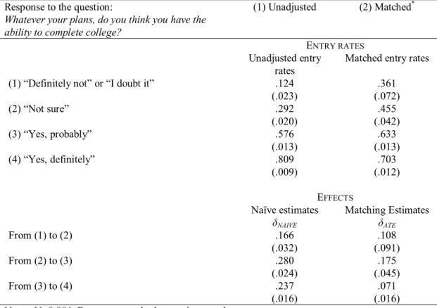
Table 1.1. Hypothetical Mapping Function Relating Educational Attainment to the Occupation it Will Result In. ... 26 Table 1.2. Standardized Bias Values for Black-white differences in Pretreatment Variables... 36 Table 1.3. The Proportion of Whites and Blacks Entering College... 38 Table 2.1. Variables Used to Analyze the Perceived Ability to Complete College. ... 62 Table 2.2. College Entry Rates for Students at Each Level of Perceived Ability to Complete College... 67 Table 2.3. Coefficients from Models Predicting Perceived Ability... 72 Table 3.1. Variables Used to Analyze Psychic Costs. ... 88 Table 3.2. Proportion of Students at Each Fourth of Psychic Costs Expecting a 4-year College Degree or Higher... 95 Table 3.3. Coefficients from Regression Models Predicting the Psychic Costs of Schooling. ... 97 Table 4.1. Variables Used to Analyze Occupational Preferences... 115 Table 4.2. Coefficients from Regressions Predicting the Characteristics of Occupations Wanted at Age 35... 133 Table 4.3. Odds-Ratios from Logistic Regressions Predicting the Expectation of a 4-year College Degree. ... 140 Table 4.4. Odds Ratios from Logistic Regressions Predicting Educational Expectations and College Entry... 146 Table 4.5. Regression Coefficients from Models Predicting Sheaf Variables for Job Values and Occupational Expectations. ... 150 Table 5.1. Variables Used to Analyze Beliefs About Educational Requirements of Expected Occupations. ... 166 Table 5.2. Proportion of Students at Each Perceived Educational Requirement Level Entering a 2- or 4-year College... 179 Table 5.3. Coefficients from Regressions Predicting the Educational Requirements of Occupations Wanted at Age 35... 188 Table 5.4. Regression Coefficients from Multilevel Models Predicting Education Beliefs... 190 Table 6.1. Actual and Counterfactual College Entry Rates for Respondents in Each Parental Education Group... 202 Table 6.2. Actual and Counterfactual College Entry Rates for Respondents in Each Cognitive Skill Fourth. ... 205 Table 6.3. Actual and Counterfactual College Entry Rates for Whites, Blacks, and Hispanics. ... 206 Table 6.4. Actual and Counterfactual College Entry Rates for Males and Females.. 207 Table B.1. Variables Used in the Analysis. NLSMY66... 221 Table C.1. Uniform Occupation Categories for the NELS88 and 2003 American Community Survey. ... 223 Table C.2. Uniform Education Categories for the NELS88 and 2003 American
CHAPTER 1. SUBJECTIVE RATIONALITY AND
POSTSECONDARY SCHOOLING DECISIONS
This dissertation attempts to answer the question “Why do some adolescents pursue college while others do not?” In attempting to answer this question my focus is on what I call “college-encouraging” preferences and perceptions, which are
preferences and perceptions that make adolescents more likely to pursue college. The model I develop engages the rational choice literature in both sociology and
economics, but it deals primarily with considerations outside the scope of traditional rational choice models. I consider nonpecuniary costs and benefits, and I focus on interpersonal variation in preferences and perceptions and how this variation affects college entry decisions.
In this introductory chapter I justify my theoretical approach, outline the methods I use, and provide a brief overview of the subsequent chapters.
WHY DO SOME PEOPLE GET MORE EDUCATION THAN OTHERS?
The relationship that postsecondary education has with a variety of outcomes makes it among the most important issues in the study of social inequality. Most commonly cited is the effect of postsecondary education on earnings. Estimation of the causal effects of schooling on earnings has proven surprisingly difficult, with ability bias and measurement error in self-reported schooling representing formidable obstacles to credible estimation. Despite these difficulties a near consensus has formed among labor economists that education pays handsomely at the individual level and is well worth the investment (Card 1999). Education appears to have beneficial effects on other labor-market outcomes including employment (versus unemployment) and working conditions (Jencks, Perman, and Rainwater 1988; Duncan 1976). Evidence
also suggests that postsecondary education affects a range of nonmarket outcomes including health, attitudes, and marriage duration (Wolfe and Zuvekas 1997; Kingston et al. 2003).
Largely because of its centrality in the development and maintenance of the stratification order, considerable effort has gone into understanding why some adolescents obtain more education than others. Research is conducted across most of the social sciences, but the most influential theoretical perspectives for understanding educational decisions have been developed in sociology and economics. Status attainment models—especially the “Wisconsin Model” of status attainment—have been highly influential in sociology (often as a foil). Investment models are dominant in economics. It is useful to begin with early formulations of the Wisconsin Model and investment models because their simplicity and familiarity provide a useful point of departure to introduce developments after their original formulations, including the themes I wish to develop.
THE “WISCONSIN MODEL” OF STATUS ATTAINMENT
Blau and Duncan (1967) formulated a basic model of intergenerational status attainment linking family background to occupational attainment. In it, educational attainment mediates the relationship between family background and adult
occupational attainment. Family background influences educational attainment, and educational attainment in turn influences occupational attainment.
A major development in the status attainment tradition occurred only two years later with the publication of Sewell, Haller, and Portes’s (1969) “Wisconsin Model” of status attainment, so named because a sample of Wisconsin high school seniors was used in the empirical analysis. The objective of the research was to postulate and empirically examine the role of social psychological constructs that linked exogenous
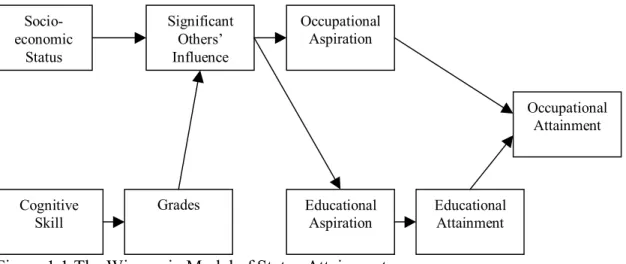
variables—family background and cognitive skill—to educational and occupational attainment. Figure 1.1 presents the path model describing the proposed causal
relationships among the variables. As Figure 1.1 shows, educational and occupational aspirations, which are assumed to represent underlying motivation, are the proximate causes of educational and occupational attainment. Based on social psychological findings showing the importance of others in the “definition of the situation” (e.g., Sherif 1935) and the influence of others’ expectations on one’s own aspirations, aspirations are assumed to be caused by the expectations of significant others, such as the expectations of parents, teachers, and peers. Significant others’ expectations are primarily caused by adolescents’ grades and family background. In theoretical elaborations significant others’ expectations influence adolescents’ educational aspirations through the combined forces of self-reflection, imitation, and adoption (Haller 1982), but focus has traditionally been on the most straightforward
socialization model in which adolescents simply adopt significant others’
expectations. Because aspirations are the proximate cause of attainment, it is proposed that manipulation of aspirations may influence later attainment.
Figure 1.1 The Wisconsin Model of Status Attainment.
Socio-economic Status Significant Others’ Influence Occupational Aspiration Educational Aspiration Grades Cognitive Skill Occupational Attainment Educational Attainment
Subsequent research questioned the omission of several paths, such as the path leading from mental ability to significant others’ influence (Sewell, Haller, and
Ohlendorf 1970). However, most evidence is consistent with the Wisconsin Model, and the original study has been replicated with numerous datasets that all reach the same basic conclusion that the effects specified in Figure 1.1 are all fairly strong.
INVESTMENT MODELS OF SCHOOLING DECISIONS
Human capital and signaling theory dominate theory and research on educational attainment in labor economics. Human capital consists of inalienable personal assets that can be rented out in the form of labor to result in an income stream in the form of wages. If a person chooses to increase their human capital they must make investments that allow them to rent out their labor at a higher wage. Education is seen as an investment made to increase human capital. Signaling theory assumes that productivity differences across educational attainment levels exist before schooling differences. For example, those with a college degree are on average more productive than those with high school diplomas, but schooling did not cause these differences. Schooling does affect earnings, however, because it provides probabilistic information about these unobservable, preexisting productivity differences to potential employers. For present purposes, the mechanism through which schooling affects earnings is unimportant. The essential point is that adolescents see schooling as an investment. Adolescents weigh the costs and benefits of schooling and their other alternatives (which could include labor market activity, leisure, domestic labor, criminal activity, and parenthood) and decide to continue their schooling if its net benefits are higher than those of their other alternatives. Schooling’s benefits are primarily conceived of as higher future wages, but nonpecuniary labor-market outcomes may be considered
as well. Schooling’s costs include direct costs (e.g., tuition, books), opportunity costs (i.e., forgone earnings), and “psychic costs” (e.g., the disutility of studying).
Evidence is generally consistent with predictions of investment models. An abundant literature on the causal effect of schooling on wages concludes that
postsecondary schooling increases earnings (for a review see Card 1999), and trends in enrollment and educational expectations in the 1970s and 1980s suggest that
adolescents respond to changes in the returns to education (Morgan 1998). Evidence also supports the importance of costs. Net direct costs, often defined as tuition minus financial aid, lower enrollment (for a review see Ehrenberg 2004). Less compelling evidence suggests that opportunity costs are important as well. Higher wages in local labor markets lower the probability of attending college (Venti and Wise 1983) as does a low rate of unemployment (Rivkin 1995). Psychic costs have generally been ignored except when they are inferred from behavior using the logic of “revealed preferences” (Lazear 1977; Cunha, Heckman, and Navarro 2006).
Some research has begun to look at adolescents’ perceptions of the costs and benefits of college because perceptions—not information at researchers’ disposal— should determine investment decisions. Avery and Kane (2004:382, Table 8.15) provide information from Boston-area high school students who estimated both tuition at several nearby colleges and the effect that a bachelor’s degree would have on their own earnings. Avery and Kane used this information in conjunction with assumptions about discount rates to calculate the implied present value of a bachelor’s degree for each student relative to working immediately after high school. They found that about 85 percent of students whose implied present value of a bachelor’s degree was positive (i.e., it was higher than the present value of working immediately after high school graduation) planned to obtain bachelor’s degrees. However, they also found that almost 70 percent of high school students whose implied present value was negative
planned to obtain a bachelor’s degree and that 95 percent of students from affluent neighborhoods whose implied present value was negative planned to obtain bachelor’s degrees. These findings led Avery and Kane to conclude that “subjective beliefs about the payoffs to college are only weakly related to students’ plans for college” (385). Rouse (2004) also provides evidence that higher perceived returns are only weakly related to college plans.
What about the perceived ability to finance college? Avery and Kane (2004) found that the more a student thought college would cost, the less likely they were to plan to attend; however, the relationship was very weak.1
SHORTCOMINGS OF THE WISCONSIN AND INVESTMENT MODELS
Theoretical and empirical shortcomings have prevented widespread acceptance of either the Wisconsin Model or investment models, including the many variations of these models that have been developed. Most important among these shortcomings have been conceptual issues raised by critics, inattention to structural forces in the educational attainment process, and the inability of the models to explain some puzzling empirical findings.
CONCEPTUAL ISSUES. A good deal of research framed explicitly within the status attainment tradition was conducted in the 1970s and early 1980s, but concerns about key constructs led to a sharp decline after this period. The emphasis on
aspirations and expectations was harshly criticized. Bourdieu (1973) questioned the claim that aspirations and expectations caused educational attainment and argued that expectations were largely statements of known probabilities that are determined by
1 Strangely, the more a student thought college would cost, the more likely they were to think that they
class background. Alexander and Cook (1979) convincingly showed that educational expectations do not always represent motivation. Using data on students surveyed in their senior year of high school, they found that some adolescents’ expectations were essentially extemporaneous responses representing no real commitment to the stated outcome. That expectations are not necessarily goals that adolescents strive for is also apparent in the absurdly high educational expectations that have been recorded, especially recently (e.g., Reynolds et al. 2006).
Furthermore, developers of the Wisconsin Model showed a concern for the effects of education on occupational attainment in their models, but their models assume that adolescents don’t share this concern. Labor-market goals play no role whatsoever in educational expectations or attainment, and the theory fails indicate why anyone would go to college to begin with. Even if the socialization story is accepted we do not really know why significant others might expect anyone to continue their education.
Rational choice theory has at times received a cool reception in sociology. Some argue that it is “masculinist” (England and Kilbourne 1990), not self-sufficient (i.e., it must be supplemented with other theories to explain all of what sociologists want to explain) (Wrong 1997), and not the domain of sociology its explanatory merits notwithstanding (Blau 1997). Investment models in economics have been developed largely within what I would call a “strict” rational choice framework, and the most common criticisms are leveled at the unrealistic assumptions that accompany strict rational choice models. The strictest variants make several logical assumptions about preferences, such as transitivity, which experiments reveal to often be false. More often criticized are the motivational and cognitive assumptions, such as the assumptions that actors seek to maximize their material self-interest and that they
possess all of the information and cognitive capacity necessary to select the course of action that maximizes their material self-interest.
STRUCTURAL FORCES. Both the Wisconsin Model and investment models have been criticized for ignoring structural factors that may operate as barriers to
educational attainment, such as grade retention and tracking. This line of criticism (e.g., Kerckhoff 1976) led to research focusing on the structure of schools and the allocation of students to different positions within this structure. A large and growing body of “school effects” literature seeks to understand how different schools affect students differently (Sørensen and Morgan 2000).
Research taking this “structural perspective,” as I term it, shows the importance of structural factors. Those in the academic track (also known as the college preparatory track) in high school appear to experience greater gains in
cognitive skill than those in the general or vocational track (Gamoran and Mare 1989) and are much more likely to attend four-year colleges. Most of the literature suggests that the net effect of grade retention is harmful because it leads to higher dropout rates, but its role as a motivation for achievement is questionable (Hauser 2004).
The so-called “Coleman Report” (1966) concluded that school resources have small effects on learning. Since the Coleman Report, numerous studies have
confirmed that some factors—such as homework, graduation requirements, and discipline—that one might assume would affect learning also have little or no effect (Chubb and Moe 1990). Other studies have shown that some school characteristics are important for some outcomes. Coleman and associates found that more learning occurs in Catholic schools (Coleman, Hoffer, and Kilgore 1982), perhaps because Catholic schools have a larger percentage of students in college preparatory tracks. Characteristics of schools, such as their racial-ethnic mix, have been found to affect a
range of outcomes such as dropout rates and aspirations (Goldsmith 2004). Some research points to the importance of school size. Wicker (1969) found that students in small high schools participated more and felt they were serving important roles. Others argue that small school size creates an inviting atmosphere (Meier 1995; Morgan and Alwin 1980).
UNEXPLAINED EMPIRICAL FINDINGS. Another line of criticism concerns empirical findings that neither the Wisconsin Model nor investment models have explained satisfactorily. Most troubling have been findings of minority-white
differences in the educational attainment process. Conditional on family background and cognitive skill, blacks’ (Morgan 1996; Hout and Morgan 1975; Bennett and Xie 2003) and Asians’ (Goyette and Xie 1999) college plans, enrollment, and attainment are higher than those of whites’ plans, enrollment, and attainment. Results are not as well documented for Hispanic-white differences, but the weight of the evidence
suggests that Hispanics’ conditional plans and attainment are higher than whites’ plans and attainment as well (Kao and Tienda 1998).
Because the Wisconsin Model specifies that aspirations and attainment are ultimately determined by family background and cognitive skill, it cannot account for the high expectations and attainment of minorities that exist conditional on these factors. Investment models—at least traditional models that focus narrowly on pecuniary costs and benefits—have also been unable to explain minority-white differences. The evidence suggests that education has roughly the same returns for blacks, whites, and Hispanics (Barrow and Rouse 2006; Ashenfelter and Rouse 2000) and that blacks, whites, and Hispanics have roughly the same perceptions of the costs and benefits of postsecondary education (Avery and Kane 2004).
Alongside enduring minority-white differences, a new group difference puzzle has developed. The educational expectations and attainment of females have
historically been below those of males, but a long-term, strong, upward trend has led to females having higher expectations and attainment than males (National Center for Education Statistics 2006:159; Buchmann and DiPrete 2006).2 The secular trend in females’ expectations relative to males is unsurprising given the rise of female labor force participation, but the Wisconsin Model cannot explain higher expectations and attainment among females because males and females have essentially identical test scores and family resources. Investment models also poorly explain sex differences because—although there is some evidence of higher returns for females (Jacob 2002; DiPrete and Buchman 2006)—education appears to have roughly the same return for males and females.
I also argue that the Wisconsin Model and investment models provide unsatisfactory accounts of the effects of cognitive skill and family background on educational attainment. The Wisconsin Model specifies that cognitive skill affects grades, which affect significant others’ expectations, which affect students’ attainment (see Figure 1.1). However, a fairly strong relationship between cognitive skill and educational attainment remains net of both grades and significant others’ expectations. Human capital oriented researchers often suggest that cognitive skill increases
schooling’s returns (e.g., Frank 1985:211; Herrnstein and Murray 1994) or lowers schooling’s psychic costs (Cunha, Heckman, and Navarro 2006; Garen 1985), but these claims have not been empirically demonstrated.
Despite the centrality of family background in the Wisconsin Model, it is never clearly spelled out why significant others of those with advantaged family
2 This net-female advantage is now so great that some administrators are considering “affirmative
action” admission policies for male applicants (Green and Green 2004, cited in Buchmann and DePrite 2006).
backgrounds have high educational expectations. Family income should be related to the ability to comfortably finance college (or finance it at all), but other measures of family background have strong relationships with educational attainment conditional on family income. Most notably, estimation always suggests that parents’ education has a large effect on adolescent educational attainment conditional on family finances and other predictors of educational attainment. It is sometimes vaguely suggested that well-educated parents value the cultural or symbolic benefits of college (Raftery and Hout 1993; Boudon 1974; Ellwood and Kane 2000), but this has not been shown. Returns to education do not seem to vary systematically with family background (Altonji and Dunn 1996), which leaves traditional investment models unable to explain family background effects that exist conditional on the ability to finance college.
SUBJECTIVE RATIONALITY AND SCHOOLING DECISIONS
I propose a synthetic framework focusing on college entry and drawing on what I perceive to be the strengths of the Wisconsin Model and investment models. My explanatory framework adopts the basic structure and explanatory agenda of the Wisconsin Model. In the Wisconsin Model, interpersonal variation in educational attainment is explained by interpersonal variation in social psychological constructs, namely aspirations. My approach also posits that interpersonal variation in social psychological constructs causes variation in educational outcomes, but in my model these psychological constructs are preferences and perceptions rather than aspirations.
While drawing on the status attainment tradition, my approach could fairly be characterized as rational choice theory because adolescents are ultimately seen as making their schooling decisions in a purposive, goal-oriented manner. I pursue a rational choice strategy because, although other forces doubtlessly come into play, this
is exactly where we should expect people to think somewhat strategically: college entry is a major decision involving potentially large costs and benefits.
I mentioned earlier that rational choice theory has received at times a cool reception in sociology. Before laying out more of the specifics of my approach it is useful to defend at the outset against common criticisms of rational choice
perspectives because doing so helps position my approach in broader debates in the literature.
Some criticize the unrealistic assumption of rational choice models, such as the assumption that actors possess complete information, act only in their self-interest, care only about material well-being, and so on. Rational choice theory is now considered more a “family of theories” (Hechter and Kanazawa 1997) than a single theory with a single set of assumptions. Several approaches, such as “bounded rationality” (Simon 1982), “subjective rationality” (Boudon 1989), and inclusive or “thick” modeling (Mansbridge 1990) have been offered as more realistic alternatives. The approach I offer is firmly within this “realistic tradition.”3
Yet some sociologists object even to these more realistic models because rational choice has no place in sociology (e.g., Blau 1997). I concur with Goldthorpe’s (2007:166) position that such sociologists “take an unduly partial view of what
constitutes the sociological tradition” because the means-ends logic of rational choice theory represents a major portion of the work that mainstream sociologists engage in, including work performed by rational choice theory’s detractors (Heckathorn 1997; Hechter and Kanazawa 1997).
3 I find the arguments against rational choice theory generally unpersuasive and often unreasonable, but
I note that uncharitable critiques run in both directions. When rational choice proponents criticize “over-socialized” actor models they characterize these models in ways that I think only a small minority of advocates of socialization models would accept as realistic. Just as rational choice researchers emphasize rationality without thinking that actors are thoroughly rational, I suspect that socialization-oriented researchers emphasize socialization without thinking that actors never make decisions.
Some important sociological traditions do downplay the role of subjectivity.4 But at the same time, a major current in sociology has always been the importance of subjectivity, and sociology has long stressed the importance of beliefs, perceptions, social constructions, the “definition of the situation,” and related concepts on the supposition that subjectivity is crucial to understanding human behavior (Weber 1978; Thomas 1923; Mead 1934). Indeed, subjectively rational action is emphasized in Weber’s well-known “types of social action” framework (Weber 1978:24–26) as the most promising route to understanding social behavior. The rational choice approach taken here could fairly be called an interpretive approach in the spirit of Weber’s sociology because it calls for beginning the analysis by understanding others’ way of seeing the world—or in this case their way of seeing a particular decision—and then determining how their perspective affects their behavior.5, 6
I argue that rational choice research in education has concentrated too much on models without empirical content and that more empirical analysis is needed.
However, my first step is to discuss in abstraction aspects of schooling decisions to develop a model that I believe captures much of adolescents’ thinking when making these decisions. I build this model using utility functions. This is not strictly necessary, but utility functions provide a useful framework for the unambiguous communication of ideas. I begin with a traditional investment framework representative of the most
4 For example, the Marxian tradition downplays consciously held beliefs on the assumption they are
“epiphenomena” that do not themselves motivate or explain behavior. Important pieces of Durkheim’s work also argue against appeals to the thought processes of individuals. Most famously, Durkeim warns that “Every time that a social phenomenon is directly explained by a psychological phenomenon, we may be sure that the explanation is false” (Durkheim 1966:104). He does not mean to exclude psychology and he did some backtracking in subsequent editions of the Rules of the Sociological Method. Nonetheless, Durkheim certainly downplayed individuals’ subjectivity as a cause of behavior.
5 My perspective is also in the spirit of Weber’s types of social action schema in that—while I focus
narrowly on rational action for the research at hand—I do not believe that all social action is rational. I believe that social action can sometimes be more fairly characterized as nonrational and oftentimes be more realistically characterized as a blend of the various ideal types of social action that Weber describes. The approach I offer is a one-sided exaggeration that focuses on a certain group of factors.
6 In this spirit, Kiser and Hechter (1998:798) have referred to a variant of rational choice theory as
basic investment models to provide a clear and explicit system through which I introduce changes. I do so by relaxing and changing the assumptions to arrive at the flexible model I take as my empirical point of departure. The model is not
parsimonious by most standards, and much of the framework has already been
outlined by others (Morgan 2005; Breen and Goldthorpe 1997; Xie and Goyette 2003), it must be granted. What is valuable is that the model outlines an empirically testable agenda.
BASIC INVESTMENT MODEL. Taking only four-year colleges into
consideration, in a basic investment framework students should enroll in college if:
(
BBA−CBA) (
> BHS −CHS)
Where BBA are the benefits of a bachelor’s degree, CBA are the costs of a bachelor’s degree, BHS are the benefits of a high school diploma, CHS are the costs of a high school diploma, and all costs and benefits are pecuniary in nature.
UTILITY FUNCTIONS. Many models equate earnings with utility; doubling earnings doubles utility, tripling earnings triples utility, and so on. In all probability, however, earnings has diminishing utility; doubling earnings, for example, will increase utility but it will less than double it. This point is important in understanding choice under conditions of uncertainty where people are often found to be risk-averse (von Neumann and Morgenstern 1944). Regardless of the exact function, the notion here is that utility is a function of earnings and not necessarily a linear function.
Now the costs and benefits are the arguments of utility functions, and the decision rule is enroll if:
) ( ) (BBA CBA U BHS CHS U − > − Or equivalently: ) ( ) ( ) ( ) (BBA U CBA U BHS U CHS U − > −
INVESTMENT WITH UNCERTAINTY. Comay, Melnik, and Pollatschek (1973) were the first to systematically treat postsecondary education decisions as choice under conditions of uncertainty and incorporate the probability of completing an educational stage into the decision of whether or not to commence that stage. An adolescent may not know, for example, if their current work habits are sufficient for graduation or if they can substantially improve them if they are not. This is important in the decision to pursue a postsecondary degree because labor market outcomes are contingent on the acquisition of educational credentials (Kane and Rouse 1995; Faia 1981), and most adolescents probably know this. Consequently, the decision of whether or not to enter college depends on the probability of graduation. Following convention, the probability of graduation is denoted π. Now the decision rule is enroll if:
(
U(BBA)−U(CBA))
+(1−π)(
U(BSC)−U(CSC)) (
> U(BHS)−U(CHS))
πWhere the subscript SC stands for “Some College” and indicates that the adolescent entered college but did not graduate. The meaning of “Some college” can range from withdrawing immediately after enrollment to withdrawing immediately before graduation, but for my purposes these differences are unimportant.
NONPECUNIARY COSTS AND BENEFITS. We know surprisingly little about what motivates investments in postsecondary education. Despite the decades old tradition of treating education as an investment made to improve earnings, there is little direct evidence that earnings in particular motivate noncompulsory schooling. The basic argument, generally unstated, is simply: everybody wants high earnings; schooling appears to increase earnings; therefore, people go to school to increase their earnings.
The only real supporting evidence is that trends in returns are followed by trends in college enrollment (Ehrenberg and Smith 2000:301–302) and educational expectations (Morgan 1998). It is worthwhile to examine these trends because those who have offered them as evidence have ignored alternative nonpecuniary
explanations. Figure 1.2A presents trends in the proportion of 18 to 24 year olds enrolled in college for the years 1968 to 1999 and trends in the “college earnings premium,” which is the ratio of the earnings of those with bachelor’s degrees and the earnings of those with high school diplomas. The college premium declined in the early 1970s and has increased steadily beginning around 1980. Enrollment in college appears to have tracked this trend, especially from 1980 onwards. However, female enrollment in college has been increasing steadily for decades, likely as a result of changing gender role attitudes and changes in the role females play in the labor market. Figure 1.2B shows that among females trends in college earnings premiums and college enrollment do not track one another well and that female college
enrollment was increasing through the period of declining college premiums from 1975 to 1980. Figure 1.2C shows the trends for males, which do seem to follow one another somewhat closely.
Just as a college premium can be generated for earnings, college premiums can also be generated for nonpecuniary labor-market outcomes. Ratios of some
point, but the difficulties can be ignored to generate some simple trends.7 Figure 1.3 shows the percentage of 18 to 24 year old males enrolled in college and college premiums for six nonpecuniary labor-market outcomes measured using characteristics of the occupations respondents report. Occupational characteristics are taken from O*NET98. The O*NET98 data and variables will be described in greater detail in Chapter 4, but self-explanatory variable names should be sufficient for now. Just as Figure 1.2C showed that the college earnings premium could have caused the increase in male college enrollment, especially beginning around 1980, Figure 1.3 shows that college premiums in nonpecuniary outcomes could also have caused the increase. Specifically, Figure 1.3 shows that college premiums in job security, occupational status, work that satisfies “Investigative interests” (such as abstract problem solving), and work that involves decision-making and ability utilization (the use of one’s skills) have all followed roughly the same trends as college enrollment.
Figure 1.3 also shows that the college premium increased for deductive reasoning requirements as well. Deductive reasoning requirements are not normally thought of as desirable nonpecuniary benefits, but they probably are sought after by many people. The trend in deductive reasoning requirements illustrates the more general trend that anything strongly related to cognitive skill (such as Investigative interests, occupational prestige, and so on) shows the same basic trend as college enrollment. (This is not true for females, but other factors were probably driving female trends in enrollment.)
It is unclear whether the trends in Figures 1.2 and 1.3 should be interpreted as evidence of pecuniary motives or nonpecuniary motives, but the broader evidence that nonpecuniary job characteristics are important is unequivocal. Studies find that job
7 A less problematic approach would be to estimate changes in the effect of education as changes in the differences in nonpecuniary outcomes between those with bachelor’s degrees and high school diplomas. Results based on differences yield nearly identical results.
satisfaction is only weakly affected by earnings (Gruenberg 1980). Research on compensating differentials shows that workers will forgo higher earnings for more pleasant and safer jobs. Jencks, Perman, and Rainwater (1988) developed an “Index of Job Desirability” using the rankings people gave of their own jobs in conjunction with their descriptions of their own jobs. While they found that earnings were the single strongest determinant of a job’s desirability, other factors (such as autonomy, full-time employment, vacation time, on-the-job training, job security, variety, cleanliness, and unionization) were collectively twice as important as earnings. People care about having an interesting job, a safe job, a respectable job, and so on (Jencks, Perman, and Rainwater 1988; Johnson and Elder 2002), and it is reasonable to think that
adolescents go to school to obtain these outcomes. Permitting nonpecuniary costs and benefits, the decision rule is enroll if:
(
U(BBA•j)−U(CBA•j))
+(1−π)(
U(BSC•j)−U(CSC•j)) (
> U(BHS•j)−U(CHS•j))
π
Now costs and benefits are indexed by j, which indicates that multiple types of costs and benefits—pecuniary and nonpecuniary—are permitted.
HETEROGENEOUS UTILITY FUNCTIONS. Thus far preferences have been assumed to be homogeneous across adolescents, which is not uncommon in rational choice models. This is one point at which investment models and the Wisconsin Model have diverged sharply. In the Wisconsin Model adolescents have different goals. Some adolescents want to go to college and others do not; some adolescents want to be plumbers and others want to be engineers. These differences in aspirations and expectations drive differences in attainment. In contrast, many investment models assume that all adolescents possess identical preferences or permit preferences to vary
interpersonally but infer them after-the-fact from behavior (e.g., random utility models) rather than measuring them before analysis for their predictive value.
Utility functions need not be the same for everyone. Surely most people want high earnings, but the subjective value of earnings just as surely varies from person to person. If education is believed to increase earnings, then a “preference for earnings” could increase the utility of schooling. The literature on job values, which is reviewed in Chapter 4, supports the notion that interpersonal differences in the conversion of earnings into utility are both considerable and directly measurable. These differences in preferences also appear to have consequences; for example, Long (1995) shows that self-reports of the importance of financial success predict annual income conditional on a range of covariates.
Of course adolescents also vary in their preferences for nonpecuniary outcomes and these too may affect postsecondary schooling decisions. Now the decision rule is enroll if:
(
Ui(BBA•j)−Ui(CBA•j))
+(1−π)(
Ui(BSC•j)−Ui(CSC•j)) (
> Ui(BHS•j)−Ui(CHS•j))
π
Where the subscript i has been added to indicate that preferences are allowed to vary interpersonally across adolescents.
Permitting heterogeneous utility functions deserves special attention because many rational choice proponents strongly object to it. Surprising though it may seem, there are those who have argued that utility functions are essentially invariant
interpersonally (Becker and Stigler 1977; Becker 1976; Freidman 1953). Most rational choice proponents do concede that preferences vary interpersonally, but they caution against making models more realistic by permitting preferences to vary because the cure is worse than the disease. Allowing interpersonal variations in preferences, it is
1. 5 1. 6 1. 7 1. 8 Co lle ge Pr em iu m 25 30 35 % in C o llege 1970 1975 1980 1985 1990 1995 2000 Year % in College College Premium
A. Males and Females
1. 7 1. 8 1. 9 2 2. 1 Co lleg e Pr em iu m 20 25 30 35 40 % i n C o llege 1970 1975 1980 1985 1990 1995 2000 Year % in College College Premium B. Females 1. 2 1. 3 1. 4 1. 5 1. 6 1. 7 C o llege Pr e m iu m 26 28 30 32 34 % i n Co lle g e 1970 1975 1980 1985 1990 1995 2000 Year % in College College Premium C. Males
Figure 1.2. Trends in College Enrollment among 18–24 Year-Olds and the College Earnings Premium. CPS 1968–1999.
Notes. Enrollment data are from the October CPS. Earnings data are from the March CPS. Trends are three-year moving averages.
1. 38 1. 4 1. 42 1. 44 1. 46 O ccupa tional P re st ige 26 28 30 32 34 % in C o llege 1970 1975 1980 1985 1990 1995 2000 Year % in College Occ. Prestige 1. 35 1. 4 1. 45 1. 5 In ve st ig a tiv e I n te re st 26 28 30 32 34 % in C o llege 1970 1975 1980 1985 1990 1995 2000 Year % in College Investigative 1. 54 1. 56 1. 58 1. 6 1. 62 D e ci si on ma ki ng 26 28 30 32 34 % in C o lle g e 1970 1975 1980 1985 1990 1995 2000 Year % in College Decisionmaking 1. 25 1. 26 1. 27 1. 28 1. 29 1. 3 A b ilit y U til iz a tio n 26 28 30 32 34 % in C o lle g e 1970 1975 1980 1985 1990 1995 2000 Year % in College Ability Util. 1. 08 1. 09 1. 1 1. 11 1. 12 Se cu rity 26 28 30 32 34 % in C o lle g e 1970 1975 1980 1985 1990 1995 2000 Year % in College Security 1. 3 1. 32 1. 34 1. 36 1. 38 1. 4 R eason in g 26 28 30 32 34 % in C o lle g e 1970 1975 1980 1985 1990 1995 2000 Year % in College Reasoning
Figure 1.3. Trends in Male College Enrollment and Trends in Possible Incentives for College Enrollment. March CPS 1971–1999.
Notes. Enrollment data are from the October CPS. Earning data are from the March CPS. Trends are three-year moving averages. See text (the section titled Data) for details on the occupational
argued, destroys the predictive value of rational choice models. For example, if someone decided not to go to college and I simply asserted “They must not like school” then critics would object that “preferences can explain everything, therefore they explain nothing.” I think this is not a criticism of preferences at all. It is a criticism of post-hoc explanations based upon no data. It should be just as
objectionable if I claimed without evidence that “Their net pecuniary gain must be low.” The problem is dealt with by measuring preferences not by precluding the use of preferences because they seem common in post-hoc explanations.8
A second criticism is that troubling measurement issues cast doubt on the validity of self-reported preferences (Hechter 1992; Fischhoff 1991). Therefore, even when preferences are measured, it is argued, they often should not be used by
researchers. Measuring preferences is difficult, but so is measuring any concept with self-reports. If we excluded all variables with considerable measurement error we would have to exclude a great many variables indeed. Included among them, I would imagine, would be many of the variables used with rational choice models that assume homogeneous utility functions. If preferences are measured as poorly as many suggest then they should have no predictive power, but this has not been shown. The value of measured preferences should be examined rather than dismissed before empirical inquiry.
I argue that self-reported preferences are valuable, but I concede that unconscious mechanisms sometimes shape self-reported preferences in such a way that they appear to have explanatory power when they in fact do not. Consider the case of interpersonal differences in preferences for different occupations. Someone who
8 Based on my own reading of the literature I would add that the explanations based on unmeasured
preferences that some criticize so harshly are rare, and explanations invoking interpersonal differences in preferences are typically made on the basis of some evidence or are merely presented as possibilities. Appeals to unmeasured costs are probably just as common.
initially wanted to become a physician may realize that they lack the ability or
motivation to complete the training required to meet this goal. They may subsequently disparage the goal and argue that becoming a physician is actually an undesirable outcome that they do not want for themselves. This is the theory of adaptive
preference formation of Rokeach (1973) or the “sour grapes” mechanism discussed by Elster (1983) in which values change to preserve a positive self-concept. I take this mechanism seriously and attempt to address it where I can. I generally cannot address it in a completely satisfactory manner, but I do discuss the direction of bias that would be expected if the sour grapes mechanism was operating.
Critics of “heterogeneous preferences” explanations also claim that the cure is worse than the disease because the disease is not as bad as it seems. Hechter (1994) distinguishes between “immanent values” and instrumental values.” Immanent values are commodities that rational actors derive utility from. Instrumental values are the commodities that rational actors use to produce immanent values. Hechter argues that it is reasonable to assume that instrumental values (e.g., money) are important to everyone because they can be used in the pursuit of immanent values, including altruism. Conversely, the importance of many immanent values should be randomly distributed. Therefore, while they may be essential to understanding an individual’s behavior, they will be unimportant in understanding the behavior of aggregates because they will tend to cancel out leaving group behavior explained strictly with instrumental values. This is the defense of the so-called “typical values” assumption: only those values that are typical in the population will predict the behavior of aggregates.
The argument that almost all people value money seems quite sensible to me, and it may be productive to make this assumption in many situations. I argue that college entry decisions are not one of those situations. I seek to understand why some
individuals enter college and others do not, and I need interpersonal variation in something to explain interpersonal variation in college entry. For reasons of their own, economists have traditionally focused on interpersonal variation in budget constraints and pecuniary costs and benefits, but these seem unable to explain a considerable portion of interpersonal differences in schooling decisions. We know that immanent values differ—both in kind and in intensity—and there is every possibility that these differences affect schooling decisions. Perhaps interpersonal variation in preferences can be ignored when trying to predict the effect of tuition changes on enrollment but not when trying to understand why some adolescents enter college and others do not.
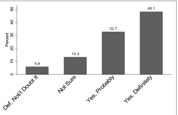
PERCEPTIONS ARE PERMITTED. As discussed, traditional rational choice models typically assume complete information, but this assumption is dropped with increasing regularity in the literature (e.g., Morgan 2005; Rouse 2004; Dominitz and Manski 1996; Avery and Kane 2004; Wilson, Wolfe, and Haveman 2005). It is dropped here, and decisions are assumed to be based on perceptions (or equivalently on beliefs). For example, I look at students’ perceptions of their ability to complete college rather than at more objective measures, such as grades, test scores, and so on. No notation is introduced to designate that perceptions are permitted, and it is to be understood that all costs and benefits are perceived.
In the college context much cannot be known with certainty because it is in the future. There is no way for an adolescent to determine, for example, what the returns to education will be over the course of their career, what their actual probability of future college completion is, and so on. Strictly speaking the distinction made here is not between perceptions and facts but between “rational forecasts” and “irrational forecasts.” Rational forecasts are reasoned predictions of future outcomes based on available evidence about the past and present. Irrational forecasts ignore available
evidence or use it unwisely. Irrational forecasts are permitted here, and they are an important part of the empirical analyses.
SATISFICING BEHAVIOR. Sometimes the effect that perceptions have on college entry is straightforward. For example, higher perceived ability to complete college should increase the probability of college entry and higher perceived psychic costs should lower the probability of college entry. It seems almost universally to have been assumed that perceptions of the effect of education on labor-market outcomes are another straightforward case, and that adolescents who believe that postsecondary schooling’s effects are high should be more likely to pursue postsecondary education because they are more apt to conclude that its benefits outweigh its costs (Becker 1993; Gambetta 1987; Morgan 2005).
This conclusion is based on the assumption that adolescents are maximizers or that they act like maximizers (such as would be the case if nonmaximizers imitated maximizers). Herbert Simon (1957) suggests that across a range of contexts actors are
satisficers rather than maximizers, by which he meant that they set goals and devise and pursue strategies to meet them. Satisficers are satisfied if their goals are met even if maximization has not been achieved or if it is not known if maximization has been achieved.
I propose that satisficing models apply to schooling decisions. Adolescents form labor-market goals based on their preferences and then make postsecondary schooling decisions with the objective of meeting these goals. I propose that, in Simon’s (1955) language, adolescents have mental mapping functions that relate educational attainment to occupational attainment. For example, an adolescent may perceive the mapping function presented in Table 1.1, which shows an adolescent who believes that with a high school diploma they can become a hospital orderly, with a
bachelor’s degree they can become a registered nurse working in a hospital, and so on. Table 1.1 uses occupations, but it is possible to also think of adolescents’ beliefs about more general occupational characteristics—such as earnings, authority, prestige, and so on—obtainable at different education levels. The approach taken here assumes that adolescents select an occupational goal and subsequently select educational attainment levels that will allow them to reach their occupational goals.
Table 1.1. Hypothetical Mapping Function Relating Educational Attainment to the Occupation it will Result In.
Educational Attainment Occupational Attainment High school dropout → Hospital custodian High school graduate → Hospital orderly
Some college → Practical Nurse
Bachelor’s degree → Registered Nurse in a hospital Master’s degree → Head Nurse at a hospital
PhD → Medical Researcher
Professional degree → Physician
While this way of modeling decisions seems sensible and realistic to many people, critics would object that it is not sensible to select an occupational goal without consideration of the schooling costs it entails. They would argue instead that educational and occupational goals develop simultaneously and that occupational goals are influenced by the type and amount of education an adolescent is willing to obtain. For example, an adolescent may ideally want to become a physician but may decide to set a different goal when they realize how much education is required for this occupation.
Furthermore, critics could object that the introduction of a satisficing model jeopardizes the logical coherence of my entire undertaking. The model is initially developed within a utility maximization framework, but then a satisficing decision rule is added. This is not an issue of doctrinal purity alone because it could be argued that if adolescents really are satisficers then the psychic costs of schooling should be
irrelevant to schooling decisions because occupational expectations must be met at all costs. As I have framed the decision, if an adolescent has decided that they want to become a registered nurse then nothing will stop them, including very high psychic costs of schooling and very low probabilities of college completion. This argument correctly accuses me of accusing adolescents of a degree of logical inconsistency. However, the empirical results presented in Chapter 2 through 5 support a model that blends utility maximizing and satisficing because they show that the perceived ability to complete college does increase the probability of entering college, the psychic costs of schooling do lower the expectation that college will be entered, and higher
perceived education requirements do increase the probability of college entry.
SOURCES OF PREFERENCES AND PERCEPTIONS. The proximate causes of college entry are my primary interest, but I also engage in analyses that attempt to locate the sources of college-encouraging preferences and perceptions. These analyses focus on family background, cognitive skill, gender, and race and ethnicity. I also address the role of the structure of schools and the placement of adolescents in different schools.
ESTIMATING CAUSAL EFFECTS
Much of the empirical analysis in subsequent chapters involves estimating causal effects, such as the effect of the perceived ability to complete college on college entry, and matching estimators are used to estimate many of the effects. The logic and virtues of matching estimators are best expressed in the language and concepts of the counterfactual model of causality. I do not present a complete overview of the counterfactual model, which can be found elsewhere (Morgan and Winship 2007).
Instead, the presentation is stylized to convey my own understanding of the logic and value of matching estimators.
Consider estimating the causal effect of a binary variable D on an outcome variable Y. Individuals are either exposed to the causal variable (D=1) or are not exposed to it (D=0). Adopting the language of experiments, in the counterfactual model respondents who are exposed to the causal variable are said to be exposed to the “treatment” and belong to the treatment group; those not exposed to the causal
variable are said to be in the control group and are called “the controls.”
Suppose that the data on the relationship between D and Y were generated in an experiment using random treatment assignment. The average treatment effect of D
on Y, which is denoted δ, could be estimated as the difference between the expected values of the outcome of the treatment and control groups:
] 0 | [ ] 1 | [ = − = = EY D E Y D δ
Suppose now that the data are from an “observational study” in which data has been generated by something other than a randomized experiment, such as a survey. One obvious way to estimate the average treatment effect is with the same estimator used in experimental studies. When used with observational studies this estimator is often called the naïve estimator:
] 0 | [ ] 1 | [ = − = =EY D E Y D NAIVE δ
In observational studies the naïve estimator is subject to two potential sources of bias. First, naïve estimators ignore possible initial differences between the treatment and control groups on “pretreatment” variables that may affect the outcome. Morgan
and Winship (2007) refer to the bias that these initial differences cause as baseline bias. Second, naïve estimators ignore the possibility that D affects members of the treatment group differently than it affects members of the control group. Morgan and Winship (2007:46) call this differential treatment effect bias. If the treatment and control groups differed on neither baseline values nor on the effect of the treatment we would be unconcerned with these biases, and we could use the naïve estimator to produce unbiased estimates of the average treatment effect of the treatment D.
To avoid these two sources of bias, ideally we would observe the expected value of the outcome Y of the treatment group under the control state; in other words, we would like to know what the outcomes of the treatment group would have been if it had not received the treatment. This is a counterfactual or potential outcome that we cannot observe and does not actually exist. In the counterfactual model it is useful to conceive of such an average counterfactual outcome, which is denoted as:
] 1 | [Y0 D=
E
Where the superscript “0” on the outcome Y indicates the control state. If we had this value, we could then estimate the average treatment effect for the treated:
] 1 | [ ] 1 | [ 1 = − 0 = =E Y D E Y D ATT δ
Where the superscript “1” on Y indicates the treatment state. The subscript ATT on the treatment effect signifies that we are estimating the average treatment effect for the treated, which is commonly abbreviated as ATT. This notation is necessary because differential treatment effects permit the possibility that the treatment effect for the treated differs from the treatment effect for the controls and
necessitates that researchers specify which causal effect they seek to estimate.9 I focus
on the ATT in this overview because it facilitates the introduction of key concepts and terminology.
According to two of its proponents in sociology the counterfactual model is “valuable precisely because it helps researchers to stipulate assumptions, evaluate alternative data analysis techniques, and think carefully about the process of causal exposure” (Morgan and Winship 2007:7). From my perspective the counterfactual model is valuable because it makes researchers think carefully about who should be compared to whom to estimate a particular causal effect. I cannot compare the treated under the treatment state to the treated under the control state because the latter data do not exist. I thus seek a control group that I believe is a good stand-in for the
treatment group in the control state. Specifically, I want a control group with the same expected value of the outcome that the treatment group would have in the control state. The principle aim of matching algorithms is the construction of control groups against which the treatment group can reasonably be compared to estimate the causal effect of D on Y.
When matching to estimate the ATT, observations in the control group are matched to observations in the treatment group on pretreatment variables believed to be important both in selection into the treatment and in determining the outcome. For each member of the treatment group, we search the control group for a person who has the same values for all of the pretreatment variables. In exact matching, cases that have no match are excluded from the analysis. More commonly some sort of a
“nearest neighbor” algorithm, such as Mahalanobis matching or “calipers” (Althuauser
9 As later chapters discuss, it is often difficult to decide which causal effect should be estimated.
Nonetheless, it is better to realize that a multiplicity of causal effects exists and to sometimes make a questionable decision which effect to estimate than to always estimate a causal effect with no concrete meaning as has long been the common practice when modeling the outcome with regression.
and Rubin 1971) can be used to allow imperfect matches but ensure that matches are close. However, when the number of variables on which the match is to be made increases, satisfactory matches can become unlikely even when imperfect matches are allowed. The result is that many observations in the treatment group must be excluded from the analyses.
In their seminal article, Rosenbaum and Rubin (1983) proposed that matches could be made on a scalar summary of the covariates—the propensity score—instead of on the matching variables themselves. Again, imperfect matches are typically allowed. True propensity scores are unavailable in observational studies, but they can be estimated based on observed variables and an appropriate model of the treatment selection process, such as a logit or probit model, that predicts selection into the treatment group with the pretreatment variables.
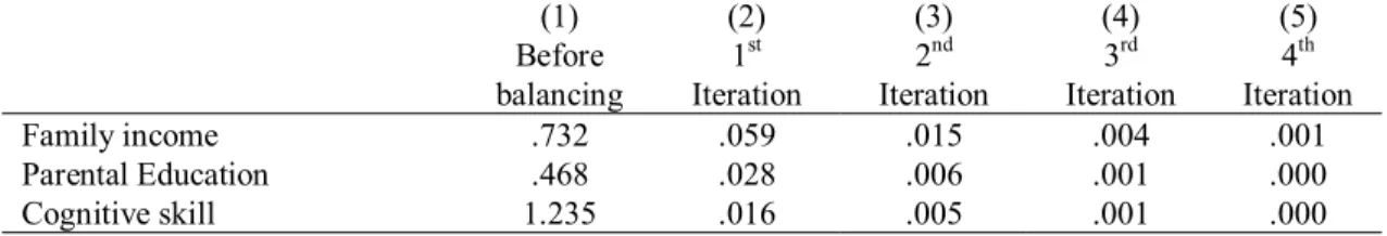
Rather than trying to match each person in the treatment group to a particularly similar person from the control group, in propensity score matching the goal is to “balance” the samples on the pretreatment variables. Samples are said to be balanced when they have the same distributions of pretreatment variables. This is different than finding a perfect or near-perfect match for each member of the treatment group. Pairs of observations matched on propensity scores may not be particularly similar on the pretreatment variables because the same propensity score can arise from different combinations of values for the pretreatment variables. Indeed, the reason we use propensity scores is that we often cannot match individuals on the covariates. Thus, propensity score matching is much like randomization in experiments where the goal is to have similar control and treatment groups, not to have pairs of identical people split into treatment and control groups.
Balancing addresses baseline bias by ensuring that the treatment group is compared to a control group with the same baseline values on important pretreatment
variables. What about differential treatment effect bias? The balancing process is believed to deal with differential treatment effect bias as well because causal effect size is likely related to pretreatment variables. For example, the effect that education has on earnings may be related to cognitive skill, so Cunha, Heckman, and Navarro (2006) estimated the effect of education on earnings separately for those who completed college and those who did not because these two groups have somewhat different distributions of cognitive skill.
Many matching algorithms exist (see Morgan and Winship 2007:107–109). Morgan and Harding (2006) show that these various matching estimators can be thought of and generalized as weighting estimators, in which the matching algorithm generates a set of weights for the control group that makes the control group similar to the treatment group on the pretreatment variables. For example, in exact or nearest neighbor matching without replacement, observations from the control group that are matched to observations in the treatment group are given a weight of one; observations that are not matched to cases in the treatment group are given a weight of zero. In exact or nearest neighbor matching with replacement, observations from the control group are given weights according to how many times they are matched to
observations in the treatment group.
I favor presentation and discussion using the logic of weighting because I think in terms of weighting, and working within a weighting framework facilitates
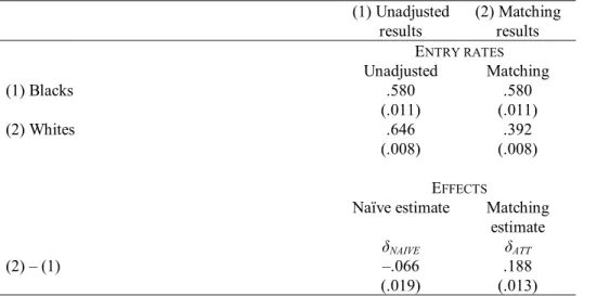
introduction of an innovation I introduce to improve balance. In what follows, I present the weighting estimator I use in much of the empirical analyses in subsequent chapters as a series of steps in the context of a particular analysis. As an example, I look at the so-called “net-black advantage” in college entry (i.e., the finding that blacks have higher college entry rates than whites net of cognitive skill and family background) using data from High School and Beyond, which is described in greater