Purdue e-Pubs
Open Access Dissertations Theses and Dissertations
8-2016
Model-Free Variable Screening, Sparse Regression
Analysis and Other Applications with Optimal
Transformations
Qiming Huang
Purdue University
Follow this and additional works at:https://docs.lib.purdue.edu/open_access_dissertations Part of theStatistics and Probability Commons
This document has been made available through Purdue e-Pubs, a service of the Purdue University Libraries. Please contact [email protected] for additional information.
Recommended Citation
Huang, Qiming, "Model-Free Variable Screening, Sparse Regression Analysis and Other Applications with Optimal Transformations" (2016).Open Access Dissertations. 774.
OTHER APPLICATIONS WITH OPTIMAL TRANSFORMATIONS
A Dissertation Submitted to the Faculty
of
Purdue University by
Qiming Huang
In Partial Fulfillment of the Requirements for the Degree
of
Doctor of Philosophy
August 2016 Purdue University West Lafayette, Indiana
ACKNOWLEDGMENTS
My first and foremost thanks go to my advisor, Professor Michael Yu Zhu. His far-reaching vision, valuable guidance, and inspirational encouragement have helped me ex-plore and develop ideas and overcome incredible challenges throughout my PhD. Michael has spent a tremendous amount of time and energy on guiding me through interesting re-search questions and helping me develop as a rere-searcher. This dissertation would not be possible without his guidance and patience. Thank you for being a fantastic advisor and friend.
I deeply appreciate insightful comments and encouragements from Professor Hyonho Chun, Professor Chuanhai Liu and Professor Hao Zhang who serves as members of my thesis committee.
I’d like to thank Professor Anirban DasGupta and Professor Chuanhai Liu for their extraordinary courses. I’d like to thank Professor Todd Kelley, Professor Louis Tay, Pro-fessor Brenda Capobianco and Dr. Chell Nyquist for their guidances and collaborations on psychometrics and SLED project with four-year financial supports. My thanks go to Dr. Sergey Kirshner and Professor Olga Vitek for their supervisions and supports at the early stage of my PhD. Thanks also go to all members of my research group: Longjie Cheng, Zhaonan Sun, Han Wu, Pan Chao, Bing Yu, Rongrong Zhang, for their critical discussions and helps on various research topics.
I’d like to thank all my friends at Purdue. A big thank you goes to Jeff Li for being a great mentor, roommate and friend; You are like a brother to me. I am very grateful for the generous helps from Jin Xia, Youran Fan, Cheng Liu, Han Wu and Bowen Zhou. It’s quite an unforgetable memory preparing for qualifying exams with Yang Zhao and Xiaoguang Wang. I’m fortunate to have Xiaosu Tong as my intern partner and thank you for the wonderful and fruitful summer we had together. I had lots of fun fishing with Wei Sun. I learned a lot from various short chats with Zach Haas, Whitney Huang, Qi Wang, Yixuan
Qiu and Wei Sun. I want to thank Zhuo Chen, Shuqian Zhang, Weiwei Zhang and Bingrou Zhou for all the wonderful meals and their hospitality.
Last, but not least, I would like to thank my beloved parents, my brother Jeff, my sister-in-law Kami, and my dearest wife Emily, for their amazing support, tolerance, un-derstanding, and love.
TABLE OF CONTENTS
Page
LIST OF TABLES . . . vii
LIST OF FIGURES . . . viii
ABBREVIATIONS . . . ix
ABSTRACT . . . x
1 Introduction . . . 1
1.1 Optimal Transformation . . . 3
1.1.1 Formal Definition . . . 3
1.1.2 Applications of Optimal Transformations . . . 4
1.2 Review on Variable Screening Methods . . . 7
1.2.1 Sure Independence Screening (SIS) . . . 8
1.2.2 Nonparameteric Independence Screening (NIS) . . . 8
1.2.3 Distance Correlation-based Sure Independence Screening (DC-SIS) 9 1.3 Review of Variable Selection Method in Regression . . . 10
1.3.1 The Lasso and Its Variants . . . 11
1.3.2 Variable Selection in Additive Models . . . 12
1.4 Outline . . . 12
2 Model-Free Sure Screening via Maximum Correlation. . . 15
2.1 Introduction . . . 15
2.2 Independence Screening via Maximum Correlation . . . 18
2.2.1 Maximum correlation and optimal transformation . . . 18
2.2.2 B-spline estimation of optimal transformations . . . 20
2.2.3 MC-SIS procedure . . . 23
2.2.4 Sure Screening Property . . . 23
2.3 Tuning Parameter Selection . . . 28
2.4 Numerical Results . . . 32
2.5 Discussions . . . 40
2.5.1 On Tuning Parameter Selection . . . 40
2.5.2 On Marginal Screening Procedure . . . 42
2.6 Technical Proofs . . . 43
2.6.1 Notation . . . 43
2.6.2 Bernstein’s Inequality and Four Facts . . . 44
2.6.3 Proof of Lemma 2.2.1 . . . 45
Page
2.6.5 Proof of Theorem 2.2.2 . . . 54
2.6.6 Proof Sketch of Theorem 2.2.3 . . . 56
3 Sparse Optimal Transformation . . . 57
3.1 Introduction . . . 57
3.2 Notations and Assumptions . . . 61
3.3 Sparse Optimal Transformations . . . 61
3.3.1 Sparse Optimal Transformation Problem . . . 61
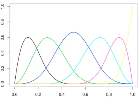
3.3.2 SICA Penalty . . . 62
3.3.3 Monotone Transformation on Response . . . 64
3.3.4 SPOT Algorithm . . . 65
3.4 Theoretical Properties . . . 68
3.5 Numerical Results . . . 71
3.5.1 Effectiveness on Synthetic Data . . . 71
3.5.2 Role of Parameterain Variable Selection . . . 75
3.5.3 Real Data Application . . . 78
3.6 Discussions . . . 81
3.7 Technical Proofs and More Simulation Examples . . . 81
3.7.1 Technical Proofs . . . 82
3.7.2 More Simulation Examples . . . 85
4 Maximum Correlation-based Statistical Dependence Measures . . . 89
4.1 Introduction . . . 89
4.2 Maximum Correlation Coefficient and Optimal Transformation . . . 90
4.3 Dependence Measure . . . 91
4.3.1 Univariate Case: BMC and T-BMC . . . 91
4.3.2 Multivariate Case: MBMC and T-MBMC . . . 98
4.4 Hypothesis Testing . . . 100
4.5 Numerical Results . . . 103
4.5.1 Simulation Results for BMC/T-BMC . . . 103
4.5.2 Simulation Results for MBMC/T-MBMC . . . 104
4.6 Discussions . . . 107
4.6.1 On Dependence Measures . . . 107
4.6.2 On Application to Sufficient Dimension Reduction . . . 108
4.7 Technical Proofs . . . 109 4.7.1 Proof of Theorem 4.3.1 . . . 109 4.7.2 Proof of Theorem 4.3.2 . . . 109 4.7.3 Proof of Theorem 4.3.6 . . . 109 5 Summary . . . 111 VITA. . . 122
LIST OF TABLES
Table Page
2.1 Average MMS and RSD (in parentheses) for Example 2.4.1 . . . 34
2.2 Average MMS and RSD (in parentheses) for Example 2.4.2 . . . 35
2.3 Average MMS and RSD (in parentheses) for Example 2.4.3 . . . 37
2.4 Top ranked (Rank 1 and Rank 2) genes for Example 2.4.4 . . . 38
2.5 AdjustedR2 (in percentage) of fitting 3 different models for Example 2.4.4 . 39 3.1 Comparison of different methods on simulated data from Example 3.5.1. . 73
3.2 Comparison of different methods on simulated data from Example 3.5.2. . 74
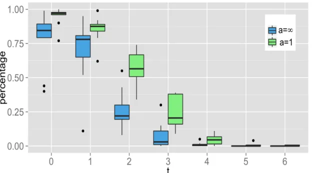
3.3 Average percentages of times that the true model can be selected by SPOT-SICA with different choices of a. The last column corresponds to the result from SPOT-LASSO. . . 77
3.4 Comparison of different methods on simulated data from Example 3.7.1. . 87
LIST OF FIGURES
Figure Page
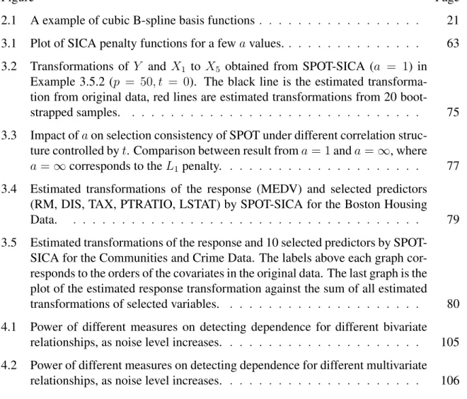
2.1 A example of cubic B-spline basis functions. . . 21
3.1 Plot of SICA penalty functions for a fewavalues. . . 63
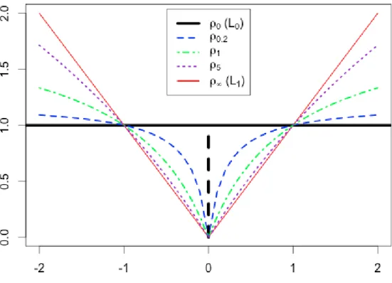
3.2 Transformations of Y and X1 to X5 obtained from SPOT-SICA (a = 1) in
Example 3.5.2 (p = 50, t = 0). The black line is the estimated
transforma-tion from original data, red lines are estimated transformatransforma-tions from 20
boot-strapped samples. . . 75
3.3 Impact ofaon selection consistency of SPOT under different correlation
struc-ture controlled byt. Comparison between result froma= 1anda =1, where
a=1corresponds to theL1 penalty. . . 77
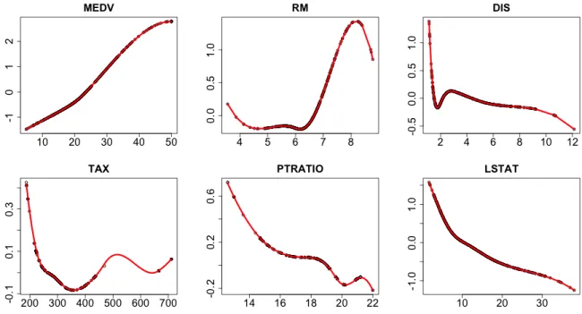
3.4 Estimated transformations of the response (MEDV) and selected predictors (RM, DIS, TAX, PTRATIO, LSTAT) by SPOT-SICA for the Boston Housing
Data. . . 79
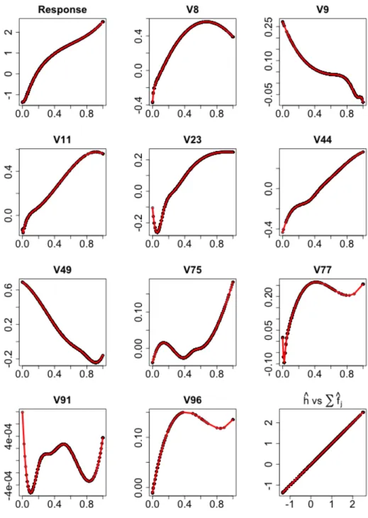
3.5 Estimated transformations of the response and 10 selected predictors by SPOT-SICA for the Communities and Crime Data. The labels above each graph cor-responds to the orders of the covariates in the original data. The last graph is the plot of the estimated response transformation against the sum of all estimated
transformations of selected variables. . . 80
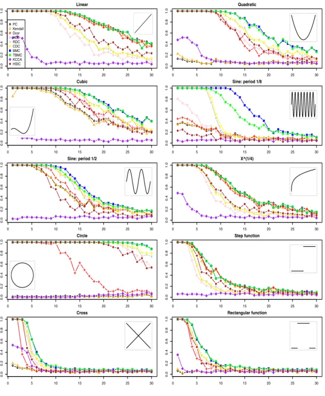
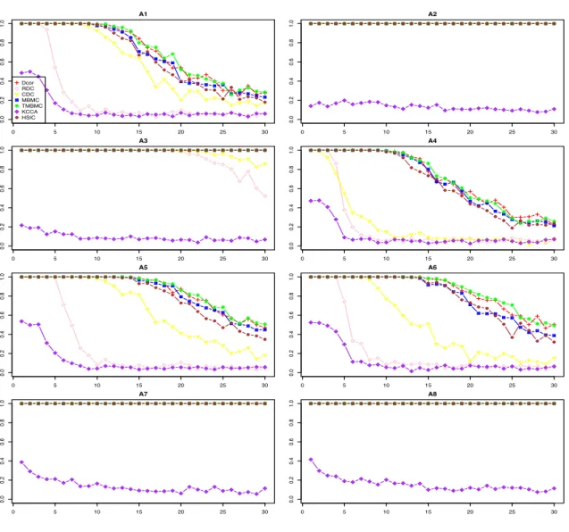
4.1 Power of different measures on detecting dependence for different bivariate
relationships, as noise level increases. . . 105
4.2 Power of different measures on detecting dependence for different multivariate
ABBREVIATIONS
ACE Alternating Conditional Expectation
BMC B-spline-based Maximum Correlation, using the largest eigenvalue
CV Cross Validation
DC-SIS Distance Correlation-based Sure Independence Screening
IQR Inter-Quantile Range
LLA Local Linear Approximation
MBMC Multivariate version of B-spline-based Maximum correlation, using
the largest eigenvalue
MC-SIS Maximum Correlation-based Sure Independence Screening
MMS Mimimal Model Size
MSE Mean Squared Error
NIS Nonparametric Independence Screening
RKHS Reproducing Kernel Hilbert Space
RSD Robust Standard Deviation
SICA Smooth Integration of Counting and Absolute deviation
SIS Sure Indepedence Screening
SPAM SParse Additive Model
SPOT SParse Optimal Transformation
SPOT-LASSO SParse Optimal Transformation withL1penalty
SPOT-SICA SParse Optimal Transformation with SICA penalty
T-BMC B-spline-based Maximum Correlation, using Trace
T-MBMC Multivariate version of B-spline-based Maximum Correlation, using
ABSTRACT
Huang, Qiming PhD, Purdue University, August 2016. Model-Free Variable Screening, Sparse Regression Analysis and Other Applications with Optimal Transformations . Major Professor: Michael Yu Zhu.
Variable screening and variable selection methods play important roles in modeling high dimensional data. Variable screening is the process of filtering out irrelevant vari-ables, with the aim to reduce the dimensionality from ultrahigh to high while retaining all important variables. Variable selection is the process of selecting a subset of relevant vari-ables for use in model construction. The main theme of this thesis is to develop variable screening and variable selection methods for high dimensional data analysis. In particular, we will present two relevant methods for variable screening and selection under a unified framework based on optimal transformations.
In the first part of the thesis, we develop a maximum correlation-based sure indepen-dence screening (MC-SIS) procedure to screen features in an ultrahigh-dimensional set-ting. We show that MC-SIS possesses the sure screen property without imposing model or distributional assumptions on the response and predictor variables. MC-SIS is a model-free method in contrast with some other existing model-based sure independence screening methods in the literature. In the second part of the thesis, we develop a novel method called SParse Optimal Transformations (SPOT) to simultaneously select important variables and explore relationships between the response and predictor variables in high dimensional nonparametric regression analysis. Not only are the optimal transformations identified by SPOT interpretable, they can also be used for response prediction. We further show that SPOT achieves consistency in both variable selection and parameter estimation.
Besides variable screening and selection, we also consider other applications with op-timal transformations. In the third part of the thesis, we propose several dependence mea-sures, for both univariate and multivariate random variables, based on maximum correlation
and B-spline approximation. B-spline based Maximum Correlation (BMC) and Trace BMC (T-BMC) are introduced to measure dependence between two univariate random variables. As extensions to BMC and T-BMC, Multivariate BMC (MBMC) and Trace Multivariate BMC (T-MBMC) are proposed to measure dependence between multivariate random vari-ables. We give convergence rates for both BMC and T-BMC.
Numerical simulations and real data applications are used to demonstrate the perfor-mances of proposed methods. The results show that the proposed methods outperform other existing ones and can serve as effective tools in practice.
1. INTRODUCTION
One common goal for data analysis is to discover the underlying dependence structure
be-tween the response Y and predictor vector X = (X1, X2, . . . , Xp)T, which can be fully
captured by the conditional distribution P(Y|X). Different regression models have been
proposed to characterize the dependence structure, from a limited sample of Y and X.
Regression models differ in several aspects, such as model flexibility, interpretability, com-putational efficiency and prediction accuracy.
Model flexibility and interpretability have been recognized to play key roles in practical data analysis. A general nonparametric regression model,
Y =f(X,✏), (1.1)
or a simplified versionY =f(X) +✏where✏is a random error, is the most flexible model
in regression setting. It assumes no structure constraints on the functionf, and can
accom-modate any possible interactions among those predictor variables. However, this approach suffers severely from the curse of dimensionality, and would generally result in poor esti-mation efficiency. Moreover, the generation process of the response is described much like
a ’black-box’ mechanism by the single joint multivariate function f which consists of all
covariates, making the model hard to be interpretable. A linear model
Y =
p
X
j=0
jXj+✏, (1.2)
on the other extreme, is highly interpretable due to its assumed linear additive structure. Moreover, the additive structure provides a convenient assessment of the individual con-tribution from each predictor variable. However, a reliance on the rigid parametric form limits its ability to model nonlinear effects of the predictor variables.
Different approaches have been proposed to remedy the disadvantages of general non-parametric regression models and linear models, which can achieve a higher degree of
model flexibility than linear models, and obtain better interpretability and computation
ef-ficiency than nonparametric regression models. One approach is to transform responseY
such as Box-Cox transformations, which lead to
T(Y) =
p
X
j=0
jXj+✏. (1.3)
Box and Cox (1964) proposed a family of power transformations on the response forT(Y),
which aims to make the assumptions of linearity, normality and homogeneous variance in linear models more appropriate after transformation. Additive models in Stone (1985),
Y =
p
X
j=1
fj(Xj) +✏, (1.4)
which are different from Box-Cox transformations, allow transformations on each predic-tor variable. Additive models assume that each additive component is a univariate smooth function of a single predictor variable, thus providing nonparametric extensions of linear models and can offer a higher degree of flexibility. And the additive combination of uni-variate functions is more interpretable and easier to fit than general nonparametric models. Despite the popularity of Box-Cox transformations and additive models, their effectiveness are still vulnerable to model mis-specifications, and they could be ineffective for simple
cases like Y = log(X1 +X2
2 +✏). In addition, another drawback of Box-Cox
transfor-mations is that the parametric form of transformation on the response can be restrictive in some applications.
To further improve the model flexibility and interpretability from Box-Cox transforma-tions and additive models, transformation models are proposed, where general
nonparamet-ric transformations are applied to both Y andX. Transformation models are formulated
as h(Y) = p X j=1 fj(Xj) +✏, (1.5)
wherehandfj, j = 1, . . . , p,are arbitrary measurable functions of corresponding random
variables. Under certain conditions, it is shown that transformationshandfj, j = 1, . . . , p,
Chiappori et al., 2015). With the strengths provided by nonlinear transformations and ad-ditive structure, transformation models achieve a good balance in model flexibility and interpretability.
For data analysis, it is an ideal case that the underlying dependence structure between
Y and Xis known so that a precise model can be specified and corresponding model
pa-rameters can be accurately estimated. However, such prior knowledge is seldom given in practice. To explore their relationship, it is a common practice to apply different model structures to approximate the true structure. The choice of a specific model involves dif-ferent considerations over various factors such as model flexibility, interpretability, compu-tational efficiency, prediction accuracy, etc. To combine the advantages of both nonlinear transformation and the additive structure as in (1.5), we consider optimal transformation defined in Breiman and Friedman (1985) and propose several methods in the areas of vari-able screening, varivari-able selection, dependence measure, sufficient dimension reduction, etc.
1.1 Optimal Transformation 1.1.1 Formal Definition
Breiman and Friedman (1985) proposed to apply general nonparametric
transforma-tions to bothY andX and considered optimal transformations by solving a minimization
problem. min h2L2(PY),fj2L2(P Xj) Eh{h(Y) p X j=1 fj(Xj)}2 i , s.t. E[h(Y)] = E[fj(Xj)] = 0; E[h2(Y)] = 1,E[fj2(Xj)]<1. (1.6)
Here,PY andPXj denote the marginal distributions ofY andXj, respectively, and L
2(P)
denotes the class of square integrable functions under the measureP. We denote the
solu-tion to (1.6) ash⇤ andf⇤
transforma-tions forY and X, respectively. Problem (1.6) tries to find transformations that produce the best-fitting additive model. Knowledge of such transformations can aid in the interpre-tation and understanding the relationship between the response and predictors. From the aspect of applying transformation, both Box-Cox transformations and additive models can be considered as special cases of optimal transformations.
A set of sufficient conditions is given in Breiman and Friedman (1985, Section 5.2) for the existence of optimal transformations. Note that under some restrictive conditions, the optimal transformations from (1.6) are equivalent to the transformations in regression model (1.5). However, the equivalence property does not hold in general. The necessary conditions which ensure the equivalence property is still an open research question. Despite this theoretical gap, the optimal transformation approach is still a useful statistical tool in exploring the relationship between the response and predictor variables. In addition, it provides a general framework under which several methods can be proposed.
1.1.2 Applications of Optimal Transformations
Based on optimal transformation, we propose several methods to deal with different statistical problems in next few chapters, including variable screening, sparse nonparamet-ric regression, dependence measure and sufficient dimension reduction. Here, we briefly introduce these methods and show their connections with optimal transformations.
Variable Screening
Variable screening is the process of filtering out irrelevant variables, with the aim to re-duce the dimensionality from ultrahigh to high while retaining all important variables prior to model building. In Chapter 2, we propose a screening procedure based on a dependence measure maximum correlation (R´enyi, 1959), which is defined by
⇢⇤(Y, X) = sup ✓, {
where⇢is the Pearson correlation, and✓and are Borel-measurable functions of univariate
random variablesY andX.
Breiman and Friedman (1985) derived the relationship between the optimal
transfor-mations from (1.6) and maximum correlation. For bivariate cases wherep = 1, the
opti-mal transformations are equivalent to the transformations that yield maximum correlation. Since maximum correlation is a measure that can sensitively capture dependence between the response and the predictor variable in univariate cases, we build a screening procedure which ranks the predictor variables according to their marginal maximum correlations with the response. Maximum correlation is not directly computable because the maximization in (1.7) is taken over infinite-dimensional spaces. Therefore, we approximate the optimal transformations in order to numerically evaluate maximum correlation. The resulting pro-cedures are essentially proposed based on optimal transformations for univariate cases with
p= 1.
Sparse Nonparametric Regression
Optimal transformations only enjoy good statistical and computational behaviors when
the number of variables p is not large to the sample sizen, their usefulness is limited in
the high dimensional setting. In Chapter 3, we extend optimal transformations to deal with high dimensional problems by proposing a sparse version of optimal transformations,
which penalizes the sum ofL2norm of each function componentfj in (1.6). The resulting
optimal transformations encourage parsimonious solutions and perform model selection and parameter estimation simultaneously. To make the optimal transformation interpretable and suitable for regression analysis, we further consider monotone transformation on the
responseY.
Dependence Measures
Due to the fact that maximum correlation between random variables X andY is zero
hypothesis “random variablesXandY are independent”. Beside the maximum correlation
r1and the optimal transformations✓1, 1 defined by
r1 = max
✓1, 12L2(P)
⇢(✓1(Y), 1(X)), (1.8)
one can also define subsequent maximum correlations and optimal transformations. For
functions{✓i, i;i= 1,2, . . .}with bounded positive second moments, let
ri = max ✓i, i2L2(P) ⇢(✓i(Y), i(X)), h✓i(Y),✓j(Y)iL2(PY) = 0, h i(X), j(X)iL2(PX) = 0, (1.9)
for allj = 1, . . . , i 1. Here,h·,·iis the inner product defined in correspondingL2spaces.
Under independence of random variablesXandY, all the values ofri’s are zero. Based
on this property, we propose several independence measures. Since all correlationsri are
not directly computable, we again approximate optimal transformations in order to numer-ically evaluate maximum correlation. Under the framework of optimal transformations, we develop dependence measures by approximating optimal transformations using B-spline basis functions. Given a sample, the optimal transformations are obtained by solving an equivalent eigen problem. Additionally, eigenvalues from the eigen problem correspond to
the values ofri’s. In Chapter 4, we apply the leading eigenvalue, as well as the sum of all
eigenvalues for measuring dependence.
Sufficient Dimension Reduction
The goal of a traditional linear sufficient dimension reduction procedure is to find a few
linear combinations >
1 X, . . . , d>Xthat can fully representX, without loss of information
onY. It is required that those linear combinations satisfy the constraints,
Y ??X|{ >
1 X, . . . , d>X}.
That is, Y is conditionally independent ofX given { >
1 X, . . . , d>X}. Equivalently, the
dependence structure ofY onXis expressed by the regression model
Li (1991) proposed Sliced Inverse Regression (SIR) that can recover the space spanned by 1, . . . , dunder some mild conditions. SIR is connected to a maximization problem as follows. Define
R2(b) = max
T ⇢(T(Y), b
>X) (1.10)
where⇢is the Pearson correlation, T is any squared integrable function, andbis a vector
of length p. We look for the direction b1 which maximizes R2(b), and continue to find
subsequent directionsb2, . . . , bd, satisfying the following conditions.
Cov(b>i X, b>jX) = 0, fori6=j R2(bi) = max
b R
2(b) (1.11)
It is shown in Chen and Li (1998) that the resulting directionsb1, . . . , bdare equivalent
to the directions obtained by SIR. Therefore, solving the maximization problem above can
be viewed as a procedure to recover the space spanned by{ 1, . . . , d}.
One possible way to improve SIR is to generalize dimension reduction from linear to
nonlinear cases, where we consider additive terms of transformed X instead of its linear
combinations. We apply the optimal transformations and extract the transformations ofX
successively, similar to the procedure described in (1.8) and (1.9) of extracting the sequence of maximum correlations. This direction of research is briefly discussed at the end of Chapter 4.
For comparison purposes, we review some existing methods on variable screening and variable selection in high dimension data analysis.
1.2 Review on Variable Screening Methods
In a seminar paper, Fan and Lv (2008) proposed Sure Independence Screening (SIS) for screening variables in linear models. More screening procedures are developed after SIS for other specific models, including screening methods for generalized linear models (Fan and Song, 2010), multi-index models (Zhu et al., 2011) and additive models (Fan et al., 2011), varying coefficient models (Fan et al., 2014), etc. Another kind of screening procedures is developed without imposing any specific model assumption, for example, the
distance correlation-based sure independence screening Li et al. (2012b). In this section, we review three typical screening methods.
1.2.1 Sure Independence Screening (SIS)
Consider a linear regression model
Y =
p
X
j=0
jXj +✏ (1.12)
where✏ is a random error. Fan and Lv (2008) suggested ranking all predictors according
to their marginal Pearson correlations with the response and select the top predictors with
relatively larger Pearson correlation values with a given sample. Letwj =⇢(Y, Xj)where
⇢denotes the Pearson correlation, andwcj be its sample estimates fromnobservations. SIS
retains the following set of predictors.
d
M ={1j p:|cwj|is among the first[ n]largest of all}
where is a pre-defined constant with 2 (0,1), and[ n] denote the integer part of n.
For linear model (1.12), the true set of important predictors is defined as
M? ={1j p: j 6= 0}.
Under some regularity conditions, Fan and Lv (2008) showed that SIS possesses the sure screening property in the ultrahigh dimensional setting, that is,
Pr(M? ✓Md)!1, asn! 1.
1.2.2 Nonparameteric Independence Screening (NIS)
To screening features in ultrahigh dimensional additive model
Y =
p
X
j=0
mj(Xj) +✏ (1.13)
where E{mj(Xj)} = 0. Fan et al. (2011) proposed to rank all predictors according to
E{f2
and{Xij}ni=1, the functionfj(Xj)can be estimated through any basis expansion methods
such as B-splines. Denote its sample estimate as fcnj, NIS retains the following set of
predictors.
d
M⌫ ={1j p:||fcnj||2n ⌫n}
where ||fcnj||2n = n 1
Pn
i=1fcnj(Xij) and⌫n is a pre-specified value. For additive model
(1.13), the true set of important predictors is defined as
M? ={1j p: Em2j(Xj)>0}.
Under some regularity conditions, Fan et al. (2011) showed that NIS possesses the sure screening property for additive models.
1.2.3 Distance Correlation-based Sure Independence Screening (DC-SIS)
Both SIS and NIS are proposed for targeted classes of specified models and may be-come ineffective when the model is mis-specified. To overbe-come this difficulty, Li et al. (2012b) proposed a model-free screening procedure, DC-SIS, to screen features in the ul-trahigh dimensional setting, without imposing any specific model assumptions. DC-SIS uses a dependence measure called distance correlation introduced in Szekely et al. (2007) to
rank the predictor variables. The distance correlation between two random vectoru2Rdu
andv2Rdv is defined by
dcorr(u,v) = p dcov(u,v)
dcov(u,u)dcov(v,v)
wheredcov(·,·)is called distant covariance and defined as follows.
dcov2(u,v) =
Z
Rdu+dv k
u,v(t,s) u(t) v(s)k2w(t,s)dtds
where u(t)and v(s)are the respective characteristic functions of the random vectorsu
andv, u,v(t,s)is the joint characteristic function ofuandv, and
w(u,v) ={cducdv||t|| 1+du du ||s|| 1+dv dv } 1
Distant correlation is a generalization of the Pearson correlation and can be used to cap-ture nonlinear relationships between any two random vectors. Denote the sample estimates
of distant correlation between Y and Xj by dcorr(Y, X[ j), DC-SIS ranks the predictors
according todcorr[2(Y, Xj)and retains the set of predictors
c
M={1j p:dcorr[2(Y, Xj) cn }. Define the true set of important predictors by
M? ={1j p:F(Y|X)functionally depends onXj},
Li et al. (2012b) proved that DC-SIS has the sure screening property under some regularity conditions, without imposing any specific model assumptions.
1.3 Review of Variable Selection Method in Regression
Classical variable selection procedures, which differ from variable screening, perform model selection and parameter estimation simultaneously. The majority of these procedures select variables by minimizing a penalized objective function with the following form.
Loss function+Penalization (1.14)
The most popular choices of loss functions are least squares, negative log-likelihood, and their variants. The penalization part penalizes model complexity and encourages sparsity in the final model. Early methods of variable selection include best subset selection or step-wise (forward/backward) selection with a criterion like Akaike information criterion (AIC)
(Akeike, 1973), Bayesian information criterion (BIC) (Schwarz et al., 1978), Mallow’sCp
(Mallows, 1973), etc. These methods are computational expensive and quickly becomes infeasible as dimensionality grows. Furthermore, the subset selection approaches suffer from instability and their theoretical properties are difficult to examine (Breiman, 1996). In high dimensional data analysis, regularization methods have been proposed to overcome these difficulties. We review some popular methodologies on variable selection in both linear models and additive models.
1.3.1 The Lasso and Its Variants
For linear models (1.2), a standard way of performing variable selection is to penalized least square with a proper choice of the penalty function. One example is the bridge
estima-tor (Frank and Friedman, 1993) which uses the`q-norm (q > 0) of the slope coefficients.
When0 < q 1, some slope estimate can be exactly zero with proper choices of tuning
parameters.
Among all bridge estimators with different choices of q, the most popular estimator is
the one withq= 1, known as the least shrinkage and selection operator (Lasso) proposed in
Tibshirani (1996). The Lasso estimates of the coefficients are the solution to the following optimization problem. min 1,..., p E 2 4 Y p X j=0 jXj !23 5 subject to p X j=1 | j|L; (1.15)
which is also equivalent to the standard form as in (1.14),
min 1,..., p E 2 4 Y p X j=0 jXj !23 5+ p X j=1 | j|; (1.16)
whereLand are tuning parameters.
Least Angle Regression (LARS) algorithm (Efron et al., 2004) gives the entire solution path of the Lasso estimate. In addition, Lasso estimates can also be computed efficiently via coordinate descent algorithms (Fu, 1998; Friedman et al., 2007). It is shown that Lasso can consistently select the true model under the Irrepresentable Condition (Zhao and Yu, 2006).
Other variants of Lasso includes the grouped lasso (Yuan and Lin, 2006), the elastic net (Zou and Hastie, 2005), the fussed lasso (Tibshirani et al., 2005), the adaptive lasso (Zou,
2006), etc. Beside the`1 penalty, other penalty functions are investigated in the literature,
1.3.2 Variable Selection in Additive Models
There are several approaches to generalize variable selection from linear to non-linear models, in particular, the additive models (1.4). One typical example is the Sparse Additive Model (SPAM) proposed in Ravikumar et al. (2007). They consider a modification of standard additive model optimization problem as follows.
min gj2HXj E 2 4 Y p X j=1 jgj(Xj) !23 5 s.t. p X j=1 | j|L,E[gj2(Xj)] = 1; (1.17)
whereLis a pre-defined constant.
Denote = ( 1, . . . , p)>. Then, the constraint that lies in the`1ball{ :|| ||1 1}
encourages sparsity of the estimated , just as for the Lasso (Tibshirani, 1996).
Let fj = jgj, we can re-express the minimization problem (1.17) in the following
equivalent Lagrangian form:
1 2E 2 4 Y p X j=1 jfj(Xj) !23 5+ p X j=1 q E[f2 j(Xj)] (1.18)
where is the regularization parameter.
Ravikumar et al. (2007) developed a backfitting algorithm, named SPAM, to estimate
the functions fj (j = 1, . . . , p) for a given sample. They further showed that SPAM can
consistently select all important functional components under some regularity conditions. Other approaches of variable selection in additive models include Meier et al. (2009), Huang et al. (2010) and Balakrishnan et al. (2012), where different penalty functions are used to produce sparse estimates of the functional components.
1.4 Outline
In this thesis, we study and propose several new methodologies for variable screening, sparse nonparametric regression, dependence measures and dimension reduction, under
the unified framework with optimal transformations. In Chapter 2, we develop a maximum correlation-based sure independence screening (MC-SIS) procedure to screen features in an ultrahigh-dimensional setting. In Chapter 3, we develop a novel method called SParse Optimal Transformations (SPOT) to simultaneously select important variables and explore relationships between the response and predictor variables in high dimensional nonpara-metric regression analysis. In Chapter 4, we propose several dependence measures based on maximum correlation and B-spline approximation, and discuss the application of opti-mal transformations in nonlinear sufficient dimension reduction. Chapter 5 summaries the results of this thesis.
2. MODEL-FREE SURE SCREENING VIA MAXIMUM
CORRELATION
2.1 Introduction
With the rapid development of modern technology, various types of high-dimensional data are collected in a variety of areas such as next-generation sequencing and biomedical imaging data in bioinformatics, high-frequency time series data in quantitative finance, and spatial-temporal data in environmental studies. In those types of high-dimensional data,
the number of variablespcan be much larger than the sample sizen, which is referred to as
the ‘largepsmalln’ scenario. To deal with this scenario, a commonly adopted approach is
to impose the sparsity assumption that the number of important variables is small relative
to p. Based on the sparsity assumption, a variety of regularization procedures have been
proposed for high-dimensional regression analysis such as the lasso (Tibshirani, 1996), the smoothly clipped absolute deviation method (Fan and Li, 2001), and the elastic net
(Zou and Hastie, 2005). All these methods work when p is moderate. However, when
applied to analyze ultrahigh-dimensional data where dimensionality grows exponentially
with sample size (e.g., p = exp(n↵) with ↵ > 0), their performances will deteriorate
in terms of computational expediency, statistical accuracy and algorithmic stability (Fan et al., 2009). To address the challenges of ultrahigh dimensionality, a number of marginal screening procedures have been proposed under different model assumptions. They all share the same goal that is to reduce dimensionality from ultrahigh to high while retaining all truly important variables. When a screening procedure achieves this goal, it is said to have the sure screening property in the literature.
Fan and Lv (2008) proposed to use the Pearson correlation for feature screening and showed that the resulting procedure possesses the sure screening property under the lin-ear model assumption. They refer to the procedure as the Sure Independence Screening
(SIS) procedure. Fan and Song (2010) extended SIS from linear models to generalized linear models by using maximum marginal likelihood values. Fan et al. (2011) developed a Nonparametric Independence Screening (NIS) procedure and proved that NIS has the sure screening property under the additive model. Li et al. (2012b) proposed to use dis-tance correlation to rank the predictor variables, and showed that the resulting procedure, denoted as DC-SIS, has the sure screening property without imposing any specific model assumptions. Compared with the other screening procedures discussed previously, DC-SIS is thus model-free. Distance correlation was introduced in Szekely et al. (2007), which uses joint and marginal characteristic functions to measure the dependence between two random variables. We briefly review the SIS, NIS, DC-SIS procedures here.
From the review above, it is clear that the standard approach to developing a valid screening procedure consists of two steps. First, a proper dependence measure between the response and predictor variables needs to be defined and further used to rank-order all the predictor variables; and second, the sure screening property needs to be established for the screening procedure based on the dependence measure. The screening methods discussed previously differ from each other in these two steps. For example, SIS uses the Pearson correlation as the dependence measure and possesses the sure screening property under linear models, whereas NIS uses the goodness of fit measure of the nonparametric regression between the response and predictor variable as the dependence measure and possesses the sure screening property under additive models.
For the purpose of screening in an ultrahigh dimensional setting, we argue that an ef-fective screening procedure should employ a sensitive dependence measure and satisfy the sure screening requirement without model specifications. The goal of screening is not to precisely select the true predictors, instead, it is to reduce the number of predictor vari-ables from ultrahigh to high while retaining the true predictor varivari-ables. Therefore, false positives or selections can be tolerated to a large degree, and sensitive dependence mea-sures are more preferred than insensitive meamea-sures. In ultrahigh dimensional data, there usually does not exist information about the relationship between the response and predic-tor variables, and it is extremely difficult to explore the possible relationship due to the
presence of a large number of predictors. Therefore, model assumptions should be avoided as much as possible in ultrahigh dimensional screening, and we should prefer screening procedures that possess the sure screening property without model specifications. In other words, model-free sure screening procedures are more preferable. Among the existing screening procedures discussed previously, only DC-SIS is model-free because it does not require any restrictive model assumption. However, the distance correlation measure used by DC-SIS may not be sensitive especially when the sample size is small, because empirical characteristic functions are employed to estimate distance correlations.
A more sensitive dependence measure between the response and a predictor variable is the maximum correlation, which was originally proposed by Gebelein (1941) and studied by R´enyi (1959) as a general dependence measure between two random variables. R´enyi (1959) listed seven fundamental properties that a reasonable dependence measure must have, and maximum correlation is one of a few measures that can satisfy this requirement. The definition and estimation of maximum correlation involve maximizations over func-tions (see Section 2.2.1), and thus it is fairly sensitive even when the sample size is small. Recently, there have been some revived interests in using maximum correlation as a proper dependence measure in high-dimensional data analysis (Bickel and Xu, 2009; Hall and Miller, 2011; Reshef et al., 2011; Speed, 2011).
We propose to use maximum correlation as a dependence measure for ultrahigh dimen-sional screening, and prove that the resulting procedure has the sure screening property without imposing model specifications (see Theorem 2.2.2 in Section 2.2.4). We adopt the B-spline functions-based estimation method from Burman (1991) to estimate maximum correlation. We refer to our proposed procedure as the Maximum Correlation-based Sure Independence Screening procedure, or in short, the MC-SIS procedure. Numerical results show that MC-SIS is competitive to other existing model-based screening procedures, and is more sensitive and robust than DC-SIS when the sample size is small or the distributions of the predictor variables have heavy tails.
The rest of this chapter is organized as follows. In Section 2.2, we introduce maximum correlation and the B-spline functions-based method for estimating maximum correlation,
propose the MC-SIS procedure, and establish the sure screening property for MC-SIS. In Section 2.3, we develop a three-step procedure for selecting tuning parameters for MC-SIS in practice. Section 2.4 presents results from simulation studies and a real life screening application. Section 2.5 provides additional remarks on the screening methods and future research directions. The proofs of the theorems are given in Section 2.6.
2.2 Independence Screening via Maximum Correlation
In this section, we formally introduce the proposed screening procedure MC-SIS, which uses maximum correlation as the dependence measure. We first introduce its connection to optimal transformation in Section 2.2.1, and then propose to use B-spline function to approximate optimal transformation in Section 2.2.2, which leads to a proper approximated evaluation of maximum correlation. Based on the approximation, we propose MC-SIS in Section 2.2.3. Sure screening property of MC-SIS is established in Section 2.2.4.
2.2.1 Maximum correlation and optimal transformation
Recall that Y is the response variable and X = (X1, . . . , Xp) the vector of predictor
variables. We assume the supports of Y andXj (j = 1, . . . , p)are compact, and they are
further assumed to be [0,1] without loss of generality. For any given j, consider a pair
of random variables (Xj, Y). The maximum correlation coefficient between Xj and Y,
denoted as⇢⇤
j, is defined as follows.
⇢⇤j(Xj, Y) = sup
✓, {
⇢(✓(Y), (Xj)) : 0<E{✓2(Y)}<1,0<E{ 2(Xj)}<1}, (2.1)
where⇢ is the Pearson correlation, and✓ and are Borel-measurable functions of Y and
Xj. We further denote ✓j⇤ and ⇤j as the optimal transformations that attain the maximum
correlation.
Maximum correlation coefficient enjoys the following properties given in R´enyi (1959):
(a) 0⇢⇤
j(Xj, Y)1;
(b) ⇢⇤
(c) ⇢⇤
j(Xj, Y) = 1if there exist Borel-measurable functions✓⇤and ⇤such that✓⇤(Y) =
⇤(X
j);
(d) ifXj andY are jointly Gaussian, then⇢⇤j(Xj, Y) =|⇢(Xj, Y)|.
Some other properties of maximum correlation coefficient are discussed in Szekely and Mori (1985), Dembo et al. (2001), Bryc and Dembo (2005), and Yu (2008). Due to Property (d), it is clear that maximum correlation is a natural extension of the Pearson correlation. Note that the Pearson correlation does not possess Properties (b) and (c). For Property (c),
there are cases that the Pearson correlation coefficient can be as low as zero when Y is
functionally determined byXj. For example, ifY =X12 whereX1 ⇠N(0,1), the Pearson
correlation betweenY andX1is zero, whereas the maximum correlation is one. Therefore,
maximum correlation is a more proper measure of the dependence between two random variables than the Pearson correlation.
R´enyi (1959) established the existence of maximum correlation under certain sufficient conditions, and a different set of sufficient conditions are given in Breiman and Friedman
(1985). Breiman and Friedman (1985) also showed that optimal transformations✓⇤
j and ⇤j
can be obtained via the following minimization problem. min ✓j, j2L2(P) e2 j = E[{✓j(Y) j(Xj)}2], subject to E{✓j(Y)}= E{ j(Xj)}= 0; E{✓j2(Y)}= 1. (2.2)
Here,Pdenotes the joint distribution of (Xj,Y) andL2(P)is the class of square integrable
functions under the measure P. Let e⇤2
j be the minimum of e2j. Breiman and Friedman
(1985) derived two critical connections between e⇤2
j , squared maximum correlation ⇢⇤j2,
and optimal transformation ⇤
j, which we state asFact 0below.
Fact 0. e⇤j2 = 1 ⇢⇤j2; (2.3a)
Fact 0 suggests that the minimization problem (2.2) is equivalent to the optimization problem (2.1). Furthermore, the squared maximum correlation coefficient is equal to the
expectation of the squared optimal transformation ⇤
j.
Various algorithms have been proposed in the literature to compute maximum corre-lation, including Alternating Conditional Expectations (ACE) in (Breiman and Friedman, 1985), B-spline approximation in Burman (1991), and polynomial approximation in Bickel and Xu (2009) and Hall and Miller (2011). Equation (2.3b) indicates that maximum
cor-relation coefficient ⇢⇤j can be calculated through the optimal transformation ⇤j. In this
chapter, we apply Burman’s approach to first estimate ⇤
j, and then estimate⇢⇤j, which will
be further used in screening.
2.2.2 B-spline estimation of optimal transformations
LetSn be the space of polynomial splines of degree` 1and{Bjm, m = 1, . . . , dn}
denote a normalized B-spline basis with||Bjm||sup 1, where||·||sup is the sup-norm. We
have ✓nj(Y) = ↵>jBj(Y), nj(Xj) = j>Bj(Xj) for any✓nj(Y), nj(Xj) 2 Sn, where
Bj(·) = (Bj1(·), . . . , Bjdn(·))> denotes the vector ofdnbasis functions. Additionally, we
letkbe the number of knots wherek =dn `. One example of the B-spline basis functions
is depicted in Figure 2.1.
The population version of B-spline approximation to the minimization problem (2.2) can be written as follows.
min ✓nj, nj2Sn E[{✓nj(Y) nj(Xj)}2], subject to E{✓nj(Y)}= E{ nj(Xj)}= 0; E{✓2nj(Y)}= 1. (2.4)
Burman (1991) applied a technique to remove the first constraintE{✓nj(Y)}= E{ nj(Xj)}=
0in the optimization problem above as follows. First, letz1, . . . ,zdn 1(zi = (zi1, . . . , zidn)>
fori= 1, . . . , dn 1) bedn-dimensional vectors which are orthogonal to each other,
orthog-onal to the vector of 1’s andzT
izi = 1fori= 1, . . . , dn 1. Second, obtain matrixDj with the(s, m)-entryDj,sm = zsm/(kbjm)where bjm = E{Bjm(Xj)}, for s = 1, . . . , dn 1
Figure 2.1. A example of cubic B-spline basis functions
and m = 1, . . . , dn. Third, let nj(Xj) = ⌘j> j(Xj) where j(Xj) = DjBj(Xj).
With this construction, it is easy to verify that E{ nj(Xj)} = 0, and the minimization
ofE[{✓nj(Y) nj(Xj)}2]subject toE{✓nj2 (Y)} = 1 ensures thatE{✓nj(Y)} = 0.
Bur-man (1991) showed the equivalence between the optimization problem (2.4) and the one stated below. min ✓nj, nj2Sn E[{✓nj(Y) nj(Xj)}2], subject to E{✓nj2 (Y)}= 1. (2.5)
For fixed✓nj(Y)(i.e., fixed↵j), the minimizer of (2.5) with respect to⌘j and nj(Xj)
are
⌘j = [E{ j(Xj) j>(Xj)}] 1E{ j(Xj)B>j(Y)}↵j,
nj(Xj) = >j (Xj)[E{ j(Xj) j>(Xj)}] 1E{ j(Xj)B>j (Y)}↵j.
(2.6)
max
↵j2Rdn
↵>jE{Bj(Y) j>(Xj)}[E{ j(Xj) j>(Xj)}] 1E{ j(Xj)B>j (Y)}↵j,
subject to ↵>jE{Bj(Y)B>j (Y)}↵j = 1.
(2.7) Following the notation in Burman (1991), we denote
Aj00 = E{Bj(Y)B>j (Y)}, AjXX = E{ j(Xj) j>(Xj)},
AjX0 = E{ j(Xj)B>j (Y)}, and Aj0X =A>jX0.
It is clear that (2.7) is a generalized eigenvalue problem, which can be solved by the
largest eigenvalue and its corresponding eigenvector ofAj001/2Aj0XAjXX1 AjX0Aj001/2. We
denote the largest eigenvalue by ⇤
j1, which is equal to ||A
1/2
j00 Aj0XAjXX1 AjX0Aj001/2||,
where || · || is the operator norm, and further denote the corresponding eigenvector by
↵⇤j. Let ⇤nj(Xj) = >j (Xj)[E{ j(Xj) j>(Xj)}] 1E{ j(Xj)Bj>(Y)}↵⇤j. ⇤nj can be
considered the spline approximation to the optimal transformation ⇤
j defined previously.
Note that the target function in (2.7) isE( ⇤2
nj), and we also haveE( ⇤nj2) = ⇤j1.
Given the data {Yu}nu=1 and{Xuj}nu=1, we estimate Aj00, AjXX, AjX0, andAj0X as
follows. d Aj00 =n 1 n X u=1 Bj(Yu)B>j(Yu), A\jXX =n 1 n X u=1 bj(Xuj)b>j (Xuj), [ AjX0 =n 1 n X u=1 bj(Xuj)B>j (Yu), and A[j0X =A[jX0 > ,
where bj(Xuj) = DcjBj(Xuj), the (s, m)-entry ofDcj isDbj,sm = zsm/(kbcjm), andbcjm =
n 1Pn
u=1Bjm(Xuj), fors = 1, . . . , dn 1andm= 1, . . . , dn. Then, ⇤j1 is estimated by
c⇤ j1 =||Adj00 1/2 [ Aj0XA\jXX 1 [ Aj0X > d Aj00 1/2 ||, and ↵⇤
j is estimated by the eigenvector of Adj00
1/2 [ Aj0XA\jXX 1 [ Aj0X > d Aj00 1/2 corre-sponding to c⇤
j1, which we denote as ↵c⇤j. Therefore, the optimal transformation of Y is
estimated by✓c⇤
nj =↵c⇤j
>
Bj(Y). Furthermore, based on (2.6), the optimal transformation of
Xj can be obtained by c⇤nj =⌘cj⇤ > j(Xj)with⌘cj⇤ =A\jXX 1 [ AjX0↵c⇤j.
Based on the two relationships (i)E( ⇤2
j ) = (⇢⇤j)2 and (ii)E( ⇤nj2) = ⇤j1, and the fact
that ⇤
njis the optimal spline approximation to ⇤j, we propose to screen important variables
using the magnitudes of c⇤
2.2.3 MC-SIS procedure
Let ⌫n be a pre-specified threshold, andDd⌫n the collection of selected important
vari-ables. Then, our proposed screening procedure can be defined as
d
D⌫n ={1j p: c⇤j1 ⌫n}. (2.8)
Empirically, the threshold value⌫n is often set so that|Dd⌫n|=nor[n/lnn]as in Fan and
Lv (2008) and Fan et al. (2011), where|Dd⌫n|is the cardinality ofDd⌫n and[a]denotes the
integer part ofa. Since c⇤
j1is the estimate of ⇤j1, which is an approximation to the squared
maximum correlation coefficient⇢⇤2
j , we refer to the procedure as the MC-SIS procedure.
2.2.4 Sure Screening Property
We establish the sure screening property of the MC-SIS procedure in this section. The
sure screening property is a property under the asymptotic regime that the sample size n
goes to infinity and the number of predictor variables (denoted as pn) may grow with n.
The regime with a fixed number of predictor variables, which ispn =pfor alln >0, can
be considered a special case. We first introduce some notations.
For any givenn, following Li et al. (2012b), we useFn(Y|X)to denote the conditional
distribution of Y given X. Note that the subscript n in Fn is used to indicate that the
conditional distribution of Y givenX can depend onnbecause bothY andXdepend on
pnandpnmay grow withn. DefineAn ={j :Fn(y|X)functionally depends onXj}and
En ={j : ⇢⇤j(Y, Xj) > 0}. Let Acn ={j : Fn(y|X)does not functionally depend onXj}
andEc
n ={j : ⇢⇤j(Y, Xj) = 0}. Note that bothAnandEn can change withn asngoes to infinity.
The predictor variables in An are the true predictors that jointly affect the response
variableY. The predictor variables inEnare those that have positive maximum correlations
with Y. In some cases, An is a subset of En, whereas in some other cases, An is not a
subset of En. It is known that a predictor variable can be a true predictor variable, but it
procedures in the literature, our proposed MC-SIS procedure will fail to retain the true
predictor variable. DefineDn = An \En, andDnc = Acn[Enc. We refer to the predictor
variables in Dn as the active predictor variables, and those in Dnc the inactive predictor
variables.
The goal of the MC-SIS procedure is to retain the active predictor variables. Recall
thatDd⌫n is the collection of predictor variables selected by MC-SIS. The probability that
d
D⌫n contains Dn, which is Pr(Dn ✓ Dd⌫n), is not expected to be one when based on a
finite sample. Instead, we aim to identify reasonable sufficient conditions under which the
probabilityPr(Dn ✓Dd⌫n)converges to one asngoes to infinity. This property is referred
to as the sure screening property in the literature.
We first consider the special case in which the active setDnis fixed. Under this special
case, there exists a positive constant c, such that minj2Dn⇢j⇤(Y, Xj) > c > 0 for any n,
indicating that the marginal maximum correlation coefficients between the response and
active predictor variables are always bounded away from zero by the constant c. For this
special case, we can show that as the sample size n goes to infinity and some additional
conditions hold, the probability that MC-SIS can retain Dn converges to one; In other
words, MC-SIS possesses the sure screening property.
We next consider the general case in which the active set Dn can change and diverge
as n increases. For each n, define cn = minj2Dn⇢⇤j(Y, Xj). Clearly, cn is the smallest
maximum correlation coefficient between the response and the active predictor variables for
givenn. Under the assumption that there exists a constantc > 0such that asymptotically
cn is bounded away from zero by the constant c, that is, lim infn!1cn > c, the sure
screening property of MC-SIS can be established. Although this assumption is broader than the special case discussed previously, it is still too restrictive.
When the sample size increases, we should allow the possibility that cnmay decrease
to zero. The rate at whichcndecreases to zero plays a critical role in determining whether
MC-SIS possesses the sure screening property. If the rate is too fast, the correlation between the response and some active predictor variables becomes too weak, and MC-SIS may fail to retain those active predictor variables, and thus MC-SIS fails to possess the sure
screening property. On the other hand,dn, which is the number of B-spline basis functions used in MC-SIS, critically affects the performance of MC-SIS. The success of MC-SIS
hinges on the interplay of dn and cn as n goes to infinity. In this article, we impose a
mild condition on this interplay between cn and dn, which controls the relative rates of
cn and dn as n goes to infinity. This condition is listed as Condition 5 or (C5) below.
Under (C5) and other regularity conditions, we show that MC-SIS indeed possesses the sure screening property (see Theorem 2.2.2). Note that the two special cases discussed above automatically satisfy (C5); Therefore, Theorem 2.2.2 implies that MC-SIS is a sure screening procedure for these two special cases.
Before stating the theorems regarding the theoretical properties of MC-SIS, we first list the conditions below.
(C1) If the transformations✓j and j with zero means and finite variances satisfy
✓j(Y) + j(Xj) = 0a.s., then each of them is zero a.s.
(C2) The conditional expectation operators E{ j(Xj) | Y} : H2(Xj) ! H2(Y)and
E{✓j(Y) | Xj} : H2(Y) ! H2(Xj) are all compact operators. H2(Y) and H2(Xj) are
Hilbert spaces of all measurable functions with zero mean, finite variance and usual inner product.
(C3) The optimal transformations{✓⇤
j, ⇤j}
p
j=1 belong to a class of functionsF, whose
rth derivativef(r)exists and is Lipschitz of order↵
1, that is,F ={f :|f(r)(s) f(r)(t)|
K|s t|↵1 for alls, t}for some positive constantK, wherer is a nonnegative integer and
↵1 2(0,1]such thatd=r+↵1 >0.5.
(C4) The joint density ofY andXj (j = 1, . . . , p)is bounded and the marginal
(C5) The number of B-spline basis functionsdnsatisfies thatdn min
j2Dn
(⇢⇤2
j )/(2c1n 2),
for some constantc1 >0and constantwhere0< d/(2d+ 1).
(C6) There exist positive constant C1 and constant ⇠ 2 (0,1) such that dnd 1
c1(1 ⇠)n 2/C1.
Conditions (C1) and (C2) are adopted from (Breiman and Friedman, 1985), which en-sure that the optimal transformations exist. Conditions (C3) and (C4) are from Burman (1991), but modified for our two-variable scenario. Condition (C5) above is similar to Condition 3 in Fan and Lv (2008), Condition C in Fan et al. (2011), and Condition (C2) in Li et al. (2012b), which all require that the dependence between the response and active predictor variables cannot be too weak. As discussed earlier in this section, this condition is necessary since a marginal screening procedure will fail when the marginal dependence between the response and an active predictor variable is too weak.
The following lemma shows that the maximum correlations achieved by B-spline-based transformations are at the same level as the original maximum correlations.
Lemma 2.2.1 Under conditions (C3) – (C6), we have min
j2Dn
⇤
j1 c1⇠dnn 2.
Based on condition (C1) – (C6), we establish the following sure screening property for MC-SIS.
Theorem 2.2.2 (a) Under conditions (C1) – (C4), for any c2 > 0, there exist positive
constantsc3andc4 such that Pr( max
1jp|c ⇤
j1 ⇤j1| c2dnn 2)O(p⇣(dn, n)). (2.9)
(b) Additionally, if conditions (C5) and (C6) hold, by taking ⌫n = c5dnn withc5
c1⇠/2, we have that
Pr(Dn✓Dd⌫n) 1 O(s⇣(dn, n)), (2.10)
wheresis the cardinality ofDn.
Note that Theorem 2.2.2 is stated in terms of a fixed number of predictor variables p.
In fact, the same theorem holds for a divergent number of predictor variables, which is
denoted aspn. As long aspn⇣(dn, n)goes to zero asymptotically, MC-SIS can possess the
sure screening property. We remark that the number of basis functionsdnaffects the final
performance of MC-SIS. To obtain the sure screening property, an upper bound of dn is
o(n1/7). Since d
n is determined by the choices of the degree of B-spline basis functions
and the number of knots, different combinations of degree and the number of knots can lead to different screening results. Additionally, knots placement can further affect the behavior of B-spline functions, and in practice, knots are usually equally spaced or placed at sample quantiles. In next section, we will propose a data-driven three-step procedure for
determiningdnfor MC-SIS in practice. The optimal choice ofdnand knots placement are
beyond the scope of this thesis and can be an interesting topic for future research.
The sure screening property from Theorem 2.2.2 guarantees that MC-SIS retains the active set. The size of the selected set can be much larger than the size of the active set. Therefore, it is of interest to assess the size of the selected set. Following an approach in Fan et al. (2011), we establish such a result for MC-SIS and state it in the next theorem.
Theorem 2.2.3 Under Conditions (C1) – (C6), we have that for any⌫n = c5dnn , there
exist positive constantsc3 andc4such that Pr{|Dd⌫n|O n
2 max(⌃)
} 1 O(pn⇣(dn, n)), (2.11)
where|Dd⌫n|is the cardinality ofDd⌫n, max(⌃)is the largest eigenvalue of⌃,⌃= E( >), = ( >
1, . . . , p>n)
>, p
defined in Theorem 2.2.2.
From Theorem 2.2.3, we have that when max(⌃) = O(n⌧), the cardinality of the
selected set by MC-SIS will be of order O(n2+⌧). Thus, by applying MC-SIS, we can
reduce dimensionality from the original exponential order to a polynomial order, while retaining the entire active set.
2.3 Tuning Parameter Selection
In the previous section, we show that in order to achieve the sure screening property
of MC-SIS, we need to impose several conditions on the choice of dn. Recall dn = k+
`, where k is the number of knots and ` is the degree of the B-spline basis functions.
These conditions are of theoretical interest, but cannot be directly implemented in practice. It is well known that the performance of B-spline functions in nonparametric regression
depends on the choices ofk and`as well as the placement of knots. This is also the case
for the performance of MC-SIS under a given finite sample.
Several rules of thumb have been proposed to choose dn for B-spline basis functions
when used for the purpose of screening in the literature. For example, cubic splines with
dn =
⇥
n1/5⇤ + 2 were used in Fan et al. (2011), and cubic splines with d
n =
⇥
2n1/5⇤
were proposed in Fan et al. (2014), and in both works, the knots were placed at the sample quantiles. These rules of thumb can also be applied to MC-SIS, however, we found their performances are not so satisfactory in some models we have experimented with. In this
section, we propose a more effective approach for selecting`andk (ordn) of the B-spline
basis functions for MC-SIS.
There are two major factors in the use of B-spline basis functions, which affect the performance of MC-SIS. The first factor is the complexity of the B-spline basis functions
characterized by ` and k. The larger ` and k are, the more complex the B-spline basis
functions. Using more complex basis functions can clearly lead to the overfitting problem for inactive predictor variables, many of which may be retained due to their falsely inflated
empirical correlations with the response variable. On the other hand, using less complex
basis functions with small`andkcan lead to the underfitting problem for active predictor
variables, that is, the maximum correlations between the response variable and active pre-dictor variables may be underestimated, and some active prepre-dictor variables may be ranked
lower due to underestimated maximum correlations. Therefore, the proper selection of `
andk hinges on the balance between the overfitting and underfitting problems.
The other factor that affects the performance of MC-SIS is whether the same choices
of`andkare used for all predictor variables, which is referred to as theunified scheme, or
different choices of`andkare used for different predictor variables, which is referred to as
theseparate scheme. The unified scheme treats all predictor variables the same way and is relatively simple, but it may be appropriate for some variables while being inappropriate for other variables. It is difficult to find a unified scheme that simultaneously fits all predictor variables. On the other hand, the separate scheme allows individual variables to choose their most suitable basis functions, but it has two drawbacks. The first drawback is that it may exacerbate the overfitting problem for inactive predictor variables, and the second is that its computational demand is high.
Based on the discussion above, it is clear that for the purpose of screening, an ideal scheme for choosing basis functions for MC-SIS is to use the unified scheme with simple basis functions for inactive predictor variables and the separate scheme with complex basis functions for active predictor variables. This ideal scheme is not feasible in practice because we do not know which predictor variables are active and which are inactive ahead of time. In what follows next, we instead propose a data-driven three-step approach to approximate the ideal scheme. Because B-spline basis functions of degree higher than three are seldom
used in practice, we only consider ` 2 {1,2,3}. Furthermore, we always place knots at
sample quantiles.
In the first step, we use the unified scheme with B-spline basis functions of degree
one. In other words, we fix` = 1. The number of knots k is then determined as follows.
Consider a set of candidate values for k, for example, K1 k K2, where K1 and
between the response variable and the predictor variables using k knots and ` = 1, and
then we fit a two-component Gaussian mixture distribution to the calculated maximum
correlations and denote the resulting component means as µ1(k) andµ2(k), respectively.
The Gaussian mixture distribution is used to cluster predictor variables into two groups with one group including large maximum correlations and the other including small ones. Letd(k) =|µ1(k) µ2(k)|, which is a measure of separability of those two groups. The
largerd(k)is, the more separable the two groups are. We want to choose the value ofkthat
can separate the two groups the most. A natural choice isk˜ = minK
1kK2d(k). Then,
we apply MC-SIS with ` = 1and k = ˜k to all of the predictor variables, and retain B1
predictor variables with the largestB1 maximum correlations, whereB1 is a pre-specified
number. The purpose of using the unified scheme with linear B-spline basis functions in this step is to avoid the overfitting problem and screen out a large number of inactive predictor variables.
In the second step, we employ the separate scheme. For each remaining predictor
variable, an M-fold Cross-Validation (CV) procedure is used to select ` 2 {1,2} and k
(where K1 k K2), where M is a pre-defined integer. The maximum correlation
between the predictor variable and the response variable is then calculated using B-spline
basis functions with the selected`andk. Subsequently, we rank-order the predictors using
their corresponding maximum correlations and retain the topB2predictor variables, where
B2 is a pre-specified number. TheM-fold CV procedure uses the correlation between the
response variable and the predictor variable as the score function. The purpose of using the separate scheme and B-spline basis functions of higher degree is to correct the under-fitting problem possibly suffered by the active predictor variables in the first step.
The third step is similar to the second step. The only difference is that the degree `
for B-spline basis functions is selected from {1,2,3} instead of {1,2}. In other words,
for individual remaining predictor variables, B-spline basis functions of degree up to three may be used to calculate their maximum correlations. The purpose of using cubic spline basis functions is to provide sufficient capacity to calculate the maximum correlations of active predictor variables.
The maximum correlations for all pairs of(Y, Xj)are calculated based on their selected
tuning parameters. The predictor variables are then sorted, and the topB3 are retained as
the final output of MC-SIS, whereB3is a pre-specified number.
Note that the three-step procedure proposed above requires three pre-specified
num-bers,B1,B2 andB3. The choices ofB1, B2 andB3can vary from one problem to another
and depend on a number of factors, including the sample size n, the number of predictor
variables p, the signal strengths of the active variables, the noise level, etc. How to
opti-mally determineB1,B2andB3is beyond the scope of this thesis. Here, we instead provide
some general guidelines for the user in practice. Suppose the user has a conservative lower
bound, denoted asq1, for the number of predictor variables that are independent of the
re-sponse, and a conservative upper bound, denoted asq2, for the number of active variables.
For example, suppose there are 500 predictor variables in an application problem. Apply-ing the sparsity principle, the user believes that a half of the predictors are independent of
the response variable. Then,q1 can be assumed to be 200. Furthermore, the user believes
that the number of true variables is less than 20. Then,q2 can be set as 20.
The goal of the first step in the three-step procedure is to screen out inactive predictor
variables which are independent of the response, andB1 is the number of predictor
vari-ables that can enter the second step. A proper choice ofB1 isB1 =p q1. In the previous
example,B1then becomes 300, and is conservative in that the first step eliminates 200 out
of all 250 predictors that are independent of the response. Similarly, B2 is the number of
predictor variables that can enter the third step so that the maximum correlations of active predictor variables can be accurately evaluated. In order to not leave out any active
vari-ables from the third step, a proper choice ofB2isB2 =q2. Again in the previous example,
B2 is set to be 20. BecauseB3is the number of predictor variables that are retained in the
output setDd⌫n defined in Section 2.2.3, the choice ofB3 is equivalent to the choice of⌫n.