An SSVEP Brain-Computer Interface: A Machine Learning Approach

University of Mississippi University of Mississippi

eGrove

eGrove

Electronic Theses and Dissertations Graduate School

1-1-2012

An SSVEP Brain-Computer Interface: A Machine Learning

An SSVEP Brain-Computer Interface: A Machine Learning

Approach

Approach

Fei Teng

University of Mississippi

Follow this and additional works at: https://egrove.olemiss.edu/etd

Part of the Computer Sciences Commons

Recommended Citation Recommended Citation

Teng, Fei, "An SSVEP Brain-Computer Interface: A Machine Learning Approach" (2012). Electronic Theses and Dissertations. 1374.

AN SSVEP BRAIN-COMPUTER INTERFACE: A MACHINE LEARNING APPROACH

A Dissertation

submitted in partial fulfillment of requirements for the degree of Ph.D

in the Department of Computer and Information Science The University of Mississippi

by FEI TENG

Copyright Fei Teng 2012 ALL RIGHTS RESERVED

ABSTRACT

A Brain-Computer Interface (BCI) provides a bidirectional communication path for a human to control an external device using brain signals. Among neurophysiological features in BCI systems, steady state visually evoked po-tentials (SSVEP), natural responses to visual stimulation at specific frequen-cies, has increasingly drawn attentions because of its high temporal resolution and minimal user training, which are two important parameters in evaluat-ing a BCI system. The performance of a BCI can be improved by a properly selected neurophysiological signal, or by the introduction of machine learning techniques. With the help of machine learning methods, a BCI system can adapt to the user automatically.

In this work, a machine learning approach is introduced to the design of an SSVEP based BCI. The following open problems have been explored:

1. Finding a waveform with high success rate of eliciting SSVEP.

SSVEP belongs to the evoked potentials, which require stimulations. By comparing square wave, triangle wave and sine wave light signals and their corresponding SSVEP, it was observed that square waves with 50%

duty cycle have a significantly higher success rate of eliciting SSVEPs than either sine or triangle stimuli.

2. The resolution of dual stimuli that elicits consistent SSVEP.

Previous studies show that the frequency bandwidth of an SSVEP stim-ulus is limited. Hence it affects the performance of the whole system. A dual-stimulus, the overlay of two distinctive single frequency stimuli, can potentially expand the number of valid SSVEP stimuli. However, the improvement depends on the resolution of the dual stimuli. Our ex-perimental results showed that 4 Hz is the minimum difference between two frequencies in a dual-stimulus that elicits consistent SSVEP.

3. Stimuli and color-space decomposition.

It is known in the literature that although low-frequency stimuli (<

30Hz) elicit strong SSVEP, they may cause dizziness. In this work, we explored the design of a visually friendly stimulus from the perspective of color-space decomposition. In particular, a stimulus was designed with a fixed luminance component and variations in the other two dimen-sions in the HSL (Hue, Saturation, Luminance) color-space. Our results showed that the change of color alone evokes SSVEP, and the embedded frequencies in stimuli affect the harmonics. Also, subjects claimed that a fixed luminance eases the feeling of dizziness caused by low frequency

flashing objects.

4. A machine learning approach.

Machine learning techniques have been applied to make a BCI adaptive to individuals. An SSVEP-based BCI brings new requirements to ma-chine learning. Because of the non-stationarity of the brain signal, a clas-sifier should adapt to the time-varying statistical characters of a single user’s brain wave in realtime. In this work, the potential function clas-sifier is proposed to address this requirement, and achieves 38.2bits/min on offline EEG data.

ACKNOWLEDGEMENTS

Thanks Dr. Yixin Chen for teaching me how to be a researcher. Thanks Dr. Scott Gustafson and Dr. Dwight Waddell for providing all the supports. Thanks Dr. Paul Ruth for helping me make the bluetooth work. Thanks Dr. Pamela Lawhead, Aik Min Choong and Chirstopher Reichley for great advises and helps on the design of the amplifier.

TABLE OF CONTENTS

ABSTRACT i

ACKNOWLEDGEMENTS iv

LIST OF FIGURES viii

LIST OF TABLES xiv

1 INTRODUCTION 1

1.1 Introduction . . . 1

1.2 A Brain-Computer Interface . . . 2

1.3 The Bit Rate of a BCI . . . 6

1.4 Outline of this Dissertation . . . 7

2 BACKGROUND 12 2.1 Feature Extraction . . . 12

2.1.1 P300 . . . 14

2.1.2 Motor Imagery . . . 15

2.1.3 SSVEP . . . 17

3 AN EFFECTIVE STIMULUS 23

3.1 Methodology . . . 23

3.2 Results and Conclusions . . . 27

4 DUAL AND TRI-STIMULI 32 4.1 Methodology . . . 32

4.2 Results and Conclusions . . . 34

5 STIMULI AND COLOR-SPACE DECOMPOSITION 37 5.1 Methodology . . . 37

5.2 Results and Conclusions . . . 41

6 POTENTIAL FUNCTION CLASSIFIER 44 6.1 Introduction . . . 45

6.2 Background . . . 46

6.3 Potential Function Rules . . . 53

6.4 Potential Function Rules and The Bayes Decision Theory . . . 54

6.5 Potential Function Rules as Plug-in Decision Rules . . . 61

6.5.1 An Approximation on Multi-class Potential Function classifiers 62 6.5.2 The Potential Gap and the Generalization Performance . . . 65

6.6 A Generalization Bound for Potential Function Classifiers . . . . 69

6.8 Experimental Results of the Model Selection Method . . . 85

6.8.1 Synthetic Data . . . 85

6.8.2 Comparison with Leave-one-out Classifier Selection . . . 90

6.8.3 Conclusions . . . 91

6.9 Experimental Results over SSVEP Data . . . 93

7 FUTURE WORK 96

BIBLIOGRAPHY 99

LIST OF FIGURES

Figure Number Page

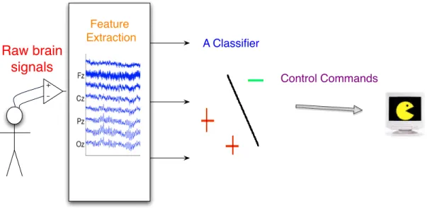
1.1 A BCI translates brain signals into commands. It collects raw brain activity, processes it into features, and then uses a

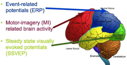
clas-sifier to decode these features. . . 3 1.2 A brief schematic of the brain by Young (146). The primary visual

cortex is at the back of the brain in the occipital lobe. The primary motor cortex is located in the posterior portion of the frontal lobe. The strongest P300 signal is typically measured

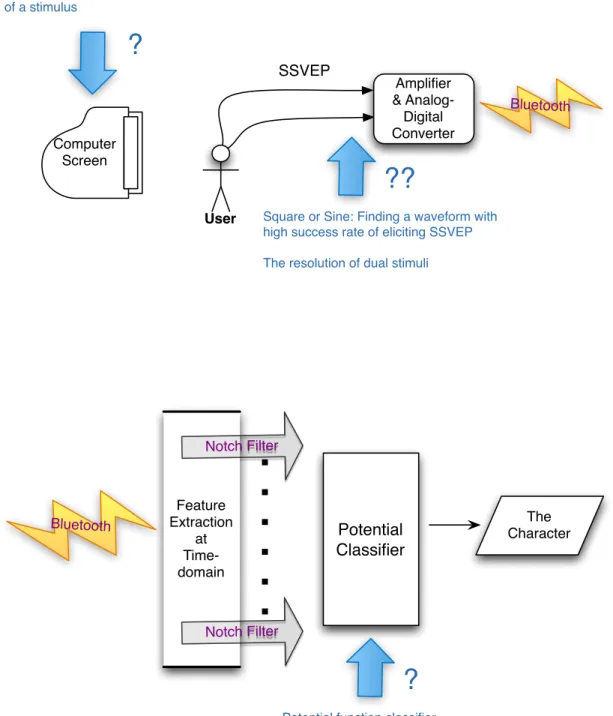
at the parietal lobe. . . 5 1.3 Open problems investigated in this work are marked by question

marks with arrows pointing to where they occur. A computer screen generates visual stimuli. The Amplifier collects the EEG signal and uses Bluetooth to send it to software-notch-filters and a potential function classifier, which outputs the

2.1 A P300 interface from the Brain-Computer Interface Laboratory at East Tennessee State University. This P300 system high-lights the characters randomly, and waits for the P300 peak that appears in the user’s brain after she notices the wanted

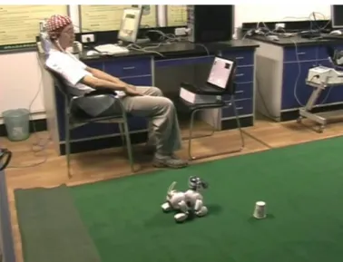
character being highlighted. . . 15 2.2 A motor-imagery system from the Tsinghua University. This

sys-tem detects the activation in the user’s motor cortex when the user simulates a given action in his brain, and translates this

activity into commands to control the robot dog on the floor. . 16 2.3 An SSVEP system at the University of Bremen. The user focuses

on light sources blinking with different frequencies (the light-emitting diodes at the bottom of the screen). The frequency that is currently in the focus lets the neurons in the visual cortex of the brain synchronize with the same frequency. By detecting the frequency at which the user is looking, the system

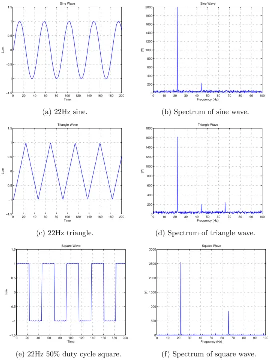
3.1 (a), (c), and (e) are the luminance figures of a LED measured by a Lutron LX-102 light meter. Their corresponding frequency representations are given in (b), (d), and (f), respectively. The spectrum of the square wave strictly adheres to theory, that is, a peak demonstrated at fundamental frequency f as well as a peak at the 3f harmonic. The sine wave and the triangle wave do not. They have weak harmonics that should not exist at 2f. However, these harmonics should not affect the result since

their strength are one tenth that of the fundamental frequency. 25 3.2 11, 13, 15, 18 and 22Hz were used as the stimulus frequencies.

The accuracies of the SSVEP experiments are computed with

equation Accuracy = _{T otal trials}1f occurs . . . 29 4.1 Spectrums of SSVEP for dual stimuli. . . 34 4.2 Spectrums of SSVEP for tri stimuli. . . 35

5.1 In the HSL color-space, the luminance is fixed, while the hue and the saturation vary along a trajectory. Frequencies are delivered by the change of the Hue and Saturation together (the closed curve), by the change of the Hue only (the H axis, figure(c)(d)) or by the change of Saturation only (the S axis, figure(e)(f)). A cycle begins at a certain point on the curve and ends when the trajectory of the stimulus hits this point again. The changes in the SL space can be continuous

or discrete. . . 40

5.2 Spectrums of SSVEP of three types of stimulation. The stimulus

is a 12Hz flashing square on a computer screen. . . 42 6.1 Considering a straight line is used as the classifier to separate the

”+” points from the ”-” points. It is intuitive that any three points that do not fall on a same straight line can be shattered by this model (left), while some set of four points can not be shattered (right). Thus, the VC dimension of this particular

6.2 Sample class potential functions and margins under a 3-class sce-nario. (a) The solid curve describes the variation of margin

γ(x,3,S) with respect to the sample class potential φ3(x,S)

when the sample class potentialφ1(x,S) andφ2(x,S) are fixed.

The dashed curve represents ξ, the bounded amount by which the margin is less than α = 0.3. (b) The three curves rep-resent sample class potential functions built upon 12 training observations (denoted by the markers on the horizontal axis) using a 1-d sinc point potential function with s = 0.1. Each arrow corresponds to a margin, which is computed as the dif-ference between the vertical coordinate of the tip of the arrow and that of the end of the arrow. The numeric value of the margin is given along with the arrow. The arrow is absent if

the margin is 0. . . 70 6.3 (a) Plots of ξi, the bounded margin shortage, as a function of the

margin γ(xi, zi,S(i)). When α approaches 0, ξ_αi converges to the indicator function I(xi, zi,S(i)). (b) Plots of the upper bound on the probability of error in (6.19) as a function of the

6.4 Distributions of margin and normalized margin under a Gaussian point potential function e−kx−yk

2

σ2 with different values of σ. . . 83

6.5 Comparing the sample potential function classifier with the Bayes classifier on a synthetic data set. (a) Joint probability density functions for each category. (b) A point-wise comparison of the probability thatfS is different fromf∗ with the normalized potential gap. (c) The posterior gap of the synthetic data. (d) The difference between the posterior gap and the normalized

LIST OF TABLES

Table Number Page

3.1 Statistics of harmonics in SSVEP . . . 28

4.1 SSVEP at different combinations of stimulus frequencies. . . 36

5.1 HSL Space Stimuli HSL and RGB Values in One Cycle . . . 39

5.2 Statistic of harmonics in SSVEP . . . 42

6.1 The comparison results of model selection using leave-one-out er-ror and the margin distribution metric defined in (6.28). . . . 92

6.2 Statistic of PFRs over Offline SSVEP Data . . . 94

6.3 Statistic of PFRs over Offline SSVEP Data 2 . . . 94

Chapter 1

INTRODUCTION

1.1

Introduction

A brain-computer interface translates brain activities into commands that control external devices. The BCI research began in the early 1970s. At that time Jacques Vidal built a first BCI based on visual evoked potentials (134; 135).

This research field was initially motivated by the need for a new type of communication tools for paralyzed or elderly people, whose brains work per-fectly but whose muscles do not (60; 18; 143). While they have lost all other communication abilities, the brain might be the last opportunity for them to communicate with the outside world. In recent years, researchers have investigated BCI for healthy people for computer gaming or entertainment applications (100; 72; 62; 101). However, the ability of existing BCIs is very limited and needs to be improved for healthy users (86).

To explain this, the structure of a typical BCI system is described in Sec-tion 1.2, and a general performance measure to evaluate BCIs is introduced

in Section 1.3. In Section 1.4, we outline the open problems that have been explored to make progress toward a better SSVEP-based BCI.

1.2

A Brain-Computer Interface

A typical BCI system is shown in Figure 1.1. It has a measurement unit to collect the brain signal, a signal processing unit to extract features from the neurological activity and a classification unit to decode “thoughts” into control commands.

There are several measurement techniques in BCI systems. These tech-niques can be grouped into invasive methods, which place electrodes within the brain, and non-invasive methods, which place electrodes above the skull. Considering that a healthy person usually do not want to implant electrodes into her head, together with the fact that the EEG is technically easier and less expensive to realize (94), the non-invasive Electroencephalography (EEG) is preferred in many BCI designs.

EEG is a very weak electrical signal that needs to be amplified before it can be processed by a software. At the moment we started our BCI study, the commercial EEG collection device in the lab does not provide access to the raw data. Thus we made an EEG recording device.

Our design can be divided into the analog part and the digital part. The analog part amplifies the EEG signal, and is mainly based on “The OpenEEG

-+ Raw brain signals Feature Extraction _{A Classifier} Control Commands

Figure 1.1: A BCI translates brain signals into commands. It collects raw brain activity, processes it into features, and then uses a classifier to decode these features.

Project”, an open source project helping people build their own EEG devices for free (as in General Public License) (96). In our design, the digital part uses an ATMEGA8L microprocessor to digitize the amplified signals and control a bluetooth module to send data wirelessly to a computer.

Many neurophysiological features can be detected with EEG. It is beyond the scope of this study to supply a complete review of them. Instead, we present a brief review of three most widely used signals, namely SSVEP, motor -imagery and event related potentials.

• Event-related potentials (ERP)

ERP refers to a positive deflection (P300 peak) appears after the user notices a rare or surprising event (19; 143; 101; 127). An ERP-based

BCI is described in Section 2.1.1.

• Motor-imagery (MI) related brain activity

The activation in the user’s motor cortex would increase if she simulates a given action in her brain without actual performance (76; 79). See Section 2.1.2 for an MI-based BCI.

• Steady state visually evoked potentials (SSVEP)

SSVEP refers to signals that are natural responses to visual stimulation at specific frequencies. The user’s EEG would contain periodic wave-forms of the same frequency as the stimulus (84; 67; 68; 92; 34; 47; 125; 89; 126).

A major difference among these features is that the magnitude of the response varies across the brain, as different brain areas are responsible for different tasks. SSVEP, MI and ERP are usually detected at the visual cortex, the primary motor cortex and the parietal lobe, respectively. These locations are illustrated in Figure 1.2.

Other important differences among these features include the temporal resolution (response time) and user training time. Compared with the P300, whose response time is limited by the rareness of the event to evoke ERP, an SSVEP system detects SSVEP peaks that appears in the subject’s brain after around 400ms (108). Compared with the motor-imagery, which requires the

Figure 1.2: A brief schematic of the brain by Young (146). The primary visual cortex is at the back of the brain in the occipital lobe. The primary motor cortex is located in the posterior portion of the frontal lobe. The strongest P300 signal is typically measured at the parietal lobe.

user to be trained beforehand (103), a user’s SSVEP is naturally entrained to the frequency of a given light stimulus (108). Only minimal user training is needed to use an SSVEP-based BCI (95). Consequently, among these choices, SSVEP is viewed as a promising electrophysiological source for BCI systems (16). However, SSVEP does not outperform everything. Same as the P300, low-frequency flashing objects (with a frequency lower than 30 Hz) used by SSVEP BCI as stimuli may cause dizziness or even safety hazards linked to photo-induced epileptic seizures (46; 98; 51).

Finally, features extracted by the signal processing component are decoded by the classifier into control commands. Without the help of machine learning techniques, BCIs will have to use predetermined parameters, which require

users to adjust themselves to the decision rules (134). A machine learning technique can adapt the system to a user through an initial training session. In addition, a realtime adaptation can be implemented to accommodate the non-stationary property of the EEG signal over time.

1.3

The Bit Rate of a BCI

Bit rate is a general performance measure to evaluate BCIs. Let us con-sider two BCI systems, BCI1 and BCI2. Assume that BCI1 can choose one

option out of 20 possible selections with an accuracy of 90%. BCI2 can make

a binary decision with an accuracy of 95%. If these two BCIs are used to pick a symbol from a set of 20 objects, BCI1 will finish the task with one successful

trial while BCI2 will need to make five consecutive correct decisions.

There-fore, BCI1’s success rate is still 90% while BCI2’s drops to 77.4%(= 95%5).

This fact suggests that the bit rate of BCIs needs to take into consideration the accuracy, the number of possible selections and the number of decisions per minute. Thus, the bit rate R of a BCI is computed as the product of the number of bits per decision (B) and the average number of decisions per minute (142). The number of bits per decision B is given by

B = log₂N +P log₂P + (1−P) log₂ 1−P

where N is the number of possible selections, and P is the accuracy.

1.4

Outline of this Dissertation

The goal of this work is to find a better stimulus and a machine learning approach, which introduce adaptiveness, accuracy and speed to an SSVEP BCI. Open problems that have been explored are illustrated in Figure 1.3. From the perspective of the stimulator, research was conducted on finding an effective stimulus (in Section 3), finding the resolution of dual stimuli (in Section 4) and what help color-space decomposition can provide to the design of a visually friendly stimulus (in Section 5). For the classification unit, the Potential Function Classifier (in Section 6) is designed to process the neurological features and adjust to the changes in realtime. These research topics are briefly described below.

• Finding a waveform with high success rate of eliciting SSVEP.

Because the EEG is always mixed with background noises, the efficacy of an SSVEP-based BCI system relies heavily on the signal-noise ra-tio. Intuitively, SSVEP will be detected much easier and faster if the signal-noise ratio is high. The faster an SSVEP is identified, the more promptly a BCI system can respond correctly, hence a higher informa-tion throughput (1). Square wave (with different duty cycles), triangle wave, and sine wave were compared in Section 3 for their success rate of

User Amplifier & Analog-Digital Converter Bluetooth Bluetooth Feature Extraction at Time-domain Notch Filter Notch Filter Potential Classifier Computer Screen SSVEP

Square or Sine: Finding a waveform with high success rate of eliciting SSVEP The resolution of dual stimuli

??

?

HSL color-space decomposition of a stimulus

Potential function classifier

?

The Character

Figure 1.3: Open problems investigated in this work are marked by question marks with arrows pointing to where they occur. A computer screen generates visual stimuli. The Amplifier collects the EEG signal and uses Bluetooth to send it to software-notch-filters and a potential function classifier, which outputs the character that the user wants to input.

eliciting SSVEP. It was observed that the choice of a square wave, tri-angle wave or sine wave light signal visual stimulus affects the strength of the elicited SSVEP. Square wave is with the highest success rate of eliciting SSVEP. Also, researchers observed that a stimulus at frequency

f can elicit SSVEP not only at f, but also harmonics at 2f, 3f, or sometimes even at higher orders (17; 71). This seems to suggest that harmonics may be used in detecting the stimulating frequency. How-ever, in order to take advantage of the harmonics in the design a BCI system, the following question needs to be addressed. Are the harmon-ics in SSVEP elicited by the fundamental frequency, i.e., f, or by the artifacts of the stimulus? It was observed that square waves with 50% duty cycle have a significantly higher success rate than either sine or triangle stimuli, and the success rate of getting harmonics is positively correlated with the strength of the artifacts in a stimulus.

• The resolution of dual stimuli that provides consistent SSVEP.

It was reported that SSVEPs could be elicited in the range of 4–100Hz (106; 59; 50), while the strongest response was observed in the range of 5– 20Hz (34; 47; 68). This fact limits the number of valid stimuli, hence affects the performance of an SSVEP-based BCI. In order to provide more stimuli options within 5−20Hz, dual stimuli were proposed in the

literature. For example, Cheng et al. (35) used multiple color stimuli to deliver two frequencies simultaneously. However, no research has been done on the resolution of the dual stimuli, i.e., what is the resolution of dual stimuli that provides consistent SSVEP? We use dual stimuli, generated by two sine waves on a light emitting diode (LED) to study the resolution needed for consistent responses (Section 4). Our experi-mental results showed that 4 Hz is the minimum difference between two frequencies.

• Stimuli and color-space decomposition.

It is known that low-frequency stimuli (< 30 Hz) tend to elicit strong SSVEP but may cause safety hazards linked to photo-induced epileptic seizures (46; 47). Arakawa et al. (6) showed that both luminance and color patterns elicit SSVEP. However, in their experiments, the lumi-nance was not completely isolated from the color. In this study, we ex-plored a stimulus in the HSL (Hue, Saturation, Luminance) color-space. Stimuli were designed with a fixed luminance component and variations in the other two dimensions in the HSL space. We demonstrate this type of stimulator elicits SSVEP at the fundamental frequency, and the embedded frequencies affect harmonics. Furthermore, all subjects in our experiment felt that this color-space decomposition makes low-frequency

stimuli more visually friendly than ordinary luminance stimuli. • A machine learning approach.

Machine learning techniques adapt the BCI to a subject. Considering the dynamic nature of EEG signals of one user, i.e., the structure of the data may vary over time, the classifier needs to adapt to the changes in realtime. In order to address this problem, we propose the Potential Function Classifier in Chapter 6.3. This algorithm has been tested with datasets from the UCI Machine Learning Repository and offline EEG datas.

Chapter 2

BACKGROUND

BCI is an interdisciplinary research area. Without understanding some important facts from neurophysiology, one cannot see the options and chal-lenges in this field.

This chapter introduces neurophysiological background knowledges. In a BCI, the raw brain signals are processed by feature extraction methods, which are introduced in Section 2.1. Among brain signals, the P300, MI and SSVEP are reviewed with example applications in Section 2.1.1, Section 2.1.2 and Section 2.1.3, respectively. Methods to deliver accurate stimuli using a computer screen are shown in Section 2.1.3. Finally, machine learning techniques that have been deployed in BCIs are discussed in Section 2.1.4.

2.1

Feature Extraction

In most current BCI systems, features used were motivated from neuro-physiological observations. For example, SSVEP BCIs are based on the fact that the users EEG would contain periodic waveforms of the same frequency as the stimulus, thus they use frequencies as their features (88; 90). Also

because of the mechanism P300 and MI occur, BCIs based on them take P300 peak at the parietal, or MI peak lobe at the primary motor cortex, as features.

In applications where the frequency range of interest is given a priori, Fast Fourier Transform (FFT) is widely applied to extract discriminative features in the frequency domain (85; 77; 102; 111). Wavelets transform is another technique that combines spatial and frequency information (45). In time to frequency domain transforms, a high resolution in the frequency-domain can only be achieved using a long time window, i.e., a long data sequence in time-domain. FFT needs x seconds to achieve a _x1Hz resolution, for example, one second of data to achieve one Hz resolution. Considering that the SSVEP appears about 400ms after the stimulation (108), and SSVEP BCIs usually use 1Hz as the difference between stimuli, time-domain features were explored, to extract SSVEP peaks without waiting for a full second (for 1Hz resolution in FFT). For instance, Li et al. (78) used bandpass filters to extract independent features. Kalman filter was used by Neuper’s team (93) and Gage’s team (48).

Many feature extraction methods have been proposed to increase the sig-nal to noise ratio. Among them, Independent Component Asig-nalysis (ICA) receives wide attention (120; 65). ICA is commonly used when multiple EEG

reading are available. It interprets each channel of the recorded EEG data as a linear combination of n unknown but independent sources, then reconstructs the signals. Principal components analysis (PCA) is another technique that was used in (45; 48). It decomposes the EEG data into mutually orthogonal channels. In some applications, signal to noise ratio can be improved by a differential feature extraction approach. For example, common spatial pat-terns (CSP) are computed in motor-imagery systems (78; 43) to identify the source of neurophysiological events.

2.1.1 P300

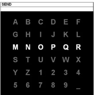
P300 is popularly used for building BCI spellers (19). P300 peak is a positive deflection appears after the user notices a rare or surprising event. For example, a strong P300 peak is detectable near the parietal lobe when letter A is noticed by a user waiting for A but has been shown letter B for some seconds. Figure 2.1 shows a P300 interface used in the Brain-Computer Interface Laboratory at East Tennessee State University. A substantial but unsolvable problem of a P300 is that it is slow to make a P300 peak appear, thus affects the performance of BCIs based on them. This is because the event driving a P300 peak has to be rare enough, e.g., something shown once a second is not rare. Researchers usually improve P300 performance by using a relatively large number of possible selections (36 in (117; 42; 64)).

Figure 2.1: A P300 interface from the Brain-Computer Interface Laboratory at East Ten-nessee State University. This P300 system highlights the characters randomly, and waits for the P300 peak that appears in the user’s brain after she notices the wanted character being highlighted.

In literature, both online and offline P300 BCIs were explored. For exam-ple, online systems were developed in (104) and (141) with bit rates (calcu-lated by Eq.(1.1)) of 9.48 bits/min and 10.88 bits/min, respectively. Offline systems reported in (42) achieved 20.1 bits/min, in (8) 2.65 bits/min, in (37) 5.64 bits/min and 23.75 bits/min in (117). Kaper et al. (64) showed the most promising result of 84.7 bits/min, as a special case on a single subject.

2.1.2 Motor Imagery

The activation in the user’s motor cortex would increase if she simulates a given action in her brain without actual performance. This activity is called the motor-related brain activity. For example. if a user imagines to

Figure 2.2: A motor-imagery system from the Tsinghua University. This system detects the activation in the user’s motor cortex when the user simulates a given action in his brain, and translates this activity into commands to control the robot dog on the floor.

raise her left arm, the activation in her motor cortex will increase. Even better, this increase is distinguishable from imagining raising her right arm. Figure 2.2 shows the motor-imagery related brain activity system used in the Tsinghua University. An problem of MI BCI is that it is not intuitive and takes time (days or even weeks) to learn to imagine movement, thus to use the system (143).

Conversely to the P300, motor imagery systems can make a decision fast (22) but lack of possible selections (2 in (22; 136), 3 in (23; 25), 4 in (24)). In different applications, Blankertz et al. achieved bit rates of 23 bits/min, 6-15 bits/min, 6-15-35 bits/min and 12-35 bits/min in (21), (22), (23), and (25), respectively. A 4.3 bits/min was reported in an online system (136).

Impres-sive MI-based BCIs were shown in “The BCI Competition III”, in which the top three teams achieved 47.4 bits/min, 40.4 bits/min and 37.8 bits/min (24).

2.1.3 SSVEP

SSVEP refers to signals that are natural responses to visual stimulation at specific frequencies. The user’s EEG would contain periodic waveforms of the same frequency as the stimulus (125; 89; 126). Compared to other neurophysiological features in EEG, SSVEP holds the advantage of short/no training time - a user’s SSVEP is naturally entrained to the frequency of a given light stimulus.

Figure 2.3 shows an SSVEP system in the Institute of Automation, Uni-versity of Bremen.

At present, no general conclusion on SSVEP stimuli can be drawn because many conditions have not been tested and variables interact with each other. In literature, the type of stimulation, the frequency, the luminance, the color, the embedded frequencies and the subject’s attention have been considered as attributes affecting SSVEP.

• Stimulation Type

Several types of SSVEP visual stimulators have been introduced and used for years (36; 106; 94; 47), based on the fact that both luminance and color patterns elicit SSVEP, while the power of the SSVEP response

Figure 2.3: An SSVEP system at the University of Bremen. The user focuses on light sources blinking with different frequencies (the light-emitting diodes at the bottom of the screen). The frequency that is currently in the focus lets the neurons in the visual cortex of the brain synchronize with the same frequency. By detecting the frequency at which the user is looking, the system lets him control the robot arm.

is affected by them (107; 6). In 1989, Regan claimed that the SSVEP re-sponse for light stimuli was larger than that for pattern reversal in (106). Wu confirmed this statement by showing that SSVEP response elicited by an LED was larger than that by a rectangle stimulus on a computer screen. This explains why the bit rates of BCIs using LED stimuli are usually higher than those of BCIs using computer screens (29; 137). However, from the viewpoint of implementation, a computer screen is preferred as this type of stimulation mainly relies on software devel-opment and no hardware modification is necessary. Furthermore, re-searchers can set any attributes to any possible value of the stimuli on

screens, no matter the luminance, contrast, color, saturation et al., com-pared to LEDs, over which no accurate control could be achieved1. It is also noteworthy that the PC hardware and operating system may affect the accuracy of the stimulation frequency on a screen (62). Sugiarto and Sutoyo claimed that DirectX, OpenGL and Matlab are effective in implementing an accurate stimulus with a computer screen (123; 124). • The Frequency

The stimulus frequencies used in SSVEP research are usually categorized into three bands: low (1-12Hz), medium (12-30Hz) and high (30-60Hz). SSVEP is strongest in the visual cortex, when the stimulus is flashing at around 15Hz (98).

• The Luminance

Arakawa et al. showed that both luminance and color elicit SSVEP (6). However, in those experiments, the luminance was not completely iso-lated from the color.

• The Color

In1966, Regan found out that red, yellow, and blue light stimuli, to-gether with the chosen frequency, affect SSVEP responses (107). In 2001, Cheng’s group first considered the color of the stimulus as a source

of frequency instead of on/off lights (35). After them, many researcher explored the use of different colors, in which red, white and green are frequently used. Two BCI labs demonstrated that the best-performing color is green (49; 97). But no comparison has been done to show how color influences the SSVEP performance. In Section 5, we completely isolated luminance and color to check if color patterns elicit SSVEP. • The Embedded Frequencies

It is known that SSVEP has the same fundamental frequency as the vi-sual stimulus. If two frequencies were delivered simultaneously, SSVEP would have both (89). Many methods have been used to embed frequen-cies in a single stimulus, for example, different colors (35), or the lumi-nance in LEDs (126). In Section 3, we conclude that frequencies other than the fundamental frequency in a square wave may elicit SSVEP. In Section 4, we conclude that two embedded frequencies in an LED have to be at least 4Hz apart to elicit consistent SSVEP.

• Attention on the stimuli

It has been proved that the SSVEP strength is strongly influenced by at-tention (91). If a subject moves her atat-tention to something else than the flashing stimulus, no matter proactive or passive, the power of SSVEP will decrease. Most researchers solve this problem by moving the flashing

objects along with the controlled elements (81; 132). Specifically, if two stimuli were presented, the SSVEP of the ignored one would decrease and the SSVEP of the selected one would be enhanced (112). Sometimes it is not favorable as we want to take the advantage of multiple stimuli. This problem could be solved by using a single flashing object to deliver multiple frequencies (126).

Despite dizziness or even safety hazards linked to photo-induced epileptic seizures caused by low-frequency flashing objects (with a frequency lower than 30 Hz) (46; 51), SSVEP-based BCIs achieve promising information transfer rates, with flexible number of possible selections, which may vary from 4 in (97), 11 in (137; 34) to 30 in (29). Interestingly, the four-class SSVEP achieved an impressive 51.5 bits/min (an average over 11 subjects), compar-ing with 11-class SSVEPs’ 42 bits/min (137) and 27.15 bits/min (34), or a 17.4 bits/min with 30 classes (29). Promising results were also reported in (138) as 29-63 bits/min and in (63) as 66.7 bits/min.

2.1.4 Machine Learning Techniques in BCIs

Several groups applied machine learning techniques to BCI to adapt the system to users. For example, quadratic discriminant analysis (QDA) was implemented in (93; 115). It achieves the optimality if the data is Gaussian distributed. Linear discriminant analysis (LDA) is used in (93; 115; 43; 70).

It is similar to QDA with a stronger assumption that each class has a same covariance. Regression techniques are applied in (77; 144; 83; 48; 120) to find an optimum function mapping the data to their class labels. Fatourechi (45) and Kirby (70) tested the k-nearest-neighbors (KNN) classifier, which as-signs an unknown data point to the majority class of its k-nearest neighbors. In (111), support vector machines (SVM) were used. SVM separates data with hyperplanes by maximizing the margin. There are also works using neural network classifies (4).

Chapter 3

AN EFFECTIVE STIMULUS

As shown in Figure 1.3, this study works toward a good SSVEP BCI system. Obviously, it needs an effective stimulus to evoke distinguishable SSVEP peaks for further processing. In this chapter, we find an effective stimulus, defined as a stimulus with high success rate of eliciting SSVEP.

3.1

Methodology

A stimulus is a object flashing at a certain frequency, while the frequency could be delivered as a sine wave, or a square wave. If different stimuli per-form differently at evoking SSVEP, among square wave, triangle wave and sine wave light signals, which one has the highest success rate of eliciting SSVEP? Furthermore, from a signal perspective, the commonly used flick-ering stimulus is a periodic square wave with 50% duty cycle. Its spectrum contains nonzero Fourier components at±(2k−1)f,k = 1,2,· · ·. Researchers observed that a stimulus flickering at frequency f can elicit SSVEP not only at frequencyf, but also the harmonics at 2f, 3f, or sometimes even at higher orders (17; 71). Therefore, under a square wave stimulus, the cause of a 3f

harmonic in SSVEP is unclear, i.e., Are the harmonics in SSVEP elicited by the fundamental frequency, i.e., f, or by the artifacts of the stimulus? We explore the SSVEP responses of three periodic stimuli, square waves with different duty cycles, triangle wave, and a sine wave, to answer the above two questions.

Three types of periodic stimulus were used in the experiments: square wave (with duty cycle τ ∈ (0,1)), triangle wave, and sine wave. If we define the relative strength of the k-th harmonic frequency with respect to the fundamental frequency as r(k) = Gk G1

where G1 and Gk are the Fourier

coefficients for the fundamental frequency and the k-th harmonic frequency, respectively, it is straightforward to show that rsine(k) = 1 for k = ±1 and 0

otherwise; rtriangle(k) = _π 2sinc kπ 2 2 ; rsquare(k) = sinc(kτ) sinc(τ) . Clearly, in theory

there are no harmonic frequencies in a sine wave. In a triangle wave, the harmonic frequencies only exist for odd k. Its magnitude is proportional to

1

k2. For a square wave with duty cycleτ = 0.5, there are also no harmonics for

even k. The magnitude of odd harmonics is however proportional to 1_k, i.e., stronger than that of a triangle wave. Note that the magnitude of harmonics of a square wave depends on its duty cycle, e.g., rsine(2) > 0 for τ 6= 0.5.

The above wave forms were rendered using an LED. In order to gener-ate sine and triangle luminance signal, the LED needs to work in its

lin-0 20 40 60 80 100 120 140 160 180 200 −1.5 −1 −0.5 0 0.5 1 1.5 Lum Time Sine Wave (a) 22Hz sine. 0 10 20 30 40 50 60 70 80 90 100 0 200 400 600 800 1000 1200 1400 1600 1800 2000 |Y| Frequency (Hz) Sine Wave

(b) Spectrum of sine wave.

0 20 40 60 80 100 120 140 160 180 200 −1.5 −1 −0.5 0 0.5 1 1.5 Lum Time Triangle Wave (c) 22Hz triangle. 0 10 20 30 40 50 60 70 80 90 100 0 200 400 600 800 1000 1200 1400 1600 1800 |Y| Frequency (Hz) Triangle Wave

(d) Spectrum of triangle wave.

0 20 40 60 80 100 120 140 160 180 200 −1.5 −1 −0.5 0 0.5 1 1.5 Lum Time Square Wave

(e) 22Hz 50% duty cycle square.

0 10 20 30 40 50 60 70 80 90 100 0 500 1000 1500 2000 2500 3000 |Y| Frequency (Hz) Square Wave

(f) Spectrum of square wave.

Figure 3.1: (a), (c), and (e) are the luminance figures of a LED measured by a Lutron LX-102 light meter. Their corresponding frequency representations are given in (b), (d), and (f), respectively. The spectrum of the square wave strictly adheres to theory, that is, a peak demonstrated at fundamental frequency f as well as a peak at the 3f harmonic. The sine wave and the triangle wave do not. They have weak harmonics that should not exist at 2f. However, these harmonics should not affect the result since their strength are one tenth that of the fundamental frequency.

ear (or close to linear) operating region. For the LED used in our experi-ments, a 3.25V DC bias was applied. The resulting linear operating region is [3V,3.5V]. The luminance of the LED was converted to an electrical signal using a Lutron LX-102 light meter. The output of the light meter was visu-alized using an Agilent 54621D oscilloscope. Figure 3.1 shows the luminance signal and its spectrum (in dB) of the three waves on the oscilloscope. Note that the light signals were not perfectly sine, triangle or square waves due to the nonlinearity of the LED. The artifacts on the sine and triangle waves were more significant than on the square wave. For example, 2f, which should not exist theoretically in sine or triangle waves, appeared in the measured lu-minance signal. Nevertheless, the amplitude of 2f in the measured sine or triangle luminance is around 20dB weaker than the fundamental frequency, i.e., the amplitude is about one order of magnitude smaller.

Five subjects participated in this experiment. The EEG was recorded with one channel over the occipital cortex at a sampling rate of 1kHz, then filtered by a 0.15Hz high-pass filter and a 150Hz low-pass filter. The distance between the LED and a subject was 50 cm. We examined stimuli of 11Hz, 13Hz, 15Hz, 18Hz and 22Hz, and recorded the SSVEPs of square, triangle, and sine waves. Square waves were generated with 10%,25% and 50% duty cycles. In each recording session, the subject was told to keep looking at the stimulus for 8

seconds and close eyes for a rest period of a random duration from 10 to 20 seconds. The recorded data were discarded when muscle movements artifacts were significant.

3.2

Results and Conclusions

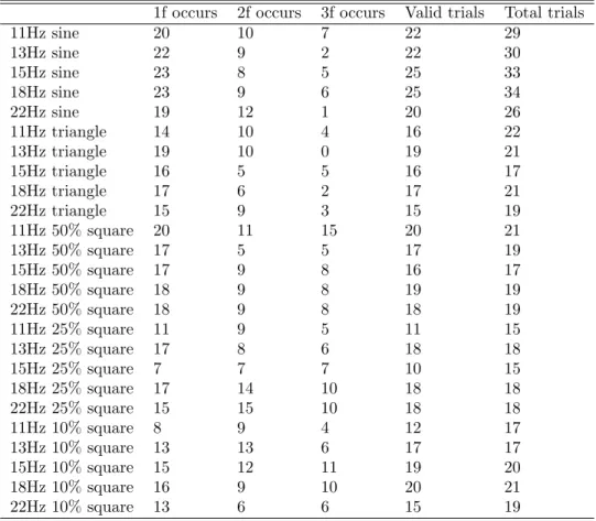
Table 3.1 reports the SSVEP results from all subjects. f is the funda-mental frequency of the stimulus. “Valid trials” is the number of trials that the magnitude of FFT coefficients of SSVEP at f, 2f, or 3f are 50% greater than the baseline. “Total trials” is the number of experiments in which a stimulus is presented to a user, regardless of whether the SSVEP peaks were detected. “1f occurs, 2f occurs, and 3f occurs” are the number of observed SSVEP peaks at 1f, 2f and 3f, respectively.

Theoretically, SSVEP peaks appear at the stimulus frequency 1f and its harmonics 2f, 3f etc. An SSVEP system has to use an recognizable 1f com-ponent to identify which frequency the subject is looking at, while sometimes uses its harmonics to improve the accuracy. Thus, a valid trial without a 1f

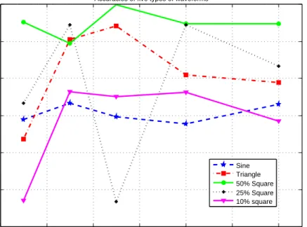
peak may not be acceptable in a real SSVEP system. So we define a trial in which 1f occurs as an accurate trial, and the accuracy of a certain type of waveform of a certain frequency is Accuracywave,f requency = _{T otal trials}1f occurs . Figure 3.2 shows the accuracies of SSVEP trials driven by the three waves above.

Table 3.1: Statistics of harmonics in SSVEP

1f occurs 2f occurs 3f occurs Valid trials Total trials

11Hz sine 20 10 7 22 29 13Hz sine 22 9 2 22 30 15Hz sine 23 8 5 25 33 18Hz sine 23 9 6 25 34 22Hz sine 19 12 1 20 26 11Hz triangle 14 10 4 16 22 13Hz triangle 19 10 0 19 21 15Hz triangle 16 5 5 16 17 18Hz triangle 17 6 2 17 21 22Hz triangle 15 9 3 15 19 11Hz 50% square 20 11 15 20 21 13Hz 50% square 17 5 5 17 19 15Hz 50% square 17 9 8 16 17 18Hz 50% square 18 9 8 19 19 22Hz 50% square 18 9 8 18 19 11Hz 25% square 11 9 5 11 15 13Hz 25% square 17 8 6 18 18 15Hz 25% square 7 7 7 10 15 18Hz 25% square 17 14 10 18 18 22Hz 25% square 15 15 10 18 18 11Hz 10% square 8 9 4 12 17 13Hz 10% square 13 13 6 17 17 15Hz 10% square 15 12 11 19 20 18Hz 10% square 16 9 10 20 21 22Hz 10% square 13 6 6 15 19

We have the following observations.

• A square waves with 50% duty cycle have a significantly higher accuracy than other stimuli in our experiment.

As shown in Figure 3.2, the average accuracies (

P

allf requenciesnumber of accurate trials

P

allf requenciestotal number of trials ) of sine, triangle, and square waves with duty cycle 50%, 25% and 10%

were 70.4%, 81.0%, 94.7%, 79.8%, and 69.1% respectively. Using statis-tic analysis techniques, we check if the performance of 50% square wave is better than that of triangle wave, which is intuitively the second best

10 12 14 16 18 20 22 0.4 0.5 0.6 0.7 0.8 0.9 1 Frequency Accuracy

Accuracies of five types of waveforms

Sine Triangle 50% Square 25% Square 10% square

Figure 3.2: 11, 13, 15, 18 and 22Hz were used as the stimulus frequencies. The accuracies of the SSVEP experiments are computed with equation Accuracy = _{T otal trials}1f occurs .

waveform as seen in Figure 3.2, with a significant level less than 0.05.

90

95 50% square waves and 81

100 triangle waves evoked 1f SSVEP, thus Z = (p1−p2)−(π1−π2) q_p 1(1−p1) n₁ + p₂₍₁−p₂₎ n₂ = 1.728. Since Zα = _σ/x−µ¯ √_n0 = 1.645 < Z, we con-clude that a square waves with 50% duty cycle have a significantly higher accuracy than other stimuli in our experiment.

• A square wave has a higher success rate than sine or triangle waves in eliciting SSVEPs.

In our experiments, the success rates (number of valid trials divided by the total number of trials) for sine, triangle, and square waves were 75.0%, 83.0%, and 90.8%, respectively.

• All three wave forms elicited 2f component in SSVEPs.

In our experiments, the success rates for 2f component in SSVEP were 42.9% for sine waves, 48.2% for triangle waves, and 56.2% for square waves (averaged over all three duty cycles). Among the three duty cycles, 10%, 25%, and 50%, of the square wave, the 2f success rates were 43.0%, 70.7%, and 59.0%, respectively.

• A square wave has a significantly higher success rate than sine or triangle wave in eliciting 3f component in SSVEPs.

In our experiments, the success rates for 3f component in SSVEP were 18.4% for sine waves, 14.0% for triangle waves and 48.0% for square waves (averaged over all three duty cycles). Among the three duty cycles, 10%, 25%, and 50%, of the square wave, the 3f success rates were 44.6%, 50.7%, and 55.0%, respectively.

Although sine, triangle, and square waves with 50% duty cycle do not contain 2f component, they all elicited 2f in SSVEP with similar success rates. Square wave with 25% duty cycle contains a strong 2f component. Its 2f success rate is significantly higher (70.7%). This suggests that: (1) the 2f component is primarily elicited by the fundamental frequency; (2) 8 in the stimuli increase the success rate of 2f in SSVEP. A similar observation is obtained for 3f. This seems to suggest that although the fundamental

frequency can elicit harmonics (2f and 3f in our experiments) in SSVEP, the success rate of getting harmonics in SSVEPs is positively correlated with the strength of the artifacts in a stimulus.

We observed that square waves with 50% duty cycle have a significantly higher accuracy than other stimuli in our experiment. As a result, the use of square waves with 50% duty cycle is preferred if high 1f SSVEP eliciting rate is the goal, while sine waves for SSVEP simulation should be chosen if few harmonic artifacts are wanted.

Our results also show that the harmonics associated with SSVEP are elicited both by the fundamental frequency and the artifacts of the stim-uli, with the 2f component produced by the fundamental frequency and the 3f by the artifacts of square waves. At the same time, SSVEP elicited with square waves do not always contain all the artifactual frequency components, e.g. 3f, and SSVEP with sine waves may have 3f harmonics, which is not a part of the stimuli artifacts.

Chapter 4

DUAL AND TRI-STIMULI

According to Equation 1.1, it is straightforward that the more the possible selections, the more bits (information) a decision carries. Thus, after an effective stimulus, a stimulation method that provides more distinguishable stimuli is the second aspect enhancing the performance of an SSVEP BCI. In this chapter, we propose dual stimuli as the solution, and claim that 4Hz is the resolution1 of the dual stimuli.

4.1

Methodology

Because the strongest SSVEP responses are observed in the range of 5– 20Hz (34; 47; 68), our SSVEP BCI uses 10-20 integer Hz signals as stimuli. Theoretically, SSVEP occurs at exactly the same frequency as a stimulus. However, considering noises from the outside world, an error margin has to be introduced. In our system, we only use integer Hz stimuli between ten to twenty Hz, and round any SSVEP peak (in the frequency domain) between

1_{The resolution is defined as the minimum distance between two frequencies in a dual-stimulus that elicits} consistent SSVEP

[n−0.5, n+0.5) Hz, n=10..20, to n. Under this scenario, one round of SSVEP detection can only make one ”one out of eleven” choice. In order to increase the information throughput, the use of dual stimuli is proposed. Dual stimuli increase the number of distinct stimuli. For example, the sum of 13Hz and 17Hz sine waves is considered a dual stimuli, while the sum of 13Hz and 18Hz sine waves is considered another dual stimuli. Cheng et al. (34) used multiple color stimuli to deliver two stimuli simultaneously. However, no research has been done regarding the resolution of the dual stimuli. This section identifies the resolution of dual stimuli that provides consistent SSVEP. Stimuli were generated by summation of two sine waves on an LED.

Compared with a sine wave, which has no harmonics, a square wave and a triangle wave contain strong harmonic components as given by their Fourier representation. This suggests that the use of sine waves for SSVEP simulation may be preferred over the other wave forms due to reduced harmonic artifacts. In order to make an LED emit a sine wave light signal, a carefully selected DC bias has to be added to the sine input signal. For the LED used in our experiments, the linear region is 3v to 3.5v with DC bias 3.25v.

We tested the dual and tri-stimuli on one human subject. An LED stim-ulator was used to elicit an SSVEP response. For the LED used in our experiments, the linear region is 3v to 3.5v with DC bias 3.25v.

0 5 10 15 20 25 30 35 40 0 1000 2000 3000 4000 5000 6000 7000 |Y| Frequency (Hz) Channel 1 0 5 10 15 20 25 30 35 40 0 1000 2000 3000 4000 5000 6000 7000 |Y| Frequency (Hz) Channel 1

(a) Dual sine stimulus at 11Hz and 17Hz. (b) Dual sine stimulus at 13Hz and 17Hz.

0 5 10 15 20 25 30 35 40 0 1000 2000 3000 4000 5000 6000 7000 8000 9000 10000 |Y| Frequency (Hz) Channel 1 0 5 10 15 20 25 30 35 40 0 1000 2000 3000 4000 5000 6000 7000 8000 |Y| Frequency (Hz) Channel 1

(c) Dual sine stimulus at 15Hz and 17Hz. (d) Dual sine stimulus at 11Hz and 19Hz.

Figure 4.1: Spectrums of SSVEP for dual stimuli.

4.2

Results and Conclusions

We tested the dual stimulus on one human subject. An LED stimulator was used to elicit SSVEP. Five seconds of EEG signal were recorded in each

0 5 10 15 20 25 30 35 40 0 1000 2000 3000 4000 5000 6000 7000 8000 9000 |Y| Frequency (Hz) Channel 1

(a) Tri sine stimulus at 11Hz, 15Hz, 19Hz, Test 1.

0 5 10 15 20 25 30 35 40 0 1000 2000 3000 4000 5000 6000 7000 8000 9000 |Y| Frequency (Hz) Channel 1

(b) Tri sine stimulus at 11Hz, 15Hz, 19Hz, Test 2.

Figure 4.2: Spectrums of SSVEP for tri stimuli.

test. Figure 4.1 shows the spectrum of SSVEP for dual stimulus tests with frequency combination of 11-17Hz, 13-17Hz, 15-17Hz and 11-19Hz. It was observed when the two frequencies in the stimulus were only 2Hz or less apart, SSVEP can only detect one stimulus frequency (Figure 4.1(c)). In most cases, the detected frequency is the lower frequency in the stimulus. Noticeable dual SSVEP spikes could be seen if two frequencies were 4 Hz apart (Figure 4.1(b)), while in most cases, the amplitude of the higher frequency in SSVEP is lower than that of the lower frequency. Two distinctive spikes can be detected if the frequencies of the stimulus were at least 6 Hz apart (Figure 4.1(a)(b)).

For the tri-stimulus tests, we saw three noticeable SSVEP spikes in only one out of five tests (Figure 4.2(b)). In the other four tests, there were spikes at one or two of the three stimulus frequencies. Figure 4.2 shows the results

Table 4.1: SSVEP at different combinations of stimulus frequencies.

Stimulus Number Good Fair Failed Frequencies of Tests Responses Responses Responses

11-13Hz 3 0 0 3 11-15Hz 5 3 1 1 11-17Hz 3 3 0 0 11-19Hz 3 3 0 0 13-19Hz 3 3 0 0 15-19Hz 5 1 1 3 11-15-19Hz 5 1 3 1

of two tri stimulus tests with 11-15-19Hz visual stimuli. It is interesting to observe that in all five tests the lowest frequency was lost in the EEG spectrum instead of the largest frequency as in the dual stimulus tests.

The SSVEP results for different dual- and tri-frequency combinations are summarized in Table 4.1. A “Good response” is one in which all stimulus frequencies are distinctive in SSVEP. A “Fair response” is one in which some stimulus frequencies are distinctive in SSVEP. When there is no SSVEP, we call it a “Failure”.

Chapter 5

STIMULI AND COLOR-SPACE DECOMPOSITION

A good SSVEP system shall focus not only on the usability and speed, but also the user experience. Because the best stimulation frequency region of an SSVEP BCI is 5–20Hz, which reside in the low frequencies (< 30 Hz) range that may cause safety hazards linked to photo-induced epileptic seizures (46; 47), we explore the design of a visually friendly stimulus from the perspective of color-space decomposition in this chapter. This low-frequency visually friendly stimulus is designed with a fixed luminance component and variations in the other two dimensions in the HSL space, based on the assumption that iso-luminant stimuli may ease the feeling of dizziness.

5.1

Methodology

We designed iso-luminant stimuli in the HSL color space. Because the SSVEP has the same fundamental frequency as the visual stimulus (17), it is important to ensure that the stimulators are exact as the software generator set it; otherwise accurate results may not be achieved. In our experiments, the stimuli were carefully designed to achieve credible results, described below.

• Accurate Frequencies

It is not straightforward to deliver accurate stimuli with computer screens. Jaganathan claimed that the PC hardware and operating system seem to determine the variability of stimulation frequency (62). Sugiarto and Sutoyo claimed that DirectX, OpenGL and Matlab are effective in im-plementing an accurate stimulus with a computer screen (123; 124). The refresh rate of the monitor also limits the frequency rage of the stimulus. The refresh rate R is the number of times a display’s image is repainted or refreshed per second. Intuitively, as at least two points form a cycle, only frequencies lower than R/2 Hz can be used and only the subhar-monics of the screen refresh rate can be obtained. Furthermore, the task scheduling that most operating systems perform often affects the render-ing of the frequency, which are usually unpredictably delayed, especially when a lot of stimuli were set simultaneously. Thus, we used DirectX and a CRT monitor with a refresh rate of 60Hz and 120Hz to deliver 6Hz and 12Hz stimuli, respectively. And the program only shows one flashing object on the screen at a time.

• Stimuli

The HSL stimulus was designed as a flashing square box with changing color, sized 100*100 pixels in a 17inch monitor, with a resolution of

Table 5.1: HSL Space Stimuli HSL and RGB Values in One Cycle

Two points Circle “8” size

HSL RGB HSL RGB HSL RGB 1 0.12,0.56,0.80 208,200,200 0.82,0.20,0.80 219,190,189 0.86,0.86,0.80 248,161,160 2 0.12,0.56,0.80 208,200,200 0.72,0.23,0.80 216,193,192 0.80,0.95,0.80 252,157,156 3 0.12,0.56,0.80 208,200,200 0.56,0.24,0.80 216,192,192 0.71,0.86,0.80 248,161,160 4 0.12,0.56,0.80 208,200,200 0.50,0.31,0.80 220,188,188 0.79,0.78,0.80 244,165,164 5 0.12,0.56,0.80 208,200,200 0.47,0.41,0.80 225,183,183 0.69,0.70,0.80 240,169,168 6 1.28,0.87,0.80 233,176,175 0.50,0.53,0.80 231,177,177 0.67,0.53,0.80 231,177,177 7 1.28,0.87,0.80 233,176,175 0.58,0.59,0.80 234,174,174 0.77,0.45,0.80 227,181,181 8 1.28,0.87,0.80 233,176,175 0.74,0.60,0.80 235,174,173 0.89,0.53,0.80 231,178,177 9 1.28,0.87,0.80 233,176,175 0.82,0.52,0.80 231,178,177 0.90,0.69,0.80 239,170,169 10 1.28,0.87,0.80 233,176,175 0.85,0.40,0.80 224,184,184 0.79,0.78,0.80 244,165,164

1024*768 pixels. Three typical HSL-space stimuli were tested, one for a cycle formed by two points jumping between each other, one for a circle and one for a size of number eight. Trajectories and frequency analysis of two of them are shown in Figure 5.1. HSL and RGB values (10 sample points per cycle1) within one cycle are shown in Table 5.1. They have a fixed luminance component and variations in the other two dimensions in the HSL space. Furthermore, it is noteworthy that any frequency could be embedded in HSL stimuli by adding them to either H or S axis. For example, if 11,15 and 18Hz are wanted, we could use

sin(2π ∗11 ∗t) + sin(2π ∗15∗t) as H values and sin(2π ∗18∗t) as S values.

Hue

Saturation

(a) A stimulus with a “circle” trajectory.

Hue

Saturation (b) A stimulus with a “8” shaped trajec-tory. 0 5 10 15 20 25 30 0 10 20 30 40 50 60 70 Amplitude Frequency (Hz) on axis H Circle

(c) Frequencies embedded in the H compo-nent of the “circle” stimulus.

0 5 10 15 20 25 30 0 10 20 30 40 50 60 70 Amplitude Frequency (Hz) on axis H 8

(d) Frequencies embedded in the H compo-nent of the “8” stimulus.

0 5 10 15 20 25 30 0 10 20 30 40 50 60 70 Amplitude Frequency (Hz) on axis S Circle

(e) Frequencies embedded in the S compo-nent of the “circle” stimulus.

0 5 10 15 20 25 30 0 10 20 30 40 50 60 70 Amplitude Frequency (Hz) on axis S 8

(f) Frequencies embedded in the S compo-nent of the “8” stimulus.

Figure 5.1: In the HSL color-space, the luminance is fixed, while the hue and the saturation vary along a trajectory. Frequencies are delivered by the change of the Hue and Saturation together

5.2

Results and Conclusions

Six subjects participated in this experiment. EEG was recorded with one channel over the occipital cortex at a sampling rate of 1kHz, filtered by a 0.15Hz high-pass filter and a 150Hz low-pass filter. The resistances between the skin and the sensor are all below 10k. The distance between the CRT and a subject was 40 cm. We examined stimuli of 6Hz and 12Hz, and recorded the SSVEPs of “two points”, circle, “‘8” shaped trajectory and a black-white flashing box as the control stimuli. This test session was repeated for three times. In each recording session, the subject was told to look at the stimulus for 10 seconds and close their eyes for a rest period of a random duration from 10 to 20 seconds. The recorded data were discarded then repeated when muscle movements artifacts were significant. Figure 5.2 shows the SSVEP spectrums of the above four stimuli.

The primary research goals of these experiments are to find out if these stimuli elicit SSVEP, and if this color-space decomposition makes low-frequency stimuli more visually friendly than ordinary luminance stimuli. Table 5.2 re-ports the SSVEP results of all subjects. f is the fundamental frequency of the stimulus. “Total trials” is the number of experiments in which a stimulus is presented to a user. “1f occurs, 2f occurs” are the number of observed SSVEP peaks at 1f and 2f.

Figure 5.2: Spectrums of SSVEP of three types of stimulation. The stimulus is a 12Hz flashing square on a computer screen.

Table 5.2: Statistic of harmonics in SSVEP

1f occurs 2f occurs Total trials 6Hz two pints 18 10 18 6Hz circle 18 11 18 6Hz eight 18 15 18 6Hz control 18 18 18 12Hz two points 18 10 18 12Hz circle 18 12 18 12Hz eight 18 15 18 12Hz control 18 18 18

• A stimulus with a fixed luminance and variations in the other two di-mensions in the HSL space elicits SSVEP.

As shown in Table 3.1, all HSL space stimuli elicit SSVEP at their fun-damental frequency.

• The embedded frequencies affect SSVEP.

In our experiments, the success rates (number of its occurrence divided by the total number of trials) of “2f occurs” for two points, circle and “8” stimuli were 55.6%, 63.9%, and 83.3%, respectively, which suggests that the embedded 2f in “8” stimulus affects the 2f harmonic in its SSVEP.

• All stimuli elicit SSVEP harmonics.

All types of stimuli evoke harmonics, though the success rates vary. • This color-space decomposition makes low-frequency stimuli more

visu-ally friendly than ordinary luminance stimuli.

All six subjects felt these fixed luminance stimuli were more comfortable than the control “black-white flashing box” stimulus. However, there is not enough evidence to conclude that this technique decreases the risk of safety hazards.

Chapter 6

POTENTIAL FUNCTION CLASSIFIER

A machine learning approach introduces adaptiveness, accuracy and speed to an SSVEP BCI, and improves BCI performance by learning brain patterns. Considering that a subject’s brain signal is non-stationary, e.g., the SSVEP responds may be strong in the morning but weak in the afternoon, a simple threshold may not be a good choice: if it is set too high, it will miss peaks in the afternoon, if it is set too low, it will categorize noises as SSVEP. Con-sequently, Potential Function Classifier (PFR) is introduced to our SSVEP BCI.

The PFR is motivated by the potential field of static electricity. A binary PFR views each training sample as an electrical charge, positive or negative according to its class label. The resulting potential field divides the feature space into two decision regions based on the polarity of the potential. The ba-sic idea of binary PFRs can be generalized to the multiclass scenario, in which a potential function is defined for each class using the training observations within that class. A new observation is then assigned a label corresponding to

the class of the highest potential value. Intuitively, adding new classes does not affect the existing potential functions. Removing or merging classes influ-ence only the potential functions of the classes involved in the operation. In SSVEP-based BCI context, these advantages can be interpreted as: Adding a new stimulus do not affect the existing PFRs. Removing a stimulus that is not currently well responded or merging stimuli that are not clearly separable influence only the PFRs involved in the operation. This good scalability of PFRs makes it suitable to BCI systems.

In this chapter, we first introduce the PFR method from the perspective of a machine learning technique. Then run PFR in offline SSVEP data and compare its bit rate calculated by Eq.(1.1) as the comparison metric.

6.1

Introduction

For thousands of years, various civilizations have observed “static electric-ity” where pieces of small objects with the same kind of electricity repelled each other and pieces with the opposite kind attracted each other. potential function rules were motivated from the underlying property of static electric-ity to predict the unknown binary nature of an observation, a problem com-monly known as binary classification. Potential function rules were originally studied by Aizerman, Braverman, Rozonoer, and several other researchers in the 1960’s ((2; 3; 12; 27; 28)). In its simplest form, a potential function rule

puts a unit of positive electrical charge at every positive observation and a unit of negative electrical charge at every negative observation. The resulting potential field defines an intuitively appealing classifier: a new observation is predicted positive if the potential at that location is positive, and negative if its potential is negative.

Below, we revisit potential function rules (PFRs) in their original form and reveal their connections with other well-known results in the literature. We derive a bound on the generalization performance of potential function classifiers based on the observed margin distribution of the training data. A new model selection criterion using a normalized margin distribution is then proposed to learn “good” potential function classifiers in practice.

6.2

Background

There is an abundance of prior work in the field of pattern recognition and machine learning. It is beyond the scope of this study to supply a complete review of the area (for more comprehensive surveys on various subjects, the reader is referred to Devroye et al. (40), Duda et al. (44), Bishop (20) for patter recognition, to Sch¨olkopf and Smola (116), Shawe-Taylor and Cris-tianini (119) for kernel methods, to Anthony and Biggs (5), Kearns and Vazirani (66) for computational learning theory, and to Mitchell (87), Hastie et al. (58), Vapnik (131) for machine/statistical learning). Nevertheless, a

brief synopsis of some of the main findings will serve to provide a rationale for the proposal of a new machine learning approach used in an SSVEP BCI. A multiclass classification problem aims at foretelling the unknown nature of an observation. More formally, an observation is a d-dimensional vector of numerical measurements denoted as x ∈ _Rd_{. The unknown nature of the} observation, z, takes values in a finite set _K = {1,2, . . . , K}, the set of class labels. A mapping f : _Rd → _K, which is named a classifier, predicts the class label of an observation.

Does there exist an “optimal” classifier for a given classification task? Under a probabilistic setting, the Bayesian decision theory (13; 15) gives an affirmative answer – the Bayes decision rule (called the Bayes classifier). If the pair of observations and their nature, (x, z), is a random variable with a joint probability distribution p(x, z), the Bayes classifier, f∗, selects the class label for an observationxasf∗(x) = argmax_z∈KPr(z|x) = argmax_z∈Kp(x, z). The optimality of f∗ is defined by the minimum probability of error, i.e., Pr[f∗(x) 6= z] ≤ Pr[f(x) 6= z] for any f : _Rd → _K, which is well-known as the Bayesian probability of error. This probability measures the ‘hardness’ of a classification problem. It can theoretically be evaluated if the joint distribution is known, but the calculation may be (and usually is) intractable in practice due to the min operator inside of the integral. Several tight

bounds are proposed in the literature for computational approximations of the Bayesian probability of error (38; 57; 7).

The crux of the Bayesian approach is the difficulty of determining the joint distribution. Plug-in decision (40) is a natural way of applying the Bayesian classification in practice, where an approximated Bayes classifier is constructed using an estimated joint distribution. Depending upon the way in which the joint distribution is estimated, plug-in decision rules fall roughly into parametric approaches and nonparametric approaches.

In a parametric approach, the unknown joint distribution is described by a set of parameters based on certain structural assumptions, e.g., conditional independence of attributes within each class (75; 41; 26), mixture of Gaus-sians (69; 122), and mixture of Bernoullis (122). The values of the param-eters are obtained by optimizing a loss function, e.g., a likelihood function. In many applications, a parametric approach presents an efficient means of incorporating prior knowledge about the data. For example, Hofmann et al. (61) used a latent variable model (aspect model) to remove the statisti-cal dependence among words in a document for textual data. Barnard et al. (9) explored several generative models to describe statistical relevance be-tween image regions and associated texts. Veeramachaneni and Nagy (133) studied the interpattern dependence, named style context, for Optical

Char-acter Recognition. Intraclass style (statistical dependence between patterns of the same class in a field) and interclass style (statistical dependence be-tween patterns of different classes in the same field) were formalized to derive style-constrained Bayesian classification.

The performance of a plug-in decision rule is determined by the quality of the estimated joint distribution. Ben-Bassat et al. analyzed the sensitivity of Bayesian classification under multiplicative perturbation on the joint dis-tribution. Devroye (39) presented a more general result showing that if the estimated posterior probability is close to the true posterior probability inL1

-sense, the error probability of the plug-in decision rule is near the Bayesian probability of error. Nevertheless, does the error probability converge to the Bayesian probability of error if more training samples are obtained to approximate an arbitrary joint distribution? This is a question regarding the universal consistency of a classification rule. Loosely speaking, a uni-versally consistent rule (40) guarantees us that taking more samples suffices to roughly reconstruct an arbitrary, fixed, but unknown distribution, hence to asymptotically achieve the optimality. While parametric approaches are efficient, in general they are not universally consistent.

In 1977, Stone proved the existence of a universally consistent rule (121). He showed that any k-nearest neighbor classifier is universally consistent if