Clock Synchronization for Multihop Wireless Sensor Networks

CLOCK SYNCHRONIZATION FOR MULTIHOP WIRELESS SENSOR NETWORKS

BY

ROBERTO SOLIS ROBLES

Ingen, Instituto Tecnologico de Zacatecas, 1992

Maest, Instituto Tecnologico y de Estudios Superiores de Monterrey, 1999

DISSERTATION

Submitted in partial fulfillment of the requirements for the degree of Doctor of Philosophy in Computer Science

in the Graduate College of the

University of Illinois at Urbana-Champaign, 2009

Urbana, Illinois Doctoral Committee:

Professor P. R. Kumar, Chair and Director of Research Professor Lui Sha

Professor Carl A. Gunter

UMI Number: 3392480

All rights reserved

INFORMATION TO ALL USERS

The quality of this reproduction is dependent upon the quality of the copy submitted. In the unlikely event that the author did not send a complete manuscript and there are missing pages, these will be noted. Also, if material had to be removed,

a note will indicate the deletion.

UMI

Dissertation Publishing

UMI 3392480

Copyright 2010 by ProQuest LLC.

All rights reserved. This edition of the work is protected against unauthorized copying under Title 17, United States Code.

uest

ProQuest LLC

789 East Eisenhower Parkway P.O. Box 1346

A B S T R A C T

In wireless sensor networks, more so generally than in other types of distributed systems, clock synchronization is crucial since by having this service available, several applications such as media access protocols, object tracking, or data fusion, would improve their performance. In this dissertation, we propose a set of algorithms to achieve accurate time synchronization in large multihop wireless networks.

First, we present a fully distributed and asynchronous algorithm that has been designed to exploit the large number of global constraints that have to be satisfied by a common notion of time in a multihop network. For example, the sum of the clock offsets along any cycle in the network must be zero at any instant. This leads to the concept of "spatial smoothing." By imposing the large number of global constraints for all the cycles in the multihop network, these time estimates can be smoothed and made more accurate.

The algorithm functions by simple asynchronous broadcasts at each node. Chang-ing the time reference node for synchronization is also easy, consistChang-ing simply of one node switching on adaptation, and another switching it off. It has been implemented on a Berkeley motes testbed of forty nodes, and comparative evaluation against a leading algorithm is presented.

Next, considering that most of the clock synchronization protocols that have been developed do not provide means to detect security attacks which could render them useless, we present a secure network-wide clock synchronization protocol. At the same time, this protocol allows the nodes to securely discover the network's topology by

detecting and isolating all links that have fallen under the control of attackers. The protocol detects the attacks using only timing information under certain conditions. It has been implemented on an IMote2 testbed of twenty five nodes. Experimental results are provided.

A C K N O W L E D G M E N T S

This dissertation would not have been possible without the help, encouragement, and support of many people.

I am specially grateful to my adviser, Professor P. R. Kumar, for his guidance and continued support throughout the years. Without him, this work would have not been possible. I thank the members of my Ph.D. committe, Professors Lui Sha, Carl Gunter and Yih-Chun Hu for their invaluable comments and suggestions to improve this dissertation. I would also like to thank the staff of the Coordinated Science Laboratory and all my friends and colleagues there.

I want to acknowledge the financial support received from Instituto Tecnologico de Zacatecas, Universidad Autonoma de Zacatecas, Fulbright-CONACYT, PROMEP, and Professor P. R. Kumar, which allowed me in one time or the other, to complete this dissertation.

Finally, thanks to my parents, Honoria and Rufino, for always being there for me, and specially to Sahara, my wife, who endured this long journey, and has given me the joy of two beautiful children, Sahara and Alberto; they all have made it worth the effort.

TABLE OF C O N T E N T S

LIST OF FIGURES ix C H A P T E R 1 I N T R O D U C T I O N 1

1.1 Wireless Sensor Networks 1 1.2 Importance of Clock Synchronization 2

C H A P T E R 2 MOTIVATION A N D RELATED W O R K 5

2.1 Virtual Clocks 6 2.2 Theoretical Results 7 2.3 General Network Algorithms 8

2.4 Ad Hoc Networks 10 2.5 Wireless Sensor Networks 11

2.5.1 Sources of error in the clock synchronization process 11

2.5.2 Berkeley motes and TinyOS 12 2.5.3 Reference broadcast synchronization (RBS) 14

2.5.4 Tiny-sync and mini-sync 16 2.5.5 Timing-sync protocol for sensor networks (TPSN) 17

2.5.6 Flooding time synchronization protocol (FTSP) 19 2.5.7 Lightweight tree-based synchronization (LTS) 20

2.5.8 Adaptive clock synchronization 20 2.5.9 Pairwise broadcast synchronization (PBS) 21

2.5.10 Gradient time synchronization protocol (GTSP) 21 2.5.11 Average time sync (ATS) . 21

C H A P T E R 3 BILATERAL CLOCK SYNCHRONIZATION

ALGORITHM 23

3.1 System Model 23 3.2 Pair-wise Clock Synchronization between Neighbors 23

3.3 Simulation Results 30 3.4 Implementation on Berkeley Motes 31

3.4.1 Setup 33 3.5 Evaluation 34

C H A P T E R 4 MULTIHOP CLOCK SYNCHRONIZATION . . . . 36

4.1 Formulation 37 4.2 Implementation on Berkeley Motes 44

4.2.1 Setup 44 4.3 Evaluation 45

C H A P T E R 5 SECURITY A N D CLOCK SYNCHRONIZATION . 48

5.1 Requirements for Sensor Network Security 49

5.2 Attacks 49 5.3 Defenses 51 5.4 Secure Clock Synchronization 53

5.4.1 SPS and SGS 54 5.4.2 Secure and resilient clock synchronization 54

C H A P T E R 6 SECURE CLOCK SYNCHRONIZATION OVER A

SINGLE LINK 55

6.1 Protocol Description 55 6.1.1 Notation 55 6.1.2 Assumptions 56 6.1.3 Basic clock synchronization protocol 57

6.1.4 Adding security to the protocol 59

6.2 Implementation . 64 6.2.1 Exponential smoothing 65

6.2.2 MAC layer timestamping 66 6.2.3 Neighbor discovery subprotocol 68

6.3 Evaluation 70 6.3.1 Clock synchronization 70

6.3.2 Validation of clock synchronization 71

6.3.3 Man-in-the-middle attacker 73

6.4 Security Analysis 79 6.4.1 Consistent skew 79 6.4.2 Consistent one-way delay 80

6.4.3 Security of delayed authentication 81 6.4.4 Security against inter-session replay 82

C H A P T E R 7 SECURE N E T W O R K - W I D E CLOCK

SYNCHRONIZATION A N D TOPOLOGY DISCOVERY 84

7.1 The Main Ideas 86 7.1.1 Single link checking 86

7.1.2 Neighborhood check 87 7.1.3 Network consistency check 87 7.1.4 Removal of network inconsistencies 89

7.1.5 An example 90 7.2 Implementation 97

7.2.2 Exchange of valid neighbor lists 98 7.2.3 Exchange of reachable lists 99 7.2.4 Removal of network inconsistencies 101

7.3 Evaluation 101

C H A P T E R 8 CONCLUSIONS A N D F U T U R E WORK 106

8.1 Future Work 107

R E F E R E N C E S 108 AUTHOR'S B I O G R A P H Y 118

LIST OF FIGURES

2.1 Relationship between the various levels of NTP 9 2.2 Illustration of the sources of error during clock synchronization. . . . 12

2.3 Illustration of two places where the timestamping can be performed. . 13 2.4 Exchange of messages to determine relative drift and offset between

two nodes 16 2.5 Two-way message exchange 19

3.1 Frequent transmissions of estimates to neighbor node 24

3.2 Skew estimation results obtained in simulation 30 3.3 Offset estimation results obtained in simulation 31

3.4 Communication stack on TinyOS 1.x 32 3.5 Implementation setup for two nodes 33 3.6 Accuracy of estimated to real time between 2 neighboring nodes. . . . 35

4.1 Example of a network 38 4.2 Link topology for the multihop implementation 45

4.3 Average closeness of estimated to real time in a 40-node network. . . 46

4.4 Experimental results of FTSP on the 40-node network 46

4.5 Comparison to FTSP 47 6.1 Message exchanges to achieve basic clock synchronization 58

6.2 Detecting a half-duplex attacker. Source: [1] 62 6.3 Illustration of MAC layer timestamping in the CC2420 radio 67

6.4 Linear skew 72 6.5 Accuracy of packet arrival time prediction and RTT behavior 72

6.6 CDF of the errors in the arrival time prediction 73 6.7 Experimental setup with an MITM attacker 74 6.8 Skews observed with an MITM attacker present 75 6.9 Comparison of skews with no MITM and with MITM 76

6.10 Round-trip time observed with MITM present 76 6.11 Accuracy of packet arrival time prediction with MITM present . . . . 77

7.1 Example network to illustrate secure multihop protocol execution . . 90

7.2 Neighborhood check step in nodes 3 and 5 92 7.3 Lists of neighbors received in node 7 92

7.4 Node 7 exchanges its reachable list with its neighbors 93 7.5 Node 7 receives reachable lists from its neighbors 94 7.6 Node 7 exchanges its reachable list with neighbors again 95

7.7 Node 7 wants to communicate with node 1 but needs to first remove

the inconsistencies 96 7.8 Testbed for the implementation of the secure network-wide

synchro-nization protocol 98 7.9 Link topology of the 25 nodes in the testbed 99

7.10 Skews observed by node 1 in a particular run of the experiment. . . . 104 7.11 Skews observed by node 13 in a particular run of the experiment. . . 104 7.12 Skews observed by node 22 in a particular run of the experiment. . . 105

C H A P T E R 1

I N T R O D U C T I O N

1.1 Wireless Sensor Networks

Technological advances made in recent years in the fields of microelectronics and wireless communications have enabled the integration of sensors, actuators and ra-dios, which has lead to the development and deployment of wireless sensor networks. Wireless sensor networks have grown in popularity and the applications that can be developed for such networks are widespread, ranging from target tracking surveil-lance [2,3], to biomedical health monitoring [4] and seismic sensing [5]. Along with these applications come new design challenges [6,7], which stem from the fact that a wireless sensor network has limited resources in terms of memory, computation power, bandwidth and energy; and design constraints based on the monitored envi-ronment. These play a key role in determining many aspects of the network such as size, deployment scheme and topology. For example, in terms of resource constraints, the MICA2 Berkeley motes [8] use an 8-bit micro-controller running at 4 MHz with a limited instruction set, have only 4KB of RAM memory and can transmit up to 19.2 kbps. They are battery powered by an inexpensive pair of AA batteries that produce between 2.0 and 3.2 V, and the lifetime is mainly determined by its awake duty-cycle and radio usage.

1.2 Importance of Clock Synchronization

For several distributed applications either it is necessary for the processors to have a common notion of time, or to have it would improve their performance. Examples of these applications are authentication protocols, media access protocols, and database consistency [9]. In the case of wireless sensor networks, applications such as object tracking, environmental monitoring, TDMA scheduling, and data fusion, require some kind of timing service in order to determine the order in which events have unfolded and also the actual times of the events themselves. The synchronization would also allow the nodes to save energy. In wireless sensor networks, the accuracy of object localization or tracking is limited by the accuracy of clock synchronization [10]. When actuation is also performed over the network, accurate clock synchronization is needed to avoid delay induced instabilities, and improve control system performance [11]. Due to its importance, several algorithms have therefore been designed ( [12-30]) in order to synchronize the clocks of a distributed system over traditional networks, and also over wireless sensor networks.

In this dissertation, two algorithms to achieve clock synchronization in a multihop wireless sensor network are presented as well as the results on their performance in implementations.

For the first algorithm, the key novelty of the approach presented consists of a new notion of "spatial smoothing." It exploits global constraints imposed by a common notion of time to improve the performance of clock synchronization, and yet achieves this through a completely asynchronous, distributed algorithm. The heart of the idea is the following. Suppose Oy is the offset of the clock at node j with respect to the clock at a neighboring node i, at a certain time. Then an estimate of Oij can be formed by bilateral exchange (or broadcast) of timestamped packets between the neighboring nodes i and j . These estimates are, however, noisy and

are based only on the particular timestamped packets exchanged between the two neighboring nodes. Now consider any cycle formed by nodes ii, i2,.. •, in, in+i = H,

in the multihop network. Necessarily, Y^=i ^ikik+1 = 0 must be satisfied by the very

notion of common time. This is an example of one global constraint, and there are several such global constraints, one for every cycle in the graph. By taking advantage of these constraints, the noisy estimates Oij can be further smoothed to give better estimates. Imposing these global constraints can thus improve the time estimate at every node in a multihop network with respect to any chosen reference node. Essentially, this procedure allows full exploitation of all bilateral estimates, i.e., all global information, to synchronize the clock at every node, thus making possible the spatial smoothing of otherwise noisy local time estimates.

Thus we obtain a completely distributed asynchronous algorithm, where nodes communicate only with their neighboring nodes, to achieve these global constraints. Our distributed algorithm takes advantage of all estimates of bilateral offsets all over the network to improve performance at every node, and not just those, say, along a rooted tree. The incorporation of such a large number of global constraints improves clock synchronization, especially in large networks where there are indeed a large number of such constraints.

As noted above, this algorithm does not require any constructions such as a rooted tree. In fact, it does not need any global topology knowledge. Instead it only uses asynchronous distributed broadcasts at each node. Moreover, switching the time reference from one node to another is also easy. It simply consists of one node switching on adaptation, and another switching it off, and the entire network then adapts to the change.

The results of an implementation over a 40-node Berkeley motes testbed and a comparison of these results with a leading clock synchronization protocol on the testbed are presented.

For the second algorithm, security is taken into account and based on theoretical work by Chiang et al. [1], we first develop and implement a secure clock synchroniza-tion protocol over a single link that is able to detect man-in-the-middle attacks using only timing information. In man-in-the-middle attacks, the attacker intercepts mes-sages exchanged between two nodes and relays such mesmes-sages in a way that makes the two nodes believe that the link they share is valid, while in reality the characteristics of the link have been modified. For instance, delays are introduced which could affect the clock synchronization service. By using the secure clock synchronization protocol, nodes are able to impose restrictions on the kind of delays a man-in-the-middle at-tacker can add to the packets exchanged between them. We validate the assumptions and properties of the theoretical protocol by means of an implementation performed using IMote2 motes and TinyOS 2.1. We further proceed to successfully implement a mechanism to detect half-duplex man-in-the-middle attackers.

Finally, the secure clock synchronization protocol is extended to securely synchro-nize the clocks in a multihop network. At the same time this protocol also allows the nodes in the network to securely discover the topology of the network. The ul-timate goal of this secure network-wide clock synchronization protocol is to obtain a network-consistent clock.

This protocol is able to detect misbehaving or compromised links, disseminate information regarding those links and effectively isolate them. It is divided into four steps: single link check, neighborhood check, network consistency check, and removal of network inconsistencies.

The protocol has been implemented on a testbed comprised of 25 Crossbow IMote2 sensor nodes on top of TinyOS 2.1. Experimental results are presented.

C H A P T E R 2

MOTIVATION AND RELATED

W O R K

The applications deployed over wireless sensor networks range from environmental monitoring [5,31-34], health and wellness monitoring [35,36] distributed control [37], and object tracking [10,38], to control over networks [39-41]. Most of these appli-cations need to determine the times of the events that occur during their execution, thus requiring a clock synchronization service.

For instance, in [10], a network of directional sensors is intended to monitor a region which is crossed sporadically by objects assumed to be moving at nearly con-stant velocity. Using the times at which sensors detect objects crossing their "field of vision," the trajectories of the objects can be determined as well as the sensor directions, which are also unknown a priori.

An accurate notion of time can also be used to improve communication network performance. By having nodes in a wireless network synchronized, implementation of MAC protocols such as TDMA or SEEDEX [42] would be feasible. This can lead to greater throughput [43]. In addition, it can also be used to conserve energy by reducing collisions when nodes transmit over the shared medium, as well as sleep while awaiting their turn to transmit. Accurate clock synchronization can allow nodes to more accurately coordinate their sleep states by employing advanced duty-cycling schemes [44].

Clock synchronization has been an important topic of research for several years. Several algorithms have been developed, mainly for traditional wireline networks, and, lately, many for wireless sensor networks. This chapter presents the most important

references in this field beginning with the seminal work by Lamport on virtual clocks, followed by some important theoretical results and the main algorithms proposed for traditional, ad-hoc, and sensor networks.

2.1 Virtual Clocks

The seminal work in clock synchronization is due to Lamport [45], where the idea of virtual clocks is used. In his system, he defines the "happened before" relation (denoted by the symbol —•) as follows:

1. If a and b are events in the same process, and a comes before b, then a —>• b. 2. If a is the sending of a message by one process and b is the receipt of the same

message by another process, then a —> b. 3. If a —» b and b —»• c then a —»• c.

4. Two distinct events a and b are said to be "concurrent" if neither a —> b nor b —>• a hold.

Also, a logical clock Ci is defined as a function that assigns a real number Ci(a) to any event a in that process. The clock meets the following condition: For any events a, b in process i, if a —> 6, then Ci(a) < Q(6) as long as the following holds:

1. If a and b are events in process Pi and a comes before b, then Cj(a) < Ci(b). 2. If a is the sending of a message by process Pi and 6 is the receipt of the same

message by process Pj, then Ci(a) < Cj(b).

Finally, a total ordering "happened before" relation, denoted by => is defined. It extends the —> relation to a total ordering by assigning processors a priority to break the ties. However, the resulting total order is not unique.

This work also determines that in case of physical clocks, the closest that two clocks can get is approximately d(pr + e), where d is the diameter of the network, p is the drift rate of the clock, r is the time interval over which a clock synchronization message is sent, and e is the maximum unpredictable delay of the message.

2.2 Theoretical Results

Several theoretical results have been published regarding clock synchronization, the most important being the following:

• In [46], Dolev and Halpern prove the impossibility of achieving clock synchro-nization if more than a third of the nodes in the network are faulty, and give the requirements to be met in order to achieve it.

• In [47], Lundelius and Lynch show that no algorithm can synchronize clocks exactly, and provide lower and upper bounds on how close the clock values can be at the same real time in a fully connected network.

• In [48], Biaz and Welch provide a lower bound for the optimal clock synchro-nization achievable for any network topology, taking into account the diameter of the network, and provide a tighter bound for a specific class of network topologies.

• In [11], Graham and Kumar show that it is fundamentally impossible to es-timate time between two clocks precisely without assuming symmetric delays. Clock skew can be estimated regardless, and also, after two nodes have clock synchronized, when one node sends a packet to the other, the sender can per-fectly predict the time at which the packet will be received in terms of the receiver's clock.

• In [49], Gurewitz et al. propose a method to estimate the one-way delay for each link in an N-node network that works by summing up all single-hop one-way measurements made along various cyclic paths. They show that the maximal number of independent cyclic path delays that can be computed is smaller than the number of links by N-l, which means that it is not possible to uniquely determine the one-way delays.

• In [50], Freris and Kumar analyze networks of clocks, and characterize what is determinable from what is not.

2.3 General Network Algorithms

The basic idea of a clock synchronization algorithm is that a node has a logical clock which provides a time base for all activities on a node [51], and which is derived from the hardware clock on the node. The algorithm executed can be viewed as a clock process invoked at the end of every resynchronization interval. This process is responsible for periodically reading the clock values at other nodes and then adjusting the corresponding local clock value. The algorithm must satisfy the following two conditions:

1. Agreement: The offset between all non-faulty clocks in the system is bounded. 2. Accuracy: The logical clock keeps up with the real time.

The diverse algorithms differ in the way these conditions are specified and in the way the clock processes read the clock values at the other nodes. They can be divided into two categories:

1. Deterministic: These guarantee an upper bound on the closeness of the synchro-nization attainable, assuming an upper bound on transmission delays [52-55].

2. Probabilistic: These do not make any assumptions about the uncertainty, and provide a smaller expected upper bound on the closeness of synchronization, but do not guarantee such a bound with probability one [56,57].

External

Reference Clock

Stratum 1

Stratum 2

Stratum 3

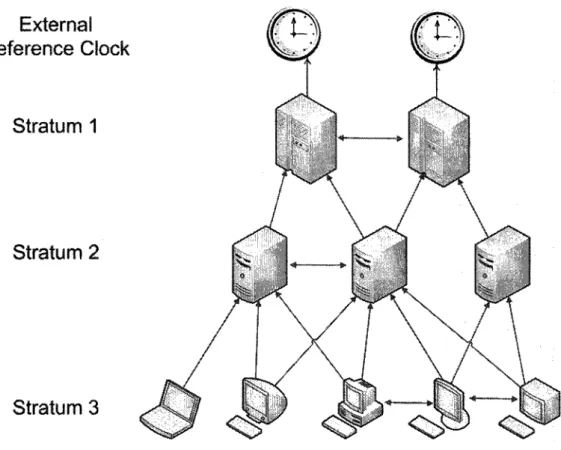
Figure 2.1: Relationship between the various levels of NTP.

One important algorithm which is widely used is the Network Time Protocol (NTP) described in [12]. As can be seen in Figure 2.1, in NTP each group of processes served by the synchronization protocol is organized in a hierarchical structure. The primary servers are located at the root level or stratum 1, and are synchronized to accurate external clocks. Nodes at stratum 2 are synchronized with the primary servers at stratum 1, nodes at stratum 3 are synchronized with nodes at stratum 2, and so on. To withstand possible failures in nodes or network links, nodes at the different strata can obtain time readings from several nodes, resulting in a redundant topology. To achieve synchronization, nodes exchange messages which include the

latest three timestamps that, together with the time at which the message is received, allow estimating round-trip delays and clock offsets. These estimates are then filtered to reduce timing noise, and a peer-selection algorithm is used to determine which subset is the most accurate and reliable. The resulting offsets of this subset are combined using a weighted-average basis, and processed by a phase-lock loop to produce a phase-correction term used to control the local clock. Levels close to the root of the subnet have better accuracy and precision relative to the external standard.

2.4 A d H o c N e t w o r k s

An ad hoc network is a network of mobile wireless computing devices which have a possibly dynamical topology, there being no infrastructure. An algorithm for clock synchronization suitable for ad hoc networks is proposed in [13]. The basic idea of this algorithm is not to synchronize the local clocks of the devices but to generate time stamps using unsynchronized local clocks that when passed between devices will be transformed to the local time of the receiving device. Since these transformations cannot be done with high precision due to the unpredictability of the computer clocks, the algorithm estimates a lower and upper bound for the real time passed from the generation of a timestamp to its arrival in the destination, transforms such bounds to the time of the receiver, and subtracts the resulting values from the time of arrival in the destination node. This results in an interval specifying lower and upper bounds for the time stamp relative to the local time of the receiving node.

The accuracy obtained is in the order of milliseconds for an implementation over a 100 Mbps Ethernet network. A time translation control time protocol is also devel-oped in [11] which is suitable for control applications over networks. It is also shown that it is impossible to synchronize under asymmetric delays, i.e., when

communica-tion delays in the two direccommunica-tions are different.

2.5 Wireless Sensor Networks

For wireless sensor networks which share the limitations of an ad hoc network, along with a need, generally, for greater energy efficiency, a few algorithms have been pro-posed. Before describing the more important algorithms in this area, we review what are the sources of error in the clock synchronization process [14,58], and describe the most common architecture used to implement the algorithms for sensor networks, Berkeley motes [59].

2.5.1 Sources of error in the clock synchronization process

First we define some terminology.

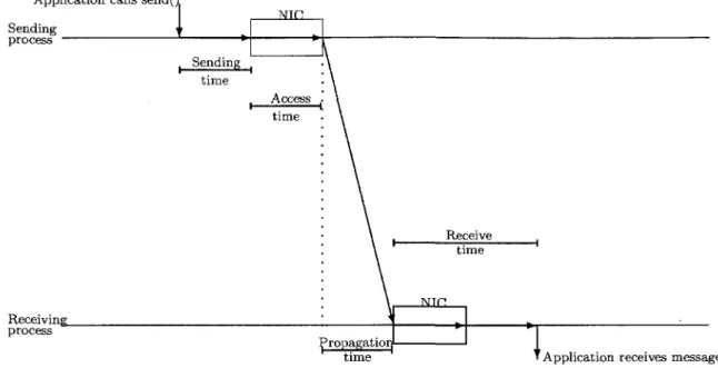
Send time. This is the time spent at the sender to pass the message from the

ap-plication to the network interface.

Access time. This is the delay incurred waiting for access to transmit on the

chan-nel, which in turn is dependent on the MAC protocol being used.

Propagation time. This is the time in transit from the sender to the receiver, once

the message has left the sender. This time is very small on a local network if the sender and receiver share access to the same physical media.

Receive time. This is the time needed to process the message once it has arrived

at the receiver's network interface.

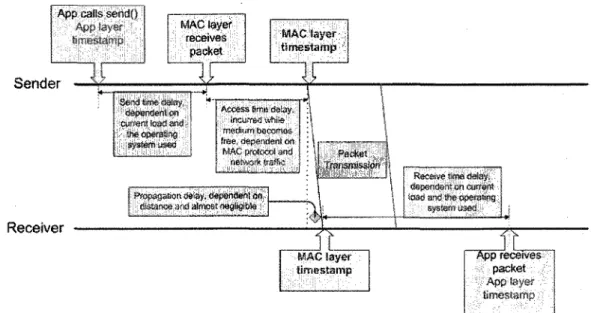
These quantities affect the latencies of communications between nodes, and are shown graphically in Figure 2.2. Figure 2.3 shows the difference between timestamp-ing at the application layer and the MAC layer and how some of sources of error can be avoided.

Application calls send() Sending process Receiving, process t-'ropagationf 1 I

i Application receives message

Figure 2.2: Illustration of the sources of error during clock synchronization.

2.5.2 Berkeley motes and Tiny OS

A mote is an autonomous sensor node which provides a combination of sensing, com-munication and computation, in a complete architecture which has been developed at the University of California, Berkeley [59].

Berkeley motes run the TinyOS Operating System, which is an open-source oper-ating system designed for wireless embedded sensor networks. Its component-based architecture enables rapid implementation while minimizing code size as required by the severe memory constraints inherent in sensor networks [60]. Applications are written in nesC, which is a new language for programming structured component-based applications that has a C-like syntax and supports the TinyOS concurrency model [61].

Over the years, motes architecture has been improved in terms of processing power, memory and communication capabilities. We describe some of the features of three different types of motes to illustrate these improvements (for more details, see [62,63]).

App calis senolO App layer Imestamp MAC layer receives packet Sender MAC layer; timestariii>:

II

Send fee «tey. dependentm current toad and

the operating

Access 8me delay,

incurred wWie mstikm oacomas tee, dependent on

hSAC protocol and

neiwettt traffic

I Pwpagaiwndi^siy. dependent o« I distance and almost n6a,lia.iMe |

i Packet • Transmission

J J Recaye ime delay, dependent on cutram w»d and syswsused T i S T i-M&G. l a y e r ifimestirnp "App receives packet App layer ttmesjsmp

Figure 2.3: Illustration of two places where the timestamping can be performed. at 4 MHz. It has 128 KBytes of onboard flash memory to store the mote's program and 4 KBytes of RAM.

It comes with 512 KBytes of flash memory to hold data, and also has a 10-bit A/D converter so that sensor data can be digitized. Sensors available include temperature, acceleration, light, sound and magnetic. Finally, the radio module consists of an RF Monolithics TR1000 transceiver that can operate at communication rates up to 40 kbps. The complete system is designed to operate off an inexpensive pair of AA batteries that produce between 2.0 and 3.2 V.

A MICA2 mote [8] has similar features as the MICA, but uses a different radio, the Chipcon CC1000, which allows a better range and better noise immunity. It also allows us to program the frequency at which to transmit the data, and has support for wireless remote reprogramming which is very helpful when there is a large number of motes to program. The processor has a 7.3728MHz crystal to support higher UART baud rates.

An IMote2 mote [65], which is a newer generation of mote, uses an Intel PXA271 XScale processor at 13 MHz (scalable up to 416 MHz). It has 256 KB of SRAM and

32 MB of SDRAM. It uses a CC2420 IEEE 802.15.4 radio module which supports a 250 kbps rate with 16 channels in the 2.4 GHz band.

The software side of the architecture, that is, TinyOS, has also been improved over the years [60]. In 2001, MICA motes were developed and programmed with version 0.6 which used a mix of C and Perl scripts. In September 2002, version 1.0 appeared, which was implemented in nesC. In November 2006, version 2.0 was released [66]; which is a complete rewrite of the entire operating system looking to support greater platform flexibility by means of a newer and more powerful version of the nesC language and the introduction of a three layer Hardware Abstraction Architecture [67]. The most recent version is 2.1.

2.5.3 Reference broadcast synchronization (RBS)

This scheme, described in [14], uses broadcast communications to allow the receivers of the synchronization message (called beacon) to synchronize with one another. The receivers record their local time when receiving the beacon, and then they exchange their recorded times. With this exchange, they find their clocks' difference. By doing this, two of the sources of error mentioned in Section 2.5.1 are removed (sending time and access time), and since the propagation time is ignored (considered being negligible in the broadcast medium in which this scheme is used), the only possible error is reduced to the receiver's side (receive time), and can be generally kept very small by timestamping the reception at the lowest possible level. The receiver error was characterized by doing tests on a wireless sensor network testbed in which a node broadcasted packets and the phase offsets of five receivers were recorded. The distribution of such errors appeared Gaussian with parameters \x = 0, a — 11.1/isec.

In order to increase the precision of the synchronization, more than one beacon is sent:

1. m reference packets (beacons) are broadcasted.

2. Each of the n receivers records the time at which the beacon was received, according to its local clock.

3. The receivers exchange their recorded times.

4. Each receiver i can compute its offset with respect to any other receiver j as the average of the phase offsets implied by each beacon received by both nodes i and j ,

. rn

Vienjen: Offset [U] := - £ ( Ti i f c - Ta) . fit

k=i

To account for the clock skew, a least-squares linear regression is performed on the phase offsets. The protocol was implemented on a Berkeley motes testbed and it was able to keep the synchronization error between two nodes at 7.4 fj,s after a 60 second interval.

It should be noted that the protocol code ran on iPAQs that have more stable oscillators and a higher resolution (the motes were only used to provide the wireless communication). A multihop extension is also proposed to synchronize at least two groups of nodes, but it relies on effective clustering of the nodes around the broadcast nodes.

To reduce communications, a scheme called post-facto synchronization is proposed where instead of keeping the time-synchronization process always on, a synchroniza-tion is performed only after an event of interest happens, in order to estimate the phase shift at the previous time by extrapolating backwards. This however can result in delayed reaction to events, which can potentially affect the stability of sensor-actuator networks.

2.5.4 Tiny-sync and mini-sync

The work described in [15] assumes that the clock drift at a node is linear and of the form

ti(t) = ait + bt,

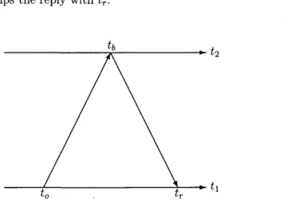
where U is the local clock in node i, a* and bi are its drift and offset parameters, and t is the real time. If node 1 wants to determine what are its relative drift and offset with respect to node 2 (ai2 and 612 respectively), an exchange of messages would take place in the following way (shown graphically in Figure 2.4):

1. Node 1 sends a message to node 2, which is timestamped right before it is sent

9X T/Q.

2. Node 2 timestamps the reception with fy,, and returns a reply to node 1 which includes £&.

3. Node 1 timestamps the reply with tr.

Figure 2.4: Exchange of messages to determine relative drift and offset between two nodes.

The three timestamps (t0,tb,tr) form a data-point which limits the values of

pa-rameters ai2 and bu- Since to —> tt, and £& —> tr, the following inequalities should

hold for the data points:

t0(t) < a12tb(t) + 612 ,

tr(t) > al2tb(t) + b12 .

After the acquisition of a few (at least two) data-points, an estimation of the parameters can be performed by solving the linear programming problem given by the inequalities formed by the data-points. As new data-points arrive, the number of data-points to keep can be reduced to only two by determining which ones result in the best estimates (tiny-sync method). Alternatively, up to 40 points can be used with a different way to eliminate old data-points (mini-sync method). The tiny-sync method results in a suboptimal solution.

To synchronize a multihop network, it is assumed that the sensor network is organized as a tree hierarchy with sensor nodes in the lowest layer, one (or more) root node(s), and possibly several layers of intermediate nodes. It is also assumed that data is fused at the intermediate nodes. So, instead of synchronizing the entire network to one unique clock, all nodes reporting to the same intermediate node should synchronize with such intermediate node using the exchange of messages described. Therefore, nodes in layer i synchronize with nodes in layer i — 1 and so on. The performance of the algorithm was tested on an 802.11b multihop ad hoc network, achieving an accuracy of 3 ms over a single hop.

2.5.5 Timing-sync protocol for sensor networks (TPSN)

In [16], a protocol, called TPSN, is proposed to achieve network-wide synchronization. In this protocol, the first step is to create a hierarchical topology in the network where

every node is assigned a level in the hierarchical structure. To create this hierarchical topology, the root (which is assigned level 0) initiates a level discovery phase when the network deploys, by broadcasting a level-discovery packet, which contains the identity and level of the sender. Once the neighboring nodes receive this packet, they assign themselves a level which is one greater than the level they have received and broadcast a new leveLdiscovery packet. This process continues until every node is assigned a level. Once a node has assigned itself a level, then further leveLdiscovery packets received are discarded.

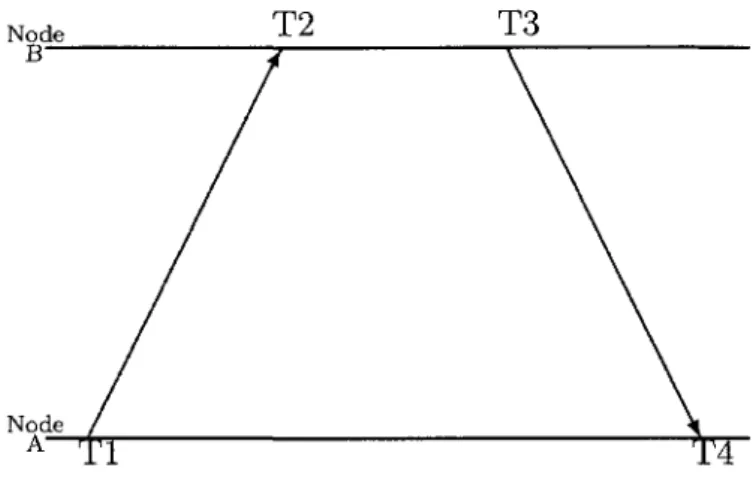
Once the level discovery phase ends, a synchronization phase starts where a node belonging to a level i synchronizes to level i-1. In this latter phase, a two-way message exchange occurs, and the clock drift and propagation delay are calculated, with the node making the calculations and correcting its clock accordingly. The two-way message exchange to synchronize two nodes A and B works in the following way (see Figure 2.5):

1. Node A sends a message (called synchronization pulse) to B at time T l . This message contains the level number of A and the value of T l .

2. Node B receives the message at time T2, where T2 = Tl + S + d, S and d being the clock drift between the two nodes, and the propagation delay, respectively. 3. Node B sends back an acknowledgment to node A at time T3, containing the

level number of B and the values of T l , T2 and T3. 4. Node A receives the acknowledgment at T4.

Node T 2 T3

B

Figure 2.5: Two-way message exchange, and propagation delay d as follows:

(T2 - T l ) - (T4 - T3) 5 =

(T2 - n ) + (T4 - T3)

This protocol was implemented on Berkeley MICA motes using a 4MHz crystal oscillator, after making modifications to the MAC layer so it could timestamp the messages at reception time. The accuracy obtained is around 17/xs for the synchro-nization of two motes.

2.5.6 Flooding time synchronization protocol (FTSP)

In [17], Flooding Time Synchronization Protocol (FTSP) is proposed to achieve clock synchronization on a wireless sensor network. It uses MAC layer timestamping ca-pabilities to eliminate several sources of error in the clock synchronization process: sending time, access time and receive time. In this protocol, it is assumed that a node, the root, which is elected after the exchange of messages in the network, is already

synchronized, and the other nodes synchronize with this node. The root broadcasts a message which includes the global time at the time of sending the message and root ID. The receiver gets a timestamp at the time of reception, and using the arrival and sending times, it estimates the clock offset and skew once a number of readings are available, using linear regression.

When a mote determines it is already synchronized, it also broadcasts packets which include the global time and root ID, creating in this fashion a clock synchro-nization hierarchy where the root is at Level 0, nodes within the broadcast range of the root at Level 1 and so on. Every node therefore estimates the global time by synchronizing its clock to the nodes one level higher than itself.

This protocol has been implemented in Berkeley MICA2 motes. The average accuracy obtained for a 60-node network is 16 fis.

2.5.7 Lightweight tree-based synchronization (LTS)

[18] proposes a tree-based synchronization method for sensor networks that requires the construction of a spanning tree in order to generate the pair-wise synchroniza-tions required to synchronize the whole network. It also proposes another method to synchronize a multihop network without requiring the construction of a tree, but assumes the use of a multi-channel MAC. Both versions were simulated but not im-plemented, and are aimed at minimizing the complexity of the synchronization and not in maximizing accuracy.

2.5.8 Adaptive clock synchronization

In [19], RBS is extended to provide an adaptive and probabilistic clock synchroniza-tion allowing a trade-off between the accuracy achieved and the resources used by the protocol. It has not been implemented.

2.5.9 Pairwise broadcast synchronization (PBS)

In [20], a new approach for clock synchronization is proposed. It uses the broadcast nature of the wireless channel, and allows a node to synchronize by overhearing syn-chronization packets exchanged in a similar fashion as TPSN among two neighboring nodes, without the need to send extra messages. This method reduces the number of messages required for synchronization but requires that all nodes hear each other. A multi-cluster extension has been proposed in [21], which requires the construction of a hierarchical tree and the use of groupwise pair selection algorithm to achieve global synchronization.

2.5.10 Gradient time synchronization protocol ( G T S P )

The Gradient Time Synchronization Protocol (GTSP) is proposed in [22]. The idea of this protocol is to provide a precise clock synchronization between neighboring nodes and allow a more loose synchronization between nodes separated by multiple hops. The algorithm does not require the construction of a hierarchical topology, or a reference node, but in order for it to converge, the network needs to be strongly connected. It has been implemented on a small network of 20 Berkeley MICA2 motes, obtaining an average error of 4 /is for direct neighbors, and a network-wide average error of 14 /xs.

2.5.11 Average time sync (ATS)

[23] proposes the Average Time Sync (ATS) to synchronize a multihop wireless sensor network. The protocol is formulated as a consensus problem, and achieves global clock synchronization to a virtual reference clock in a distributed manner. The protocol works by performing three tasks in each of the nodes: relative skew estimation, skew compensation and offset compensation. These tasks require only local information

exchanges between neighboring nodes, each of the nodes maintains its own estimate of the virtual reference clock, which is updated by averaging it with respect to the estimate that the neighboring nodes have. It has been implemented on Tmote Sky nodes [68].

As can be observed from the description of the protocols for clock synchronization in wireless sensor networks, with the exception of the last two ( [22,23]), either they rely on the construction of a hierarchical tree structure ( [15-18]), which generates a lot of overhead and does not support dynamic topology changes very well, or they rely on all the nodes sharing the media with a beaconing node ( [14,19,20] ), which makes them unsuitable for multihop networks.

The protocol described in Chapter 4 provides an efficient clock synchronization algorithm for wireless multihop networks without requiring the construction of a hierarchical structure. It is fully distributed and has been implemented on a Berkeley motes testbed with very good results.

C H A P T E R 3

BILATERAL CLOCK

SYNCHRONIZATION

A L G O R I T H M

This chapter presents the bilateral synchronization part of our new clock synchroniza-tion algorithm. The system model is described in Secsynchroniza-tion 3.1. The method to achieve a pair-wise synchronization between neighboring nodes is explained in Section 3.2.

3.1 System Model

It is assumed in this work that the clock drift in a node follows the linear equation: Ti = otit + Oi, just as in [11,15,17], where % is the local clock, oti and Oi are the drift parameters that express the relative speed of the clock and the offset respectively, and t is the real time. Nodes' clocks drift at different rates. Neighboring nodes exchange timestamps to estimate the best-fit offset line between them by using a recursive least squares (RLS) estimation approach. Further details are provided in Section 3.2.

Also assumed is the fact that all the nodes are aware of the set of neighbor nodes with which they can directly communicate, and that the communication links between the nodes are bidirectional.

3.2 Pair-wise Clock Synchronization between

Neighbors

In this section we very briefly describe how bilateral synchronization between two neighboring nodes is performed. This is not really novel, since it is just a variant of

linear regression.

Suppose we have two nodes i and j which can communicate directly, and want to determine their offset Oij and skew a^ by exchanging packets. By the offset Oij(t) we will mean the difference in the two clocks Tj(t) — Ti{t). By the skew a^ we will mean the ratio of the speeds —.

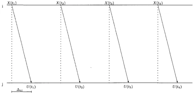
At time X(tk), node i sends a packet p(tk) that includes this timestamp, its latest estimate of its skew with respect to j , &ji(tk), and its latest estimate of the time difference between received and transmitted timestamps for packets from j to i, Tji(tk). Packet p(tk) is received at time U(tk) by node j . This is done frequently as can shown in Figure 3.1. With these packets, node j can compute the value <%(£&), which is the estimate of the skew of j with respect to % at real time tfc.

Figure 3.1: Frequent transmissions of estimates to neighbor node.

The value aij(tk) is estimated using Recursive Least Squares (RLS) [69] to solve the following problem:

fc-i

where A G (0,1) is the forgetting or weighting factor that reduces the influence of old data.

The RLS algorithm is widely used in adaptive filtering, system identification and adaptive control. It also allows us to estimate a with minimal storage requirements since only the previous and current values of U(t) and X(t) are required at any given time.

To develop the algorithm, we rewrite equation (3.1) as follows: fc-i

A

= m i n j ] A ^ - ' I T . - ^ A ]

,

T, = |£/fe

i)-tf(i,)|,

<pf = ixc^o-xct,)!,

We differentiate (3.2) with respect to A and set it to zero, i.e.,

dA k-l T A I2

J2 A*"

"' [T, - <f>fA]

and get the following:

fc-i

£

/=—oo

A k-l-l

r

- 4>fA

= o,

l=—oo

Let us define

fc-i

/=—oo

Then we can see that

Rk = XRk-i + 4>k4>k • Substituting (3.4) in (3.3) we get fc-i

R

-

A

= Y, A * -

" ' ^ , .

R

A

= £ A

-'0,T,

= 2 J A

' 0/T

+ 4>

T

Hence, multiplying by R^1, assumed to exist, we obtain

A

= (J - i£Vk^JO Afe + i£VkTfc

= A

+ R^V* (T

- <#A

) •

k - i

E

Z = — o o

fc-Now, we need to find a way to calculate Rk in a recursive fashion using only the information available at time k. For this, we use the Matrix Inversion Formula [69] that says the following:

If A and B are M x M invertible matrices, D is a N x N matrix, and C is a M x N matrix, which are related by

A = B~l + CD^CF ,

then

A"1 = B - BC (D + CTBC)_1 CTB,

whenever the inverses exist. We apply this formula to (3.5) using

D = 1, C = (f>k, B~ = XRk-i,

and

A = Rk,

and get the following

R^1 = (AJRfc_1)-1-(Ai?fc_x)-10fc(l + ^(AJRf c_1)-10f c)"1^(AJRf c_i)"1

Now, from (3.6) we see that we need to compute R^cfik, so Hk <pk -A -A (-A + < ^ ~ - -A )

R;y

(A + (fjR-^k) - R^MlRk-Jk

A + ^ K V * "

Therefore, we can now compute Afc+1 using values that are all known at time A;

with the following recursion:

s

*+> =

'

i ? S § * (

' - «

' )

Once the skew a.ij{tk) is computed, we can estimate the time at which the current

packet should be received, using a window of AT values of U(tk) and X(tk), by doing the following computation:

1 fc-i

U(tk) = jj E I

(*') + *«(**)(*(**)-*(*/))]. (3.7)

/=fc-JV

where

«i(tk) •= Jf^y (3-8)

Then, we can determine the difference between the received and transmitted times-tamps at nodes j and i, Ty. This is the sum of the offset of node j with respect to i, 0{j, and the transmission delay of the packet, Ay, at time tk. It is estimated by

subtracting X(tk) from U(tk):

However, we need to first determine the value of A^- so that we can estimate the value of Oij(tk). In order to achieve this, packets must be sent back from node j to node i and should include the following values: a^-, Tij(S) and the time S at which the packet was sent. Tij(S) is then computed as follows;

r

(5) = r

(t

) + (s-Ufa)) ^ - \ (3.10)

to account for the change in offset between Ufa) and S due to skew.

Node i executes the same procedure as node j . That is, it also estimates its skew with respect to j , dijifa), the time at which the packet should have been received, and its difference in time with respect to j , Tjifa).

Now, node i can estimate the value of the transmission delay as

A

fa) = r ^ + ^ f a ) ,

3.ii)

and then its offset with respect to j as

Ojifa) = r^fa) - Ajifa). (3.12)

Now, on the next packet, pfa+i), to be sent from node itoj, the values included

in it would be its most recently calculated skew, a^fa), its most recently calculated transmission delay, Ajifa), and the estimated offset at time tk+i, which is given by

63lfa+1) = O^fa) + (tk+1 - U(S)) a^t kl ~ \ (3.13)

This process is then repeated.

By this method we can obtain estimates of offsets and skews at given times be-tween two neighboring nodes.

3.3 Simulation Results

Before implementing the algorithm discussed, simulations were performed to verify if the behavior of the algorithm was as expected.

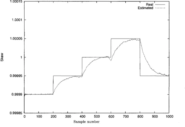
First, we simulated the pair-wise synchronization procedure with different values of A and N (forgetting factor for the RLS algorithm and window size to estimate U(i), respectively). We found through simulation with various values of A and N that values of A = 0.999 and N = 10 provide the best estimation accuracy without requiring too much memory space.

1.00015 5 CD 1.0001 1.00005 1 -0.99995 0.9999 f 0.99985 1 -r • i / i i y / t N 1 ,-""' i 1 1 Real Estimated /U' V " 'V> . -, \ \ \ \ 1 1 100 200 300 400 500 Sample number 600 700 800 900 1000

Figure 3.2: Skew estimation results obtained in simulation.

Then, the skew of one of the nodes simulated was modified frequently, within the ranges (±100ppm) of the physical oscillator [70] found on the experimental testbed to be used, during the course of the simulations in order to determine if the calculations of skew and offset adapt to the changes. We can see in Figure 3.2 that the skew

estimate indeed adapts to the real skew as it changes. Also, in Figure 3.3 we see that the difference between the real and estimated offsets between the two nodes is below

2 jis. 3= o a E 200 300 400 Sample number 500 800

Figure 3.3: Offset estimation results obtained in simulation.

3.4 Implementation on Berkeley Motes

For the implementation of the algorithm described in this chapter, as well as the one that will be presented in the next chapter, we used a testbed of MICA and MICA2 motes.

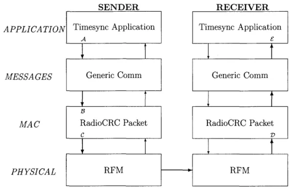
Figure 3.4, which shows the communication stack of TinyOS on the Berkeley motes, provides a better understanding of the sources of error in the clock synchro-nization process mentioned in Section 2.5.1 and how can we prevent some of them in TinyOS.

APPLICATION MESSAGES MAC PHYSICAL SENDER Timesync Application A ' ' Generic Comm 1 • B RadioCRC Packet c ' • DTT<l\/r RECEIVER Timesync Application £ i i Generic Comm • . i RadioCRC Packet V • L "DT7TVT x\r IVI

Figure 3.4: Communication stack on TinyOS 1.x.

• The message to be sent is constructed at the application layer and is then passed to the lower layers for its transmission. The time that it takes to construct the message and pass it down to the MAC layer is the send time. In Figure 3.4, it would be time period starting at the point the Clock Synchronization application calls sendMsg() (denoted by the symbol .4.), and ending at the reception of the message at the RadioCRCPacket component (denoted by the symbol B).

Once in the MAC layer, some time must elapse before the message is actually transmitted over the medium, since it has to wait until it has been determined that the medium is idle. This is the access time. In Figure 3.4, it would be the time period starting at the reception of the message at the RadioCRCPacket component (denoted by the symbol B), and ending at the time the first byte is sent for transmission to the Radio Module (denoted by the symbol C).

• Once the bits have been received at the receiver, the message is reconstructed and passed up to the application layer. The time taken to do all this is the receive time. In Figure 3.4 it would be time period starting at the reception of the first byte at the RadioCRCPacket component from the Radio Module (denoted by the symbol Z>), and ending at the time the message is received at the Clock Synchronization application (denoted by the symbol £).

Therefore, in order to reduce the sources of error in our implementation, we have modified the MAC layer of TinyOS to allow the timestamping of a packet at the time the first byte is sent, instead of doing it at the application layer. We also record the time at which the first byte is received by the MAC layer at the receiver side for later use by the application layer. In this way, we attempt to mitigate the send time, access time and receive time as sources of error, leaving only the propagation time, which is negligible in the case of the broadcast medium used in the Berkeley motes.

3.4.1 Setup

Sender Receiver

Figure 3.5: Implementation setup for two nodes.

sender and receiver as described before, and a third mote connected to a PC through the serial port acting as a data collector or gateway. This latter mote continuously senses the medium and communicates the data being transmitted to the PC. The sender and receiver exchange a clock synchronization message every 30 seconds. This setup is illustrated in Figure 3.5.

In order to get better accuracy, the motes' clocks were modified to generate a finer granularity clock, which is triggered by a crystal oscillator. The frequency of such crystals was modified in the MICA motes to 500 KHz. For this, the clock timer had to be changed since the original timer (Timer 0) uses an 8-bit register to maintain the clock counter. This would overflow at this frequency, and so we use instead Timer 1 which has a 16-bit clock counter. These changes were problematic since Timer 1 is already used for other purposes by TinyOS, and the conflicts raised had to be solved in order for TinyOS and our application to work correctly. For MICA2 motes, a component to use a higher frequency of 921.6 KHz was made available by Maroti et al. [71].

Although MICA motes were initially used for the implementation of the pair-wise synchronization, due to the lack of wireless reprogramming and support in newer versions of TinyOS, the subsequent experimentations were only performed on MICA2 motes.

3.5 Evaluation

In order to determine the accuracy of this protocol, the gateway mote periodically requests the time each mote has estimated. Both motes reply to this query, one with the time it has estimated at the other node, and the other node with its current time. The difference between the times replied is the accuracy or error of the protocol. By using this method to compare the times in both motes, we remove the send time,

zs c

O

150 200 250 300 350 Timestamp exchange number

500

Figure 3.6: Accuracy of estimated to real time between 2 neighboring nodes. access time, and propagation time as sources of error (see Figure 2.5.1).

With the implementation on MICA2 motes, we obtained an average accuracy of below 2//s (with a worst-case accuracy of 6/is) as can be seen on Figure 3.6. This is better than the accuracy obtained in the related works mentioned in Section 2.5, with the exception of [17]. It has similar results as ours since we use the same timestamping technique to eliminate most of the sources of error that appear when we try to synchronize nodes in a network through message exchanges [58].

Now that each node is able to estimate the time at each of its neighbors, we want all nodes to be able to agree on a common time. In the next chapter we address this problem.

C H A P T E R 4

M U L T I H O P CLOCK

SYNCHRONIZATION

We now turn to clock synchronization for a network of clocks. We address the problem of how to globally combine bilateral estimates of offset and skew into estimates of time with respect to the reference clock for each node in the network.

Just for simplicity of presentation, suppose that there are n nodes all having clocks running at exactly the same speed, except that they have different offsets. With node 1 chosen as the reference, let Zi denote the amount that node z's clock is ahead of node 1. So z\ = 0. Thus, if U(t) denotes the time at clock i at real time t, then

U(t) = t^t) + zt for all t. Let

be the offset between nodes i and j .

Let Ni denote the set of neighbors of node i, and |A^| the number of such neighbors. Assume that through experimentation as in Section 3.2, we have obtained esti-mates Xij of Xij = (zi — Zj) for j 6 Ni for all i. These estiesti-mates will not be exactly equal to the true values. We will also suppose that

Xji = —x^ for j G Ni for all i,

so that nodes i and j have talked to each other in arriving at this estimate (using the algorithm described in Chapter 3).

The problem is this: We want to obtain estimates Vi = 2i of the offsets with respect to the reference node.

4.1 Formulation

Note that the true x^-'s satisfy the global constraint

for every cycle

Z = ( ( « l , i 2 ) , ( « 2 , « 3 ) , - - - , ( * m , « l ) ) in the multihop network.

This is one example of a global constraint that needs to be satisfied by the offset between neighboring nodes. There are many such constraints because there are many cycles in the graph of the wireless network.

However, the estimates x^ arrived at through only bilateral transactions described in Chapter 3 need not satisfy these constraints.

By enforcing the large number of such constraints, the estimates {:%} can be smoothed and improved. We call this procedure "spatial smoothing." In essence, it exploits a spatial law of large numbers through a reformulation of the problem to lead to better clock synchronization with respect to any chosen reference node.

Moreover, we would like to perform such constrained estimation over the ad hoc network with the nodes acting in a completely distributed asynchronous manner. We will now develop an algorithm where each node only needs to asynchronously broadcast a few numbers. Each node updates its numbers through an extremely simple formula based on each received broadcast. This then will be shown to lead to

an estimate of the offset with respect to any node which acts as a reference node. Nodes will not need to know which is the reference node, or the topology of the network. No levels of hierarchies of nodes need to be constructed. In fact, our protocol exploits all edge offset estimates in the network, and not just those along a tree. In a large network it uses all the global information, and yet does so in a simple distributed asynchronous manner. Not all local broadcasts have to be received by any node either.

The manner of changing from one reference node to another, i.e., reference clock handoff, is also easy. The old reference node simply starts adapting, while the new one stops. The rest of the network automatically adapts to this change, and need not be explicitly informed of such reference handoffs.

We illustrate the method with a concrete example. For the network in Figure 4.1, there are five nodes { 1 , . . . , 5} and six arcs {(1, 2), (2,3), (3,4), (1,4), (2, 5), (3, 5)}.

Figure 4.1: Example of a network.

As a convention we shall take each arc as going from a lower lexicographically num-bered node to a higher one. Let A be the Node x Arc matrix, called the incidence

matrix: 1 2 3 4 5 (1,2) +1 -1 0 0 0 (2,3) 0 +1 -1 0 0 (3,4) 0 0 +1 -1 0 (1,4) +1 0 0 -1 0 (2,5) 0 + 1 0 0 -1 (3,5) 0 0 + 1 0 -1

where in the row corresponding to node i, we have an entry +1 for all arcs of the form (i, *), an entry —1 for all arcs of the form (*, i), and 0 otherwise.

Let Vi denote the estimate that we will make of Zi. Then the estimate of the offset between nodes i and j is Vi — Vj, which is the inner product, {(ij)-th. column of A, vector v). Hence, written as a vector of estimates of arc offsets, it is ATv.

Thus the problem formulation is:

Mmv\\ATv-x\\2. (4.1)

Note that this seeks the minimum norm approximation in the range space of AT to the vector x. The error of the approximation, by the Projection Theorem,

is orthogonal to R(AT), the range space of AT. That is, (ATv — x) is orthogonal to

R(AT). However R(AT)± = N(A), where N(A) is the null space of A. Thus (ATv-x)

is in the null space of A. Hence the solution of this optimization problem is

A(ATv-x) = 0,

or

Now let us consider the i-th row of A. It corresponds to node i. It has a ± 1 for every incident arc. Now the j'-th column of AT similarly has ± 1 for every arc incident to j .

Hence (AAT)a = # of neighbors of i = \Ni\. Also,

(AA^j = -ItijeNi

= O i f j ^ i V , .

Thus the i-th entry of AATv is

\Ni\Vi ~ Yl V

3-Also, the i-th. entry of Ax is the sum of terms of the form + 1 times £;*, or (—1) times x*i, which in either case is x^. Thus the i-th entry of Ax is

E

jeNi Xij.

Thus (4.2) can be written as:

\Ni\vi — 2_. vj = / J %ij f°r a u i- (4-3)

Note that this is deficient by at least one rank. So we set

vi := 0.

This corresponds to choosing node 1 as the reference node. We will now consider the problem:

We will solve the problem by coordinate descent since that will provide a fully distributed algorithm, in addition to being asynchronous. At the m-th iterate, let v(m) be the estimate. We can take the initial iterate as

v(0) := 0.

Also, since node 1 is the reference, we also have

i>i(m) := 0 for all m > 0.

We will minimize over Vi(k) perturbing it by Si to minimize the objective function (4.4), while keeping Vj(k) invariant for j ^ i. Now the only terms in which vi figures in (4.4) are V j€Ni jeNi J

I

\

i\

3 -^2

k~Yl

i

~

~

V

When we perturb Vi t o Vi + <5j, we get

[iNiKvi + SJ-^Vj + Xij)) +

\ jeNi )

X \Nj\V3 ~ Yl(Vk+ ^ -(vi + $i)- %ji ) jeNi

\

keNj k^i

Differentiating with respect to Si, and setting to 0 gives,

WllNiUvi + S^-^ivj+Xij)

— "Reported error of node j " .

({N^ + lNiDSi + lNilei-Y,^ = 0. jeNt Si = t-ujeN^J \^i\ei

IW + M

So the distributed algorithm is very simple: At each iterate, some node, say node i, changes its Vi to Vi + Si, where

Si := 1

\Nt\ + l

1

reE*

6

'-*)

jeNi

\Ni - [Average of (e,- — ej) reported by its neighbors j] i\ T 1

node can calculate:

ej = Wjlvj-^ivi + Xji).

It then adjusts its Vj to Vj + 5j. Then it rebroadcasts e_,-, etc. • Now, if the clocks do not run at the same speed, that is, they have a drift or

skew, a similar process would also have to be executed simultaneously to estimate the clocks' skews. If we substitute log(aji) for Xji we are able to use the same solution just discussed to estimate skews while taking global constraints into account.

Also, due to the difference in skews between the nodes' clocks, every time the error is computed by a node i for the offset estimation, the u,'s and Xjk's of all its neighboring nodes k should be adjusted using the latest estimation of their skew in a way similar to the one shown in equation 3.13.

One can also obtain an alternative algorithm for the problem of minimizing (4.1). If we take another look at the original problem formulation in (4.1), we see that since we are trying to minimize v, we can simply use the following recursion:

Vi = —-—-— J— for all i. (4.5)

Therefore we have another distributed algorithm which is even simpler. Each node j simply broadcasts to its neighbors (j,Vj) sporadically, and from this, each node i can calculate its Vi following (4.5).

A further modification is to only take the average in (4.5) with respect to nodes that are at a fewer number of hops in distance from the reference node.

In [72], Giridhar and Kumar have analyzed the least-squares approach used in this protocol by relating the optimization problem given by (4.1), to the problem of determining the electrical resistance between two nodes in an electrical network