Generic application of deep learning framework for real-time engineering data analysis.

AUTHOR(S):

TITLE:

YEAR:

Publisher citation:

OpenAIR citation:

Publisher copyright statement:

OpenAIR takedown statement:

This publication is made freely available under ________ open access.

This is the ___________________ version of proceedings originally published by _____________________________

and presented at ________________________________________________________________________________

(ISBN __________________; eISBN __________________; ISSN __________).

This publication is distributed under a CC ____________ license. ____________________________________________________

Section 6 of the “Repository policy for OpenAIR @ RGU” (available from

http://www.rgu.ac.uk/staff-and-current-students/library/library-policies/repository-policies

) provides guidance on the criteria under which RGU will

consider withdrawing material from OpenAIR. If you believe that this item is subject to any of these criteria, or for

any other reason should not be held on OpenAIR, then please contact

[email protected]

with the details of

the item and the nature of your complaint.

GREEN

MAJDANI, F., PETROVSKI, A. and PETROVSKI, S.

Generic application of deep learning framework for real-time engineering data analysis.

2018

MAJDANI, F., PETROVSKI, A. and PETROVSKI, S. 2018. Generic application of deep learning framework for real-time engineering data analysis. In Proceedings of the International joint conference on neural networks 2018 (IJCNN 2018), 8-13 July 2018, Rio de Janeiro, Brazil. Piscataway: IEEE [online], article ID 8489356. Available from: https://doi.org/10.1109/IJCNN.2018.8489346

MAJDANI, F., PETROVSKI, A. and PETROVSKI, S. 2018. Generic application of deep learning framework for real-time engineering data analysis. In Proceedings of the International joint conference on neural networks 2018 (IJCNN 2018), 8-13 July 2018, Rio de Janeiro, Brazil. Piscataway: IEEE [online], article ID 8489356. Held on OpenAIR [online]. Available from: https://openair.rgu.ac.uk

AUTHOR ACCEPTED

International joint conference on neural networks 2018 (IJCNN 2018), 8-13 July 2018, Rio de Janeiro, Brazil 9781509060146 2161-4393

© 2018 IEEE. Personal use of this material is permitted. Permission from IEEE must be obtained for all other uses, in any current or future media, including reprinting/republishing this material for advertising or promotional purposes, creating new collective works, for resale or redistribution to servers or lists, or reuse of any copyrighted component of this work in other works.

BY-NC 4.0 https://creativecommons.org/licenses/by-nc/4.0

https://mirrors.creativecommons.org/presskit/buttons/88x31/png/by-nc.png[10/10/2017 09:37:50]

OpenAIR at RGUDigitally signed by OpenAIR at RGU

Generic Application of Deep Learning Framework

for Real-Time Engineering Data Analysis

Farzan Majdani

and Digital Media, Aberdeen, UK,

Email: [email protected]

Andrei Petrovski

and Digital Media, Aberdeen, UK, Email: [email protected]

Sergei Petrovski

Samara State Technical University, School of Electric Substations,

Samara, Russian Federation, Email: [email protected]

Abstract—The need for computer-assisted real-time anomaly detection in engineering data used for condition monitoring is apparent in various applications, including the oil and gas, automotive industries and many other engineering domains. To reduce the reliance on domain-specific experts’ knowledge, this paper proposes a deep learning framework that can assist in building a versatile anomaly detection tool needed for effective condition monitoring.

The framework enables building a computational anomaly detection model using different types of neural networks and supervised learning. While building such a model, three types of ANN units were compared: a recurrent neural network, a long short-term memory network, and a gated recurrent unit. Each of these units has been evaluated on two benchmark public datasets. The experimental results of this comparative study revealed that the LSTM network unit that uses the sigmoid activation function, the Mean Absolute Error as the objective Loss function and the Adam optimizer as the output layer showed the best performance and attained the accuracy of over 77 % in detecting anomalous values in the datasets.

Having determined the best performing combination of the neural network components, a computational anomaly detection model was built within the framework, which was successfully evaluated on real-life engineering datasets comprising the time-series datasets from an offshore installation in North Sea and another dataset from the automotive industry, which enabled exploring the anomaly classification capability of the proposed framework.

Index Terms—Long short-term memory networks, deep learn-ing framework, anomaly detection and classification, time series analysis, engineering applications.

I. INTRODUCTION

Condition monitoring in general, and anomaly detection in particular, is an essential component of many safety and surveillance systems, because such monitoring is capable of uncovering informative facts about the behaviour, character-istics and properties of engineering systems used in various technical and technological areas. The main purpose of con-dition monitoring is undoubtedly to prevent the escalation of undesirable effects on system operation and to minimize losses caused by them [9]. This is critically important in various engineering systems the authors worked with, such as automobile engines, offshore installations, subsea hydraulic control, and autonomous surveillance [23].

These complex systems share at least two characteristics: a lack of mathematical model that accurately describes the system behaviour and a large amount of monitoring data that can be both historical and real-time. Therefore, for performing effective anomaly detection, it is necessary to rely on data-based approaches and on smart methods of condition moni-toring that often use computational intelligence and machine learning techniques [15]. The latter is especially important when some constraints are present that cannot be satisfied by human intervention with regard to decision making speed in life threatening situations (e.g. automatic collision systems, exploring hazardous environments,processing large volumes of data). Because computer-assisted condition monitoring is capable of processing large amounts of heterogeneous data much faster and is not subject to the same level of fatigue as humans, its use in many practical situations is preferable. Furthermore, the integration of multiple data sources into a unified system leads to data heterogeneity, often resulting into difficulty, or even infeasibility, of human processing, especially in real-time environments.

Computational Intelligence (CI) and Machine Learning (ML) techniques have been successfully applied to problems involving the automation of anomaly detection in the process of condition monitoring [15], [17]. In particular, many studies have shown that artificial neural networks (ANN) can be a very effective classification tool to predict various anomalous conditions, such as the corrosion of oil and gas pipelines, turbine failure, and the like [8], [21], [25].

However, one of the most significant factors to consider when performing engineering data analysis is a possible in-terdependence of sensors’ readings. It is important therefore to firstly identify the most significant features, or hyper-parameters, in the dataset and to take temporal dependencies of sensory data into consideration. A Long Short-Term Memory (LSTM) network is a type of recurrent neural network (RNN), specifically designed for sequence processing. It excelled in many complex challenges such as handwriting recognition [12], machine translation [26], and financial market prediction [10]. LSTM networks contain gates to store and read out information from linear units, called error carousels, that retain information over long time intervals - something that

traditional RNNs fail to achieve. In recognition of speech and hand writing, anomalies correspond to situations where the order of words or symbols is incorrect; similar, in engineering data analysis, the order and occurrence of certain data values can identify unusual patterns that ultimately may lead to a system failure.

Anomaly detection is an important data analysis task that detects anomalous or abnormal data from a given dataset. It has been widely studied in statistics and machine learning, and generally defined as ”an observation which deviates so much from other observations as to arouse suspicions that it was generated by a different mechanism” [1]. Anomalies are considered important because they indicate significant but rare events and can prompt critical actions to be taken in a wide range of application domains (for instance when the generator’s rotor speed of a gas turbine goes below 3000 rpm). By their nature, these events are rare and often not known in advance - this makes it difficult for conventional machine learning techniques, based on a generic ANN for instance, to be trained and optimised in terms of performance [9]. A wide variety of studies has been carried out to identify an optimised ANN model by altering weights, number of hidden layers, fine tuning hyper-parameters and altering activation functions [2], [16], [27], [28].

Although all these studies provide a good and effective approach in developing an accurate ANN model, they still require human intervention to optimise its performance by fine-tuning the ANN parameters mentioned above. Engineer-ing data analysis in industries, such as oil and gas for example, would often benefit from restricting, or even, eliminating human intervention in detecting anomalies. Thus, this paper proposes an approach to designing machine learning algo-rithms that can automatically select required hyper-parameters by using a generic LTSM network with a fixed activation layer capable of detecting an anomaly or predicting system failure. To the best of our knowledge, this study is the first to evaluate a deep learning framework for real-time engineering data analysis that fits an LSTM network into the process of identification and classification of anomalous data. The rest of the paper is organized as follows: Section II describes the methodology of building a generic framework for anomaly detection based on systematic data processing. Then two case studies will be discussed that demonstrate the capabilities of the proposed framework in detecting and classifying data anomalies. The evaluation of the exemplified framework on the datasets corresponding to the case studies is presented in Section III, while Section IV draws conclusions and speculates possible future work.

II. METHODOLOGY

In time series data anomalies can be categorized into: outliers, unusual data points significantly dissimilar to the remaining points in the data set, and anomaly patterns, which group fractions of data together, which are different from the majority of normal data. To deal with these categories, var-ious anomaly detection algorithms have been developed that

are classified into five major groups: probabilistic, distance-based, reconstruction-distance-based, domain-distance-based, and information-theoretic-based [15]. Different types of algorithms are more applicable in various scenarios of data analysis, which brings to front the idea of a generic framework capable of combining several analytic tools and approaches.

The idea of developing a framework of tools for anomaly detection is not new - in particular, in [1] the authors proposed a generic framework for network anomaly detection, focusing on analyzing network traffic. We adopt a similar approach, but with a prime interest in analyzing real-time engineering data coming from condition monitoring sensors.

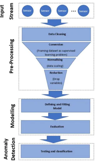
The proposed approach to developing an anomaly detection framework segregates processing of the input data streams ac-quired by physical sensors into three distinct phases. The Pre-processing phase is when the data gets prepared to be passed onto the anomaly detection algorithm by going through four different stages of data cleaning, conversion, normalization and reduction. The Modelling phase involves running a machine learning algorithm on training data that results in defining, fitting and evaluating a computational model, which will be used later on to identify anomalous data. In the final Anomaly Detection phase a new dataset gets tested with the purpose of determining the accuracy of the developed model. Figure 1 illustrates this anomaly detection process and the following subsections describe the stages of each phase.

A. Data Pre-Processing Phase

As was mentioned above, the Pre-processing phase consists of four different stages: data cleaning, conversion, normal-ization and reduction. During the data cleaning stage all invalid and inaccurate sensor values are removed, and all the qualitative values (i.e. texts and descriptions) are replaced with an index number corresponding to each word in the vocabularies used.

In general, time series data analysis can be viewed as a supervised learning problem. The advantage of this view is that re-framing time series data into supervised data frames enables using both standard linear and nonlinear machine learning algorithms. Therefore, at this stage of data pre-processing, all time series variables get merged together and are converted into supervised data frames through the approach adapted from [3]. In order to be able to use the majority of activation functions, including sigmoid, and also being able to plot the acquired data, all data values are scaled down to the range between 0 and 1 using a re-scaling function (see Algorithm 1. Algorithm 1 summarizes the data cleaning process applied to the pre-processed dataset and includes scaling and normal-ization of the data so that it can be passed onto the next phase. The final stage of data reduction is potentially one of the most important steps of data pre-processing aimed at avoiding over-fitting the analytic model that is going to be built. Through data reduction we can eliminate all redundant and non-informative features in the dataset, which will have a direct impact on the evaluation accuracy of the model to be developed.

Algorithm 1 Data Processing

1: dataProcessing (dataset)

2: unitToDrop←25%

3: Parse dates to format

4: repeat

5: /*Parse dates to format*/

6: fori←1, rowsdo

7: covert text or milliseconds to datetime

8: Covert qualitative values into quantitative ready

9: for LSTM

10: Frame multivariate time series as a

11: supervised learning dataset using lag time step (t-1)

12: Drop missing fields

13: Scale and transform

14: end for

15: untildata is scaled and normalized

16: Split Training and Test based on UnitToDrop

17: repeat

18: Reshape Training Dataset

19: fori←1, rowsdo

20: Reshape Training dataset to 3 Dimension

21: Reshape Test dataset to 3 Dimension

22: end for

23: untiltraining and test datasets are reshaped

24: Return (trainingDataset, testDataset)

B. Data Modelling Phase

Some of the widely used Recurrent Neural Networks (RNN) include Gated Recurrent Units (GRU), Hyperbolic Tangent (tanh) units and Long Short-Term Memory units (LSTM). However, the GRU and LSTM units proved to be more superior to conventional tanh units [7]. Therefore, in this study we are evaluating two closely related variants of the LSTM and GRU units on two publicly available datasets of Beijing PM2.5 [18] and Appliances Energy Prediction [19]. The PM2.5 dataset represents tiny particles or droplets in the air related to the quantity of air pollutant that is a concern for people’s health when its level is high. The dataset has being recorded on an hourly basis from US Embassy in Beijing, gathered over a 4-year period between 2010 and 2014. The other dataset consists of temperature and humidity sensor readings around a house, sampled every 10 minutes for about 4.5 months using a ZigBee wireless sensor network.

Three different data modelling approaches of using a simple RNN unit, a GRU unit and an LSTM unit on both datasets have been tested to determine which RNN unit outperforms the others (see Table I).

As can be seen from Table I, the LSTM unit demonstrated the best performance in terms of attaining the least validation loss .Loss is a summation of the errors made for each iteration of optimization on the training dataset batch.This value for test dataset batch is referred to as Validation Loss. Other studies also corroborate our finding that the LSTM approach applied for data analysis tasks involving long time lags performs better

Fig. 1. Systematic Approach to Context Processing

than other RNN units [11].

The computational model developed using LSTM has been tested and evaluated against such optimizers as Stochastic Gradient Descent (SGD), Adam, Adamax and Nesterov-Adam (Nadam). Amongst all those, the Adam optimiser outper-formed the rest (see Table II).

Another important factor to consider while tuning the model was the selection of an activation unit. Various activation units, including softmax, exponential linear unit (ELU), scaled exponential linear Unit (SELU), hyperbolic tangent (tanh) and sigmoid, have been tested. The sigmoid unit generated the best result and has been selected as the ultimate activation. Table

TABLE I ALGORITHM COMPARISON Dataset LSTM GRU RNN Loss Val. Loss Loss Val. Loss Loss Val. Loss Beijing PM2.5 1.78% 1.70% 1.86% 1.76% 1.98% 1.89% Appliances energy prediction 2.65% 4.18% 2.69% 4.20% 2.72% 4.21%

III lists the best recorded performance for all activation unit evaluated in this study.

Moreover, several objective (loss) functions have been eval-uated to find the optimal one for each dataset. These include the Mean Squared Logarithmic Error (MSLE), Mean Squared Error(MSE), Mean Absolute Error (MAE), Sparse Categorical Crossentropy (SCC) and Cosine proximity (CP). As it is shown in Table IV, the MAE function is the best in maintaining both accuracy and validation accuracy inline whilst generating the best result in terms of the smallest loss rate. In our further discussions we will use the following performance measures: (a) the Loss, which is the percentage of incorrectly classified data points; (b) the Value Loss that indicates the percentage of loss whilst training; (c) the Accuracy is the percentage of accurately classified data points in the training dataset; and (d) Accuracy Validation is the accuracy of the model on test datasets.

For developing the proposed framework a wrapper library Keras was used built around well-known python Neural Net-work libraries such as Theano and Tensorflow. With the help of all these libraries, a computation model for detecting anomalies in in the datasets was developed. As it is shown in Algorithm 2, the LSTM unit and Output layer with sigmoid activation are added to the model. The model is then compiled with the MAE loss function and the Adam optimiser, because these led to the best performance shown in Tables III and IV. The model is built by going through 50 training iterations (see table V). Also, for the demonstration and knowledge sharing

TABLE II

OPTIMISERCOMPARISON

Optimisers Loss Val. Loss

SGD 5.92 5.95% Adam 1.70% 1.70& Adamax 1.85 1.75 Nadam 1.78 1.75 TABLE III ACTIVATIONCOMPARISON

Activations Loss Val. Loss sigmoid 1.70% 1.70& softmax 1.76% 2.34& ELU 1.48% 2.42& SELU 1.46 2.30 tanh 1.85 2.08 TABLE IV

LOSSFUNCTIONCOMPARISON

Loss Functions Loss Val. Loss MSE 1.70% 1.70& MAE 1.73% 1.75& MSLE 2.32% 2.24&

SCC 1.8 5.4

CP 9.35 12.02

purposes the Jupyter Notebook interactive computational en-vironment has been utilized.

TABLE V

MODELPARAMETERS

Parameter Values

Optimiser Adam

Loss Function Mean Absolute Error (MAE) Activation Sigmoid

Iterations 50

Algorithm 2 Master Algorithm

1: TrainAndValidate (trainingData, testData)

2: model←sequential() 3: cell←0 4: activation←sigmoid 5: loss←mae 6: optimizer←Adam 7: epochs←100

8: Get input shape from trainingData

9: Get number size of cell recurrent state

10: Create new LSTM unit

11: Assign cell and input shape

12: Add LSTM unit to model

13: Create new Dense Layer

14: Add Dense layer to model

15: Set activation for Dense layer

16: Compile model using Optimiser and Loss

17: repeat

18: /*Fit Model*/

19: fori←1, epochsdo 20: Evaluate Loss

21: Evaluate Validation Loss

22: Evaluate Accuracy

23: Evaluate Validation Accuracy

24: end for

25: until All epochs completed

26: Return (Loss, ValLoss, Acc, ValAcc)

It has been shown that a variant of the LSTM approach -the stacked LSTM (SLSTM) network is able to learn higher level temporal patterns without prior knowledge, and thus can potentially outperform a single layer LSTM network [20]. Another alternative is to use Bidirectional LSTM (BLSTM) networks, which can improve performance of the initial model based on a single layer LSTM network [11]. Although the initial model that operates with the sigmoid activation unit, the MAE loss function and the Adam optimiser has been proven to be effective and well performing, we have extended our study further by also evaluating the BRNN and SLSTM variants of RNN networks (see Table VI).

The comparative results of these evaluations demonstrate that neither of those approaches can outperform a single layer LSTM network. Instead, they introduce additional overheads to the training process, which slow it down, and increase

memory requirement. Although the BRNN network can poten-tially improve the performance on some occasions, our study revealed no significant benefit of using the BRNN alternative to the initially proposed one.

C. Anomaly Detection Phase

Having established the best performing composition of the computational model that is going to be used for real-time engineering data analysis, we were in the position to evaluate the developed framework on three different datasets. These datasets are described in the following subsections.

1) Identification of Anomalies: Compressor and Turbine datasets: It is a common practice that most of the sensory data acquired when monitoring the condition of an oil and gas offshore platform are stored in a data historian system, such as the PI system, which acts as a repository to store engineering data gathered from one or multiple installation. In this study we used the historical sensor data obtained from a gas turbine and from a high pressure oil-flooded screw compressor that operated on an offshore installation in the North Sea. This data is transmitted onshore in in real-time via a satellite Internet link.

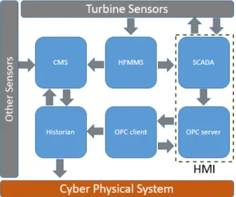
Most of the turbine’s sensory data goes straight to the connected High Frequency Machine Monitoring System (HFMMS) as illustrated in Figure 2. This happens due to the high volume of data generated every fraction of a seconds, which makes it almost impossible for any other system to handle such a volume. These sensor values are then passed onto a Conditional Monitoring System (CMS) to carry out the actual monitoring aimed at preventing failures of the turbine. The CMS uses a variety of measures and thresholds for assuring safety conditions and efficiency of the turbine. The sensory data that is not essential for the operation of CMS, but needed for controlling different units of the turbine, is passed straight into the human machine interface (HMI) system running the SCADA and OPC (OLE for Process Control) Server software. The HMI system can read all sensor values from both turbine and compressor, as well as being able to send some feedback signals to certain activators for control purposes. The OPC Server writes data to an OPC Client, which in turn store the data on the historian.

We used the anomaly detection model described in the previous section to identify anomalous values in the voltage output of the gas turbine using data from 32 input sensors acquired over a four-month period. The second data set used in

TABLE VI

UNIT COMPARISON

Dataset Basic LSTM Bidirectional Stacked LSTM Loss Val. Loss Loss Val. Loss Loss Val. Loss Beijing PM2.5 1.78% 1.70% 1.77% 1.69% 1.84% 1.77% Appliances energy prediction 2.65% 4.18% 2.68% 4.27% 2.69% 4.55%

Fig. 2. Data Monitoring Flow

this study represents a case when abnormal levels of compres-sor discharge pressure need to be found using the data gathered from 26 sensors over a two-week period. The developed framework tries to identify anomalies in these datasets through prediction of expected trends in output voltage trend for the gas turbine (using a 15-day interval) and in discharge pressure for the compressor (using a 7-day interval). The length of the prediction interval is determined by the size of the dataset used.

2) Classification of Anomalies: Interference Dataset: The next dataset records the effect of an interference-suppression capacitor in terms of noise reduction at different frequencies when no capacitor is present, and when the capacitor is connected to the bonding or to the engine cylinders [23]. Anomalies in interference voltage can be detected in any of the three options of connecting the interference-suppression capacitor when the noise level is changing too abruptly (Figure 3). The same anomaly detection computational model based on the LSTM network built earlier is applied to this experimental dataset.

In Figure 3, the small, medium and large diapasons of frequency values are 10, 20 and 50 MHz respectively - these are shown by the moving averages (MA) curves; the blue (main) curve represent experimental data related to interfer-ence voltage at different frequencies. Instead of using a single value, the intervals of 1.25, 2.5 and 7.5 dBV are used to compare between the actual and the modelled values. If the differences are larger or smaller than the specified limits in at least two of the three ranges of frequencies, then the value is considered anomalous.

Figure 3 is derived using the data on the interference voltage (y-axis) for frequencies above 65 MHz when interference-suppression capacitor connected to the engine is used. As shown, the anomalous frequency diapasons (x-axis) are 53-56, 133-150 and 177-180; this equates to the frequency ranges of 86.97-87.30, 96.25-98.34 and 101.76-102.15 MHz. As can be

Fig. 3. Possible anomalous interference

seen from Figure 3, five potential anomalies are identified. The result coincides with the expert knowledge obtained and can be attributed to excessive noise.

III. EXPERIMENTALRESULTS

For each dataset described above different prediction period has been tested depending on the number of items in the dataset. One of the challenges faced during the framework testing stage was data overfitting. In the scenarios when the training dataset was over 80 percent of the total available records in the dataset, an increasing accuracy of the model was observed with each training iteration, whereas the validation accuracy was gradually dropping. By keeping the training and test proportion at around the 80:20 level, we could success-fully predict future values, and as a consequence anomalous readings, for all the datasets used in this study. In Figures 4 - 9 the x-axis represent the total number of iteration and the y-axis represent either accuracy or loss percentages.

After going through the pre-processing phase to prepare the data for building anomaly detection models, we could train and test the models with exceptionally high accuracy and with minimal effort. For the compressor dataset , the loss and validation loss characteristics of nearly 0.01 were obtained, as it is illustrated in Figure 4.

The same characteristics for the turbine dataset were even closer to zero, being only 0.001 (see Figure 5).

Since the compressor dataset was smaller (covering the sampling period of 2 weeks), we could successfully predict the system operation for the next 7 days with the accuracy of 100 percent (see Figure 6).

On the other hand, for the turbine dataset covering the period of over 4 months, the prediction of its operation in the following 15 weeks was obtained with the validation accuracy of 77.6 percent. Although the model accuracy was higher (around 87 percent), in order to avoid data overfitting the

Fig. 4. Compressor Loss

Fig. 5. Turbine Loss

anomaly detection model could not be improved any further (see Figure 7).

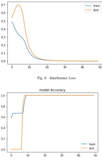
To evaluate the framework further and to test the classifi-cation capability of the designed anomaly detection model in classifying non time-series datasets, the electromagnetic inter-ference dataset was used. In addition to detecting anomalies in this case study, the task was to segregate them into three classes corresponding to difference values of the interference-suppression capacitance used. The Interference dataset was not in the form of a time series, so during the conversion stage of the data pprocessing phase the datasets was re-framed to enable the use of the same anomaly detection model. After training the model and testing it against the interference voltage dataset, the resultant loss and validation loss of 0.0003 were obtained (see Figure 8); also, the accuracy characteristics for the dataset attained 100 percent, as shown in Figure 9.

IV. CONCLUSION

In this paper a generic framework has been proposed aimed at detecting anomalies in real-time engineering data acquired in the process of condition monitoring. The framework enables the utilization of various deep learning techniques in building a generic anomaly detection model capable of not only identify-ing the presence of anomalous values in the analyzed datasets,

Fig. 6. Compressor Accuracy

Fig. 7. Turbine Accuracy

but of classifying these values for more effective condition monitoring.

When building such a model, three types of recurrent neural network units were compared: a recurrent neural network (RNN), a long short-term memory (LSTM) network, and a gated recurrent unit (GRU). Each of these units has been evaluated on two benchmark public datasets (Beijin’s air pollu-tion and Appliances energy predicpollu-tion datasets) in combinapollu-tion with various objective functions, with different Output layers (referred to as optimizers) that utilize a set of activation functions. The experimental results of this comparative study revealed that the LSTM network unit that uses the sigmoid activation function, the Mean Absolute Error as the objective Loss function and the Adam optimizer showed the best per-formance and results in a high model accuracy of over 77 % for the datasets it has been tested on.

Having determined the best performing combination of the neural network components, a computational anomaly detection model was built within the framework, which was evaluated on real-life engineering datasets comprising the time-series datasets from an offshore installation in North Sea and another dataset from the automotive industry, which enabled exploring the anomaly classification capability of the

Fig. 8. Interference Loss

Fig. 9. Interference Accuracy

proposed framework.

One possible direction of future research is to adapt the framework for detecting anomalies in much larger datasets coming from other application domains and acquired by using modern instrumentation technologies, including Internet of Things and wireless sensor networks.

ACKNOWLEDGMENT

The authors would like to thanks our industrial collabora-tors (who requested their identity to remain confidential) for providing the required datasets and for their general support. The authors would also like to thanks the developers of Theano, Tensorflow, Keras and Jupyter software extensively used throughout this work.

REFERENCES

[1] Ahmed, M., Mahmood, A. N., and Hu, J, 2016. A survey of network anomaly detection techniques. Journal of Network and Computer Appli-cations, 60, pp. 19-31.

[2] Beiko RG, Charlebois RL (2005) GANN: genetic algorithm neural networks for the detection of conserved combinations of features in DNA. BMC Bioinformatics 6:36

[3] Brownlee, J., 2017. Introduction to Time Series Forecasting With Python. URL: https://machinelearningmastery.com/introduction-to-time-series-forecasting-with-python/

[4] Che, Z., Purushotham, S., Cho, K., Sontag, D. and Liu, Y., 2016. Recurrent neural networks for multivariate time series with missing values. arXiv preprint arXiv:1606.01865.

[5] Chen, M., Mao, S. and Liu, Y., 2014. Big data: A survey. Mobile Networks and Applications, 19(2), pp.171-209.

[6] Cortes, C. and Vapnik, V., 1995. Support-vector networks. Machine learning, 20(3), pp.273-297.

[7] Chung, J., Gulcehre, C., Cho, K. and Bengio, Y., 2014. Empirical evaluation of gated recurrent neural networks on sequence modeling. arXiv preprint arXiv:1412.3555.

[8] El-Abbasy, M.S. et al., Artificial neural network models for predicting condition of offshore oil and gas pipelines. Automation in Construction, 45, pp. 50-65 (2014)

[9] Fanaee-T, H., Gama, J., 2016. Tensor-based anomaly detection: An interdisciplinary survey. Knowledge-based Systems, 98, pp.130-47. [10] Fischer, T., Krauss, C., 2018. Deep learning with long short-term

memory networks for financial market prediction. European Journal of Operational Research, in press, pp.1-16.

[11] Gers, F.A., Schraudolph, N.N. and Schmidhuber, J., 2002. Learning precise timing with LSTM recurrent networks. Journal of machine learning research, 3(Aug), pp.115-143.

[12] Graves, A., Liwicki, M., Fernndez, S., Bertolami, R., Bunke, H. and Schmidhuber, J., 2009. A novel connectionist system for unconstrained handwriting recognition. IEEE transactions on pattern analysis and ma-chine intelligence, 31(5), pp.855-868.

[13] Hansen, L.K. and Salamon, P., 1990. Neural network ensembles. IEEE transactions on pattern analysis and machine intelligence, 12(10), pp.993-1001.

[14] Hecht-Nielsen, R., 1988. Theory of the backpropagation neural network. Neural Networks, 1(Supplement-1), pp.445-448.

[15] Kanarachos, S., Christopoulos, S.-R., Chroneos, A., and Fitzpatrick, M., 2017. Detecting Anomalies in time series data via a deep learning algorithm combining wavelets, neural networks and Hilbert transfroms. Expert Systems with Applications, 85, pp.292-304.

[16] Karzynski M, Mateos A , Herrero J, Dopazo J (2003) Using a genetic algorithm and a perceptron for feature selection and supervised class learning in DNA microarray data. Artif Intell Rev 20(12):3951

[17] Khan, Z., Shawkat Ali, A. B. M., and Rhttps://www.sharelatex.com/project/5860d5a64fa3ca7871c258f9iaz, Z., Eds., Computational Intelligence for Decision Support in Cyber-Physical Systems. Springer, (2014)

[18] Liang, X., Zou, T., Guo, B., Li, S., Zhang, H., Zhang, S., Huang, H. and Chen, S. X. (2015). Assessing Beijing’s PM2.5 pollution: severity, weather impact, APEC and winter heating. Proceedings of the Royal Society A, 471, 20150257.

[19] Luis M. Candanedo, Veronique Feldheim, Dominique Deramaix, Data driven prediction models of energy use of appliances in a low-energy house, Energy and Buildings, Volume 140, 1 April 2017, Pages 81-97, ISSN 0378-7788

[20] Malhotra, P., Vig, L., Shroff, G. and Agarwal, P., 2015. Long short term memory networks for anomaly detection in time series. In Proceedings (p. 89). Presses universitaires de Louvain.

[21] Majdani, F., Petrovski, A. and Doolan, D., 2017. Evolving ANN-based sensors for a context-aware cyber physical system of an offshore gas turbine. Evolving Systems, pp.1-15.

[22] McCulloch, W.S. and Pitts, W., 1943. A logical calculus of the ideas immanent in nervous activity. The bulletin of mathematical biophysics, 5(4), pp.115-133.

[23] Rattadilok, P., Petrovski, A., and Petrovski, S., 2013. Anomaly Moni-toring Framework Based on Intelligent Data Analysis. In the Proceedings of the 14th International Conference on Intelligent Data Engineering and Automated Learning (IDEAL 2013), October 2013, Hefei, China. Springer Global, Lecture Notes in Computer Science, volume 8206, pp. 134-141. DOI: 10.1007/978-3-642-41278-3-17.

[24] Sak, H., Senior, A. and Beaufays, F., 2014. Long short-term memory based recurrent neural network architectures for large vocabulary speech recognition. arXiv preprint arXiv:1402.1128.

[25] Schlechtingen, M. and Santos, I.F., Comparative analysis of neural network and regression based condition monitoring approaches for wind tur-bine fault detection. Mechanical systems and signal processing, 25(5), pp. 1849-1875 (2011)

[26] Sutskever, I., Vinyals, O. and Le, Q.V., 2014. Sequence to sequence learning with neural networks. In Advances in neural information process-ing systems (pp. 3104-3112). Vancouver

[27] Taheri M, Mohebbi A (2008) Design of artificial neural networks using a genetic algorithm to predict collection efficiency in venturi scrubbers. J Hazard Mater 157(1):122129

[28] Tong, D.L. and Mintram, R., 2010. Genetic Algorithm-Neural Network (GANN): a study of neural network activation functions and depth of genetic algorithm search applied to feature selection. International Journal of Machine Learning and Cybernetics, 1(1-4), pp.75-87.