Ana Sofia Fachada Fernandes
P
ROGNOSTIC
M
ODELLING OF
B
REAST
C
ANCER
P
ATIENTS
–
A
B
ENCHMARK OF PREDICTIVE MODELS WITH
EXTERNAL VALIDATION
Dissertação apresentada para obtenção do Grau de Doutor em Engenharia Electrotécnica e de
Computadores – Sistemas Digitais e Percepcionais pela Universidade Nova de Lisboa, Faculdade de Ciências e Tecnologia.
LISBOA
Sumário
Existem inúmeros modelos de prognóstico clínico na área médico e particularmente no prognóstico do cancro da mama. Previamente à sua utilização clínica, os modelos de prognóstico necessitam de ser aplicados a pacientes provenientes de diferentes centros médicos, de forma a que sejam submetidos a uma rigorosa validação. Esta tese avalia a precisão preditiva de um modelo flexível com uma regularização Bayseana, o PLANN-ARD. Para tal utiliza uma base de dados composta por 4016 registos de pacientes com cancro da mama, diagnosticados de 1989 a 1993 e identificados pelo BCCA, Canada, com um follow-up
de 10 anos. Este método é comparado com a regressão de Cox, sendo considerado o modelo mais utilizado neste género de análise.
Ambos os métodos foram ajustados a 931 pacientes cujos dados de rotina foram adquiridos e diagnosticados entre 1990 e 1994 no Christie Hospital, UK, com um follow-up de 5 anos. Nesta tese foram desenvolvidos avanços metodológicos significativos que suportam a validação externa desta rede neuronal com dados clínicos, nomeadamente: imputação dos dados em falta em ambas as bases de dados, treino e validação e um índice de prognóstico que permite a estratificação dos pacientes em grupos de risco diferentes. A precisão preditiva dos modelos foi medida empiricamente utilizando o índice de descriminação standard, Ctd e uma medida de calibração utilizando o teste estatístico, Hosmer-Lemeshow.
Verificou-se que ambos os modelos, regressão de Cox e PLANN-ARD têm uma discriminação semelhante, sendo que a rede neuronal demonstrou uma precisão preditiva marginalmente superior durante o período de 5 anos de follow-up. Para além desta melhoria, a
previsões da função de risco e sobrevivência de pacientes individuais.
São propostas quatro diferentes abordagens de estratificação de pacientes em grupos de risco, cada qual com um fundamento diferente. Embora tenha sido verificado que as quatro metodologias são concordantes entre elas, foram identificadas diferenças importantes entre elas. Foram extraídas e comparadas as regras das duas metodologias de estratificação, o “log-rank bootstrap” e a aplicação directa das árvores de regressão, e para as duas metodologias de extracção de regras, OSRE e CART, respectivamente.
Os índices de prognóstico clínico de cancro da mama, como o NPI, TNM e St. Gallen consensus rules foram também comparados com os modelos de prognóstico propostos representados como árvores de regressão, onde se pôde concluir que as abordagens propostas podem melhorar a prática clínica corrente.
Por fim, é proposto um sistema clínico Web de suporte à decisão para médicos oncologistas e para pacientes com cancro da mama, onde é efectuada uma avaliação prognóstica, adaptada às características particulares de cada paciente.
Abstract
There are several clinical prognostic models in the medical field. Prior to clinical use, the outcome models of longitudinal cohort data need to undergo a multi-centre evaluation of their predictive accuracy. This thesis evaluates the possible gain in predictive accuracy in multi-centre evaluation of a flexible model with Bayesian regularisation, the (PLANN-ARD), using a reference data set for breast cancer, which comprises 4016 records from patients diagnosed during 1989-93 and reported by the BCCA, Canada, with follow-up of 10 years. The method is compared with the widely used Cox regression model.
Both methods were fitted to routinely acquired data from 743 patients diagnosed during 1990-94 at the Christie Hospital, UK, with follow-up of 5 years following surgery. Methodological advances developed to support the external validation of this neural network with clinical data include: imputation of missing data in both the training and validation data sets; and a prognostic index for stratification of patients into risk groups that can be extended to non-linear models. Predictive accuracy was measured empirically with a standard discrimination index, Ctd, and with a calibration measure, using the Hosmer-Lemeshow test statistic.
Both Cox regression and the PLANN-ARD model are found to have similar discrimination but the neural network showed marginally better predictive accuracy over the 5-year follow-up period. In addition, the regularised neural network has the substantial advantage of being suited for making predictions of hazard rates and survival for individual patients.
Four different approaches to stratify patients into risk groups are also proposed, each with a different foundation. While it was found that the four methodologies broadly agree, there
stratification methods, the log-rank bootstrap and by direct application of regression trees, and with two rule extraction methodologies, OSRE and CART, respectively.
In addition, widely used clinical breast cancer prognostic indexes such as the NPI, TNM and St. Gallen consensus rules, were compared with the proposed prognostic models expressed as regression trees, concluding that the suggested approaches may enhance current practice.
Finally, a Web clinical decision support system is proposed for clinical oncologists and for breast cancer patients making prognostic assessments, which is tailored to the particular characteristics of the individual patient. This system comprises three different prognostic modelling methodologies: the NPI, Cox regression modelling and PLANN-ARD. For a given patient, all three models yield a generally consistent but not identical set of prognostic indices that can be analysed together in order to obtain a consensus and so achieve a more robust prognostic assessment of the expected patient outcome.
Symbols and Notations
Symbols and Notations DescriptionAIC Akaike’s Information criterion
AJCC American Joint Committee on Cancer ANN Artificial neural network
ARD Automatic Relevance Determination BCCA British Columbia Cancer Agency CART Classification and Regression Trees
CCI Crude cumulative incidence DFS Disease-free survival EPV Events per variable
ER Oestrogen receptor
FIGO International Federation of Gynecology and Obstetrics HER2 Human epidermal growth factor receptor 2
KM Kaplan Meier MAR Missing at random MCAR Missing completely at random
MI Multiple Imputation MLP Multilayer perceptron MNAR Missing not at random
NPI Nottingham Prognostic Index OS Overall Survival
OSRE Orthogonal Search Rule Extraction PgR Progesterone receptors
PI Prognostic Index
PLANN-ARD Partial Logistic Artificial Neural Networks with Automatic Relevance Detection
PLSPL Partial logistic spline
PVI Peritumoural vascular invasion ROC Receiver operating characteristic
Chapter 1 - Introduction ... 1
1.1 Contribution of the thesis... 8
1.2 Articles accepted ... 9
Chapter 2 - Analytical methodologies ... 11
2.1 An overview of classical survival methods ...11
2.1.1. Censorship and their importance...13
2.1.2. Survivor function and Hazard function...14
2.1.3. Actuarial/Descriptive Model – Kaplan Meier...15
2.1.4. Piecewise Linear Models – Proportional Hazards (Cox regression Model)...17
2.2 Flexible Models ...20
2.2.1. Generally of Artificial Neural Networks...20
2.2.2. Neural Network Training...25
2.2.3. ANN application in prognostic modelling...28
2.2.4. Misuses in Applications of ANN for prognostic models...31
2.2.5. Advantages of using Neural Networks in Prognostic Modelling...32
2.2.6. Bayesian Regularisation framework...32
2.2.7. PLANN-ARD in prognostic modelling...37
2.3 Prognostic index stratification and Boolean Rules extraction methodology...42
2.3.1. Log-rank Test...44
2.3.2. Minimum p-value methodology...46
2.3.3. Log-rank bootstrap methodology...47
2.3.4. Regression Tree Methodology...49
2.3.5. Clustering Methodology...50
2.3.6. Clustering methodology based on learning metrics...50
2.3.7. OSRE rule extraction algorithm...54
2.4 Clinical Prognostic Indices...55
2.4.1. NPI (Nottingham Prognostic Index)...56
2.4.2. TNM prognostic index...57
2.4.3. St. Gallen Classification...58
Chapter 3 - Study Design for Prediction Models ... 61
3.5 Modelling strategy...74
Chapter 4 - Results...77
4.1 Databases...77
4.2 Analysis of variables’ missingness...83
4.2.1. Christie Hospital data set Missingness... 83
4.2.2. BCCA data set Missingness... 87
4.3 Imputation results...89
4.3.1. Modelling breast cancer overall mortality using Cox proportional hazards... 92
4.3.2. Sensitivity analysis of Nodes involved variable...100
4.3.3. Cox Proportional hazards model validation...102
4.4 PLANNARD Modelling and its validation ... 108
4.5 Comparison between Cox and PLANNARD modelling... 112
4.6 Stratification methodologies ... 114
4.6.1. Log-rank bootstrapping methodology and minimum p-value methodologies...115
4.6.2. Regression tree stratification methodology...122
4.6.3. Unsupervised clustering stratification methodology...131
4.6.4. Clustering methodology based on learning metrics...137
4.6.5. Comparison between the different stratification methodologies...139
4.7 OSRE and CART rules comparison ... 146
4.8 Interval estimates of individual prognosis... 147
4.9 Comparison between the existent prognostic groups and the proposed ones ... 149
4.9.1. Comparison between NPI with Cox and PLANN-ARD modelling...149
4.9.2. Comparison between TNM with Cox and PLANN-ARD modelling...152
4.9.3. Comparison between St. Gallen with Cox and PLANN-ARD modelling...154
4.10 PLANNARD prognostic indexes and comparison with Cox prognostic index .... 156
4.10.1. Analysis of the different PLANN-ARD prognostic indexes calculation...156
4.10.2. Cox proportional hazards and PLANN-ARD prognostic indexes comparison...158
4.11 Models with different variables’ comparison ... 159
4.12 Treatments distribution ... 162
Chapter 5 - Online Breast Cancer decision support systems ...167
5.1 Online breast cancer prognostic estimate – AdjuvantOnline ... 168
5.2 Proposed Breast cancer survival Web decision support system... 170
Index of Figures
Figure 2.1 – Example of a Kaplan-Meier curve... 17
Figure 2.2 – Constitution of a neuron (Computation in the brain).... 21
Figure 2.3 – Constitution of a synapse (Computation in the brain).... 21
Figure 2.4 – Example of a perceptron.... 22
Figure 2.5 – Representation of possible neural networks activation functions... 23
Figure 2.6 – Example of a multilayer perceptron.... 24
Figure 2.7 – Neural network weighting versus error... 25
Figure 2.8 – Partial logistic artificial neural network structure.... 37
Figure 2.9 – Distribution of Risk index versus the log-rank score and p-value.... 47
Figure 2.10 – Distribution of group membership.... 49
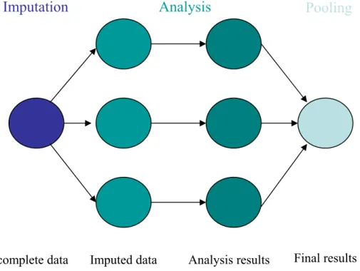
Figure 3.1 – This figure represents all the three phases of multiple imputation.... 67
Figure 4.1 – KM curves for Christie Hospital 1990-94 data set variables’.... 84
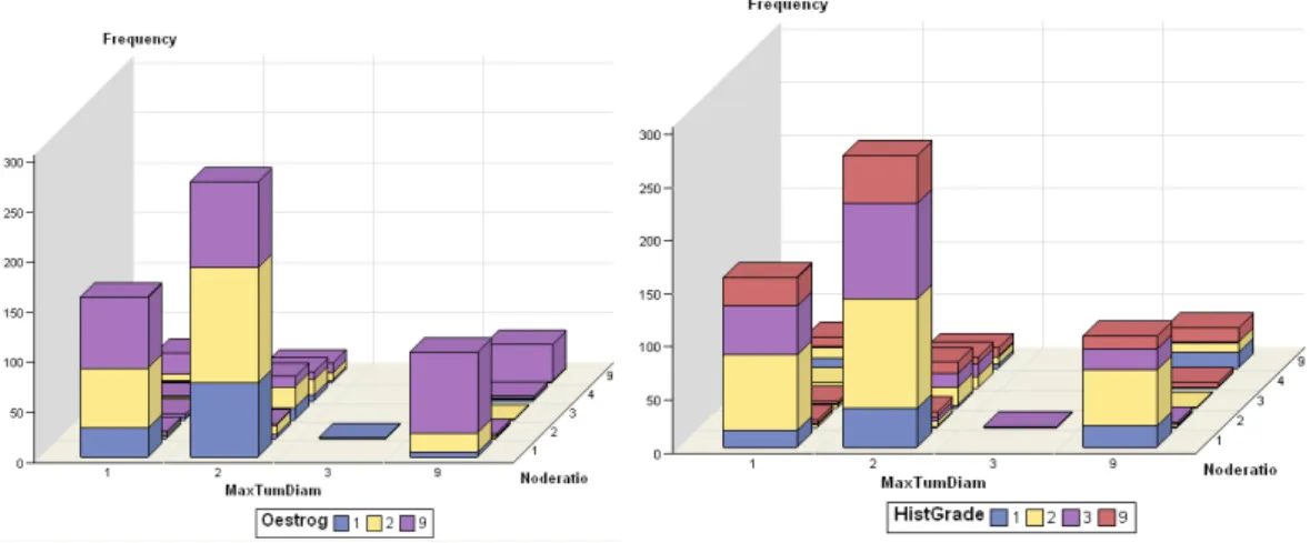
Figure 4.2 – Bar chart comparing the frequency of the categories for different variables..... 85
Figure 4.3 – KM curves BCCA data set variables’.... 87
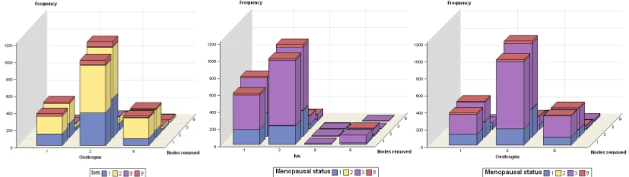
Figure 4.4 – Bar chart comparing the frequency of the categories for different variables..... 88
Figure 4.5 – Scatter plot between the imputed and not imputed model.... 98
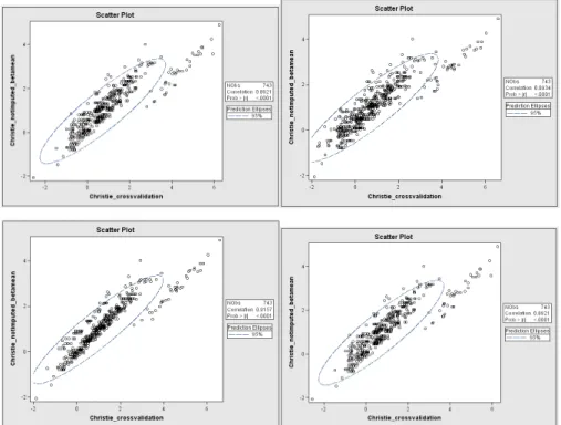
Figure 4.6 – Scatter plot between the cross-validated PI and the PI not cross-validated.... 103
Figure 4.7 – Scatter plot between different prognostic indexes.... 104
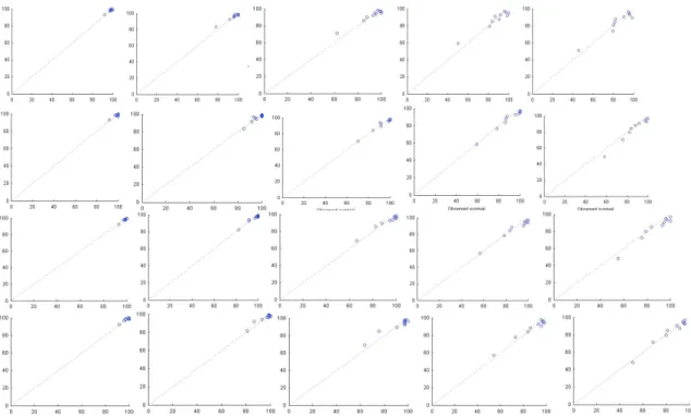
Figure 4.8 – Calibration plots for the 4 different models for the training data set.... 105
Figure 4.9 – Calibration plots for the 4 different models, for the validation data set.... 108
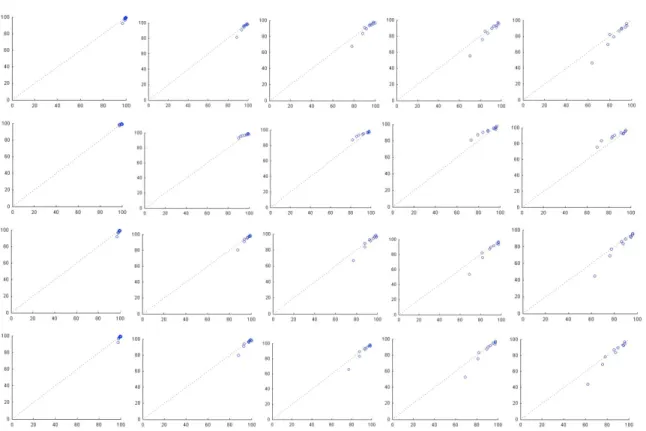
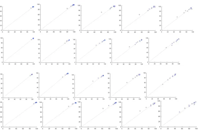
Figure 4.10 – Calibration plots for the 4 different models, for the training data set.... 110
Figure 4.11 – Calibration plots for the 4 different models, for the validation data set.... 111
Figure 4.12 – Comparison between Cox and PLANN-ARD PI for the training data set.... 112
Figure 4.13 – Comparison between Cox and PLANN-ARD PI for the validation data set... 113
Figure 4.14 – Actuarial estimates of survival obtained with KM for the training data set... 115
Figure 4.15 – Actuarial estimates of survival obtained with KM for the validation data set.116 Figure 4.16 – KM curves using the log-rank bootstrapping methodology for both PI.... 118
Figure 4.17 – Final classification tree using the PI obtained with PLANN-ARD.... 123
Figure 4.21 – Box-plots for the different groups....129
Figure 4.22 – KM curves using the regression tree stratification method for both PI....130
Figure 4.23 – Concordance plot for different number of clustering....132
Figure 4.24 – Separation measure (y axis) versus concordance measure (x axis) plot....133
Figure 4.25 – Cramer Area plot....133
Figure 4.26 – Box plots for the 3 (top figures) and 4 (bottom figures) cluster solution....134
Figure 4.27 – KM curves the 4 cluster solution....134
Figure 4.28 – KM curves for the 4 cluster solution, using the validation data set....137
Figure 4.29 – KM curves and cluster in the space of two prognostic indices....138
Figure 4.30 – Cluster projections on different components....139
Figure 4.31 – Survival curves obtained for the patients’ cross-tabulation....141
Figure 4.32 – Survival curves obtained for the patients’ cross-tabulation....142
Figure 4.33 – Survival curves obtained for the patients’ cross-tabulation....144
Figure 4.34 – Survival curves obtained for the patients’ cross-tabulation....145
Figure 4.35 – Survival Distribution for an individual patient....148
Figure 4.36 – Box plots of individual survival estimates to 5 years....148
Figure 4.37 – KM survival curves for the NPI....150
Figure 4.38 – Matrix of KM curves for NPI vs Cox for the validation data set....151
Figure 4.39 – Matrix of KM curves for NPI vs PLANN-ARD for the validation data set.....152
Figure 4.40 – TNM KM survival curves applied to the Christie Hospital data set....153
Figure 4.41 – Consensus rules agreed by the St. Gallen group KM survival curves....155
Figure 4.42 – KM curves for the different PI calculation for the training data set....157
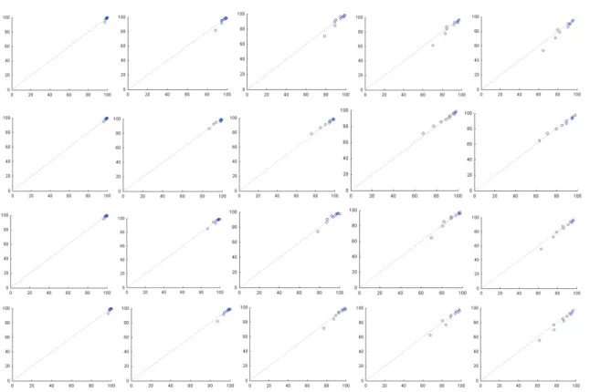
Figure 4.43 – Scatter plots comparing different prognostic indices....159
Figure 4.44 – KM curves for the different four variables models, for the training data set..161 Figure 5.1 – Home page of breast cancer decision support system...171
Figure 5.2 – Home page of breast cancer decision support system after the introduction of a registration user...171
Figure 5.3 – Prognostic assessments for a particular patient....174
Figure 5.4 – Treatments information on the web-site....174
Figure 5.5 – Matrix with KM curves for a patient choosing NPI and PLANN-ARD....175
Index of Tables
Table 2.1 – Example for a Kaplan-Meier curve calculation... 16
Table 2.2 – Example of s inputs and outputs for the PLANN-ARD model.... 37
Table 2.3 – St. Gallen risk categories 2007.... 58
Table 3.1 – Relative efficiency of multiple imputation.... 68
Table 4.1 – Variables’ description and marginal distributions.... 79
Table 4.2 – Continuation of variables’ description and marginal distributions.... 80
Table 4.3 – Continuation of variables’ description and marginal distributions.... 81
Table 4.4 – Cross tabulations between some Christie Hospital variables.... 85
Table 4.5 – Missingness associations for Christie Hospital data set.... 86
Table 4.6 – Missingness associations for the BCCA data set.... 88
Table 4.7 – Results of the missing data imputation with 10 and 20 iterations.... 90
Table 4.8 – Missing data imputated compared with original data for both data sets.... 91
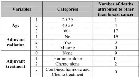
Table 4.9 – Relation between the event other causes of death and some variables.... 93
Table 4.10 – Models chosen using the bootstrapping ordered by their frequency.... 94
Table 4.11 – Beta values for Cox proportional modelling... 94
Table 4.12 – -2LogL statistic for different fitted models.... 95
Table 4.13 – Models parameters for the imputed data sets.... 96
Table 4.14 – Models parameters for the not imputed data sets.... 97
Table 4.15 – Beta values comparison for imputed and not imputed model.... 99
Table 4.16 – Imputation results comparison.... 101
Table 4.17 – Models chosen using bootstrapping, coding missing as a different attribute.. 101
Table 4.18 – Models chosen using bootstrapping applied to the imputed data sets.... 102
Table 4.19 – Models Calibration and discrimination assessment.... 105
Table 4.20 – Models Calibration and discrimination assessment.... 107
Table 4.21– Models Calibration and discrimination assessment.... 109
Table 4.22 – Models Calibration and discrimination assessment.... 110
Table 4.23 – Log rank pairwise comparisons for the validation data set.... 117
Table 4.24 – Log-rank pairwise values for the different risk groups.... 119
Table 4.28 – Mean KM survival values at the end of follow up (5 years)....122
Table 4.29 – Log-rank pairwise values for the different risk groups....126
Table 4.30 – Rules obtained with regression tree using the Cox proportional hazards PI...127
Table 4.31 – Rules obtained with regression tree using the PLANN-ARD PI....128
Table 4.32 – Mean KM survival values at the end of follow up (5 years)....129
Table 4.33 – Log-rank pairwise values for the different risk groups....131
Table 4.34 – Log-rank pairwise values for 4 cluster solution....135
Table 4.35 – Rule-based characterization of the patient cohorts....135
Table 4.36 – Patients’ cross tabulation using the application of nearest records and rules.136 Table 4.37 – Log-rank pairwise values for the 4 cluster solution and validation data set....137
Table 4.38 – Log-rank pairwise values for the 5 cluster solution...138
Table 4.39 – Patients’ cross tabulation between two different stratification methodologies.140 Table 4.40 – Risk groups’ cross tabulation between different models....143
Table 4.41 – Mean and 95% confidence intervals....148
Table 4.42 – Cross-tabulation between different classification schemes....150
Table 4.43 – Log-rank pairwise values for TNM applied to the training data set....153
Table 4.44 – Cross-tabulation between different classification schemes....153
Table 4.45 – Risk group consensus rules agreed by the St. Gallen group....154
Table 4.46 – Cross-tabulation between different classification schemes....155
Table 4.47 – Cross tabulations between different PI calculations for the training data set..158 Table 4.48 – Cross tabulation between patients’ risk group allocation....160
Table 4.49– Distribution of the different treatments for the different risk groups....162
Table 4.50 – Distribution of the different treatments for the different risk groups....162
Table 4.51 – Distribution of the different treatments for the different risk groups....162
Table 4.52 – Higher Treatments’ Risk group Ratio for different models, for the training data set....163
Table 4.53 – Distribution of the different treatments for the different risk groups....163
Table 4.54 – Distribution of the different treatments for the different risk groups....164
Table 4.55 – Distribution of the different treatments for the different risk groups....164
Table 4.56 - Higher Treatments’ Risk group Ratio for different models, for the validation data set....164
Chapter 1
-Introduction
Predictions of the prognosis for a patient diagnosed with cancer has an important clinical role in informing decisions on the choice of adjuvant therapy, in particular to minimise the risk of under- or over-treatment. Current interest in the development of personalised medicine increasingly requires the specialisation of clinical outcome predictions at the level of the individual patient. Moreover, patient empowerment for “shared decision-making” makes physicians and patients both active participants in deciding on the choices for therapeutic interventions. This requires accurate communication and transparent explanations about the prognosis of the disease, in order to permit a well-founded assessment of the risks and benefits of particular treatment choices. In clinical practice, prediction models inform patients and their physician on the probability of a diagnosis or a prognostic outcome as well as stratifying the patients according into risk groups, which can be useful for communication between physicians. Stratification is also important for promoting consistent care protocol between physicians and in the design and assessment of clinical trial outcomes by comparing like-for-like patients.
However, it is imperative for the application of the model that its predictions are reliable, quantifying how accurate the predictions from the model are, which is the “Model Performance”. Furthermore, the gold standard for performance evaluation is to carry out an external validation, that is to say predicting for patients from a clinical centre that is different from the clinical centres from which patient data were acquired for model development (Lisboa, 2002).
There are several clinical prognostic classification schemes proposed for breast cancer patients, some of which discriminate between the survival of different risk groups defined from the patient characteristics. A general criterion defined by the World Health Organisation is the so-called Tumour, Nodes and Metastasis (TNM) staging system, which is a rule-based filter whose arguments are the ordinal representations of tumour size (T), the extent of spread of the disease to the lymph nodes (N) and the presence of clinical signs of metastatic spread (M). The strength of this index is that it only requires clinical information, which is obtained by the clinician without resort to laboratory tests.
A limitation of TNM staging is that its discrimination power is best for separating severe from early-stage disease. Clinically, it is important to differentiate between the severity of illness of patients with non-metastatic disease, sometimes referred to as the ‘operable group’ since, for them, there is the possibility of completely removing the cancer. However, this requires the addition of histological information about the stage of advancement of the cancerous tissue cells. This is provided in one of the most widely used early stage clinical indices for breast cancer, the Nottingham prognostic index (NPI) (Haybittle, Blamey, Elston, Johnson, Doyle, Campbell, Nicholson, Griffiths, 1982). This index combines the pathological size of the tumour, measured in cm, together with an integer index of histological grade in three discrete groups (good, moderate and poor differentiation) and the number of axillary lymph nodes affected, also in three groups.
Note that this index comprises a linear combination of discrete categories, forming an analytical scoring index which can be represented as β.x in a Cox regression model. The second point to note about this robust and time honoured score is that is relies on a careful non-uniform discretisation of the categorical variables of histology and nodes affected. It is therefore a non-linear index, albeit expressed linearly in terms of discrete indicators. The model was fitted to explain the variation in survival, lending itself naturally to the derivation of a discrimination index that has since undergone extensive multi-centre validation (Galea, Blamey, Elston, Ellis, 1992).
Prognostic indexes have been proposed both as a continuous score, providing a risk estimate for individual patients, and on a discrete basis, for defining a limited number of risk groups from which non-parametric grouped survival estimates can be obtained, for instance using Kaplan-Meier, or actuarial, methods. A further score is the consensus rules agreed and
More recently, there was much interest in deriving predictive indices to estimate the likely survival of individual patients, rather than discriminating between different risk groups. One such model is AdjuvantOnline (Ravdin, Sminoff, Davis, Mercer, Hewlett, Gerson, Parker, 2001), which goes further than pure prognosis and reports also the impact on 10-year survival from different choices of adjuvant therapy. This model is derived from meta-analysis, rather than by fitting a single empirical data set from a longitudinal cohort study, although it has been validated using the same cohort with 10-year follow-up that serves as the reference data set for this study (Olivotto, Bajdik, Ravdin, Speers, Coldman, Norris, Davis, Chia, Gelmon, 2005). However, it does not report confidence intervals for its predictions.
Although the final power of any index is limited by the substantial unexplained prognostic heterogeneity and the data accuracy of the adopted retrospective databases, it is relevant to ask whether a generic non-linear database methodology can be developed. This will remove the need to limiting assumptions such as the proportionality of hazards in Cox regression and to remove also the need to discretise continuous variables in order to obtain piecewise linear models using linear-in-the-parameter methodologies. These models have the potential to provide better accuracy than traditional methodologies because of their flexibility due to a semi-parametric formulation using distributed nodes, in the case of artificial neural networks. Clearly the generalisation of the model needs to be controlled with a robust regularisation framework and evaluated empirically with a carefully designed external validation study.
This thesis evaluates the possible advantages of a non-linear, time dependent neural network methodology for survival modelling of a single risk, or outcome. This is the Partial Logistic Artificial Neural Network regularized with a Bayesian network using a Laplace approximation of the evidence, known as Automatic Relevance Determination (MacKay, 1995), hence PLANN-ARD. In particular, the thesis reports the first large-scale performance evaluation of this methodology for an external data set, using imputation and risk stratification. This is benchmarked with the stalwart linear model for survival, Cox regression. According to an easier interpretation of covariate effects, the non-linearities that are inherent in outcome modelling of medical data are often naïvely taken into account implicitly by collecting real-valued covariates binned into discrete groups. Consequently, in such a framework, a flexible model such as the neural network can only improve modelling accuracy by implicitly modelling additive (interactions) effects between covariates and non-proportional covariate effects, which in linear models need to be parameterised explicitly.
The PLANN-ARD model takes account of censorship that occurs when a patient drops out of the study before the event of interest is observed, for instance being lost to follow-up without a definitive outcome being recorded.
A related matter of clinical relevance is the choice of outcome to model, i.e. the choice of risk. In general there are three possibilities, for breast cancer. The most generic and best defined risk is that of overall mortality, since this a well-defined endpoint in prognostic assessment. It has the limitation of combining together the effects of breast cancer and age-related mortality. However, the alternative of specifying breast specific death suffers from potential inaccuracies in the attribution of the cause of death, for instance in the case of patients who die from a heart attack which may potentially reflect the health load resulting from radiotherapy to the left side of the chest or the toxicity of chemotherapy. A third possibility is to track local and distal recurrences of the disease. This represents multiple competing risks and suffers from potential bias because of the absence from the available databases of follow-up for the occurrence of second primary tumours. Taking all of these factors into consideration, current prognostic decision support systems such as Adjuvant report overall or relative mortality. This thesis focuses on the primary modelling stage for both of these outcome indicators, which is the risk of overall mortality as a function of age and clinical and histological measurements specific to breast cancer.
This thesis also takes in account with the important issue of variable selection by making a carefully analysis in order to incorporate the best predictors of the outcome variables given the cohort sample size.
In addition to the above issues, routinely acquired data from clinical practice commonly contain missing values. Moreover, the data is not missing at completely at random since there may be a reason for missing, for instance because the variables concerned are of no consequence to the choice of therapy. So it is that the survival of the patient group with a particular variable missing do not always lie between the survival groups for extant values, but sometimes are close to the extremes of survival. However, the data used is missing at random, in the sense that the missing can be reasonably imputed from ancillary information, such as the eventual choice of therapy, by representing missing values as random variables (Fernandes, Jarman, Etchells, Fonseca, Biganzoli, Bajdik, Lisboa, 2008). Missing values were incorporated in the benchmark linear model, Cox proportional hazards and the non-linear
When considering out-of-sample predictions it is necessary to distinguish between modelling the training data, which may have missing values; then predicting on an out-of-sample cohort which may also have missing values, possibly in a different set of covariates than the training data, or missing with a different distribution; and predicting for a single new patient, for which data imputation may not be possible. Therefore, this work analyses how these issues can be overcome.
Both prognostic models being compared in this study define a different prognostic index that ranks patient data by severity of the illness that incorporate all the issues mentioned in model developing and were extended to the out-of-sample cohort.
A critical performance indicator in the validation of prognostic models, is the assessment of discrimination and calibration accuracy, both of which are highly relevant in decision support. This performance assessment is carried out in two different ways. First, by a detailed analysis of the predicted vs observed survival over the five years of follow-up for the training data. Second, a prognostic index is defined, with which to assess the discrimination between patient groups, to be evaluated against the crude empirical event rate over the full follow-up period for the validation data, which has a 10 year timeframe.
Once the risk score is defined, the population of patients at risk needs to be stratified for the purpose of tailoring adjuvant therapy and to enable comparisons to be made between patient cohorts from different clinical centres, or subject to different clinical interventions, to be made between patients at similar risk by outcome. This involves the application of significance tests, which in survival analysis is usually the log-rank statistic. However this statistic finds the different patient risk groups by thresholding only the Prognostic Index, making an assumption that the threshold separates distinct patient populations, while in practice it may be cutting across a single patient population. It would be desirable to stratify by identifying distinct patient populations directly from the prognostic factors. Therefore, this thesis make an analysis between 4 different stratification methodologies: the first is a log-rank bootstrap aggregation methodology, which uses the log-rank statistic at its core but carries out bootstrap re-sampling of the population of prognostic indices in order to gain robustness over a maximum significant search. The second methodology is based on regression trees, applied to the continuous value prognostic scores. The third methodology is a robust unsupervised clustering methodology that uses k-means where only patient covariates without any
knowledge of outcome are considered. The fourth one uses informed clustering based on the principle of learning metrics.
Models were trained on a cohort of patients with operable breast cancer recruited at Christie Hospital, Manchester, between 1990-93 (n=743) and were the subject of an external predictive evaluation for overall mortality by applying the model to a database acquired by the British Columbia Cancer Agency (BCCA), Vancouver, during the period 1989-93 (n=4,016).
This study also enhances the existing classification schemes proposed for breast cancer previously mentioned, by comparing them with the PLANN-ARD and Cox proportional hazards modelling followed by a robust stratification methodology. The survival for patient sub-groups was compared for the different methods, revealing the heterogeneity among the prognostic groups of the existent classification schemes. An advancement achieved by PLANN-ARD is to reliably stratify the NPI group 3 of breast cancer patients, which is thought to contain a mixture of patient groups with different severity of illness. The results reported in the thesis identify three sub-groups with statistically different 5 year survival.
Finally, a web decision support system for breast cancer patients was developed in order to incorporate patient’s risk group models, such as the known NPI, the Cox proportional hazards prognostic index and the PLANN-ARD prognostic index both followed by a stratification methodology. The derived explanatory rules, the different treatments received by patients and the KM survival curves were also incorporated to help on the visualisation of relevant existing patient data an interpretation of inferences in clinical terms. It is important to mention that the aim of the proposed decision support system is to enhance the oncologists’ current practices, rather than to replace them. In this decision support framework, the predictive model represents an analytical window into the evidence base comprised of historical patient records. In particular, the model serves to provide a context for the patient, using the risk score and risk group strata, as well as an individualised inference of the expected prognostic outcome, through the predicted hazard for that patient.
Chapter 2 of this thesis presents an overview of the classical survival models and flexible models, including the semi-parametric linear model and PLANN-ARD model, explaining how it can be applied to prognostic modelling. It also describes the existing and proposed stratification methodologies as how Boolean rules extraction can be achieved. In addition,
Chapter 3 starts by outlining the main issues that must be taken in account while developing prediction models which were introduced and analysed in this work. Secondly, it defines how the predictive accuracy and validation must be analysed and the modelling strategy that must be taken in account when developing prognostic models.
Chapter 4 describes the validation results obtained with the flexible modelling approach. It begins with an explanation of the two datasets used for training and external validation and a study of the missing data and the application of multiple imputation. Second, the integration of the multiple imputation into the linear and non-linear modelling methodologies is described, leading to the evaluation of the predictive performance for the two alternative models, each applied to an external validation data set which was not used at all during the optimisation of model fitting to the training data, and in fact from a completely different patient sample, recruited in a different country. The results from the different stratification methodologies, applied to the proposed prognostic models are presented and compared. Finally the relative validation performance of the existent and new prognostic and risk stratification schemes is presented, explaining how these new methodologies can improve those currently used in clinical practice.
Finally, chapter 5 presents an overview of the existing online breast cancer prognostic models, with particular emphasis the AdjuvantOnline. It also defines the web clinical decision support system for breast cancer patients that incorporates the prognostic models proposed in this thesis.
1.1 -
Contribution of the thesis
The present thesis makes an important contribution to both technical innovation and clinical application as several important novelties were added or changed to current practice. Currently there are several survival models which are in use described previuosly, such as NPI and other Cox proportional hazards models. It is intended to augment NPI by adding more variables considered to be important in the prognostic model. Moreover, it was intended to define a prognostic model to become predictive rather than explanatory as well as modelling non-linear dependences, with PLANN-ARD.
This thesis also takes account of missing data and censorship within principled frameworks, applying multiple imputation in combination with neural network models for time-to-event modelling, where a new prognostic index was also considered, which able the stratification of patients into risk groups.
Moreover a new stratification methodology was developed, based on decision trees, which adds a more robust path to identify the patient’s risk group and the explanatory rules that characterize risk group membership, based on patient’s characteristics. Flexible modelling, incorporating the missing data was also subjected to a very accurate validation.
Finally, a new web decision support system contributes to technical innovation as it implements both the previously mentioned models, where all can be compared.
1.2 -
Articles accepted
“Assessment of benefit vs. risk of drug therapy: the potential for outcome analysis with flexible models”, accepted at “2010 International Joint Conference on Neural Networks”, Barcelona (Spain), 18-23 July 2010, Lisboa, P.J.G, Fernandes, A.S., Fonseca, J.M., Bajdik, Chris, Biganzoli, Elia.
“Cohort-based Kernel Visualisation with Scatter Matrices”, accepted at “2010 International Joint Conference on Neural Networks”, Barcelona (Spain), 18-23 July 2010, Romero, Enrique, Fernandes, A.S., Mu, Tingting, Lisboa, P.J.G.
“A clinical decision support system for breast cancer patients”, accepted at “Doctoral conference on computing, electrical and industrial systems”, Lisboa (Portugal), 22-24 February 2010, Fernandes, A.S., Alves, Pedro, Jarman, Ian H., Etchells, Terence A. , Fonseca, José M., Lisboa, Paulo J. G..
“p-Health in breast oncology: a framework for predictive and participatory e-systems”, accepted at “International Conference on "Developments in eSystems Engineering" (DeSE '09)”, Abu Dhabi (United Arab Emirates); 14-16 December 2009; Fernandes, A.S., Bacciù, D., Etchells, T.A., Jarman, I.H., Fonseca, J.M., Lisboa, P.J.G.
“Different methodologies for patient stratification using survival data”, accepted at “Sixth International meeting on computational intelligence methods for bioinformatics and biostatistics”, special session “Intelligent systems for medical decisions support (ISMDS)”; Génova (Italia); 15-17 October 2009; Fernandes, A.S., Bacciù, D., Etchells, T.A., Jarman, I.H., Fonseca, J.M., Lisboa, P.J.G.
“Evaluation of missing data imputation in longitudinal cohort studies in breast cancer survival”; Int. J. Knowledge Engineering and Soft Data Paradigms, Vol. 1, No. 3, 2009, pp. 257-276; Fernandes, A.S., Etchells, T.A., Jarman, I.H., Fonseca, J.M., Biganzoli, Elia, Bajdik, Chris, Lisboa, P.J.G.
“Stratification methodologies for neural networks models of survival”, Proceedings of the 10th International Work-Conference on Artificial Neural Networks (IWANN2009), Salamanca, Spain; vol. 5517 – Pág. 989-996; Springer (2009); Fernandes A.S., Etchells T.A., Jarman, I.H., Fonseca, J.M., Biganzoli, Elia, Bajdik, Chris, Lisboa, P.J.G.
“Missing data imputation in Longitudinal Cohort studies – Application of PLANN-ARD in Breast cancer Survival”; The 7th International Conference on Machine Learning and Application (ICMLA’08), Vol. 5177, pp. 214-221, Springer (2008); San Diego, California; Fernandes, A.S., Etchells, T.A., Jarman ,I.H., Fonseca, J.M., Biganzoli, Elia, Bajdik, Chris, Lisboa, P.J.G.
“Stratification of severity of illness indices: a case study for breast cancer prognosis”; Proceedings of the 12th International Conference on Knowledge-Based and Intelligent Information & Engineering Systems (KES'08), Zagreb,Croatia; vol. 5178 – Pág 214-221; Springer; Etchells T.A., Fernandes, A.S., Jarman, I.H., Fonseca J.M.,Lisboa P.J.G.
“Stratification of severity of illness índices and out-of-sample validation: a case study for breast cancer prognosis”, chapter in “Computational Intelligence in Human Cancer Research”; KES Rapid Research Results Series; Etchells, T.A., Fernandes, A.S., Jarman, I.H., Fonseca, J.M., Lisboa, P.J.G.
Chapter 2 -
Analytical methodologies
This chapter introduces the survival models and artificial intelligence techniques used in this thesis and it is divided in four different sections. The first section gives an overview of classical survival methods, which explains in detail the benchmark model used in this thesis, the Cox proportional hazards modelling. The second section describes flexible models and how these can incorporate survival analysis, introducing the PLANN-ARD model, which is used in this thesis. This chapter also provides a description of the stratification methods that can be applied to a prognostic index obtained with survival modelling. Finally, an overview of clinical prognostic indexes is presented, making a higher emphasis on the existing prognostic indexes in breast cancer field.
2.1 -
An overview of classical survival methods
Survival Analysis is composed by statistical methods used to study the occurrence and timing or the events. It analyses the data from a specific time of origin until the occurrence of a particular event. These methods were designed to apply in the study of deaths. However, the survival analyses can be applied in other kind of events, such as equipment failure, automobile accidents, stock market crashes, job terminations, births, marriages, divorces, arrests, and other.
In medical research, the time origin corresponds to the recruitment of the individual and the end-point can be the death of the patient, relief of pain, recurrence of symptoms. The result of the first end-point referred is literally survival times.
Survival analysis was designed for longitudinal data on the occurrence of events, and it is very important to clarify the events in the study. The event can be characterized as a qualitative change (transition from one state to another, such as being alive to being death) and a quantitative change (a stock market crush could be defined as a single day life loss of more than 20% in the market index). However, in survival analysis it is needed to know more than a qualitative or a quantitative change. You also have to situate this event on time.
The survival analysis can be performed considering only the time of events, but a usual aim of these methods is to estimate causal or predictive models in which the risk of an event depends on the covariates These covariates can be constant over the period of study, such as sex and race, or can change over the period of study, such as age, blood pressure, marital status. There are some reasons to consider why survival data can’t be obtained with conventional statistical procedures. The first one is related with the fact that survival data is not symmetrically distributed and consequently this type of data does not have a normal distribution. Transforming the data to give a more symmetric distribution could solve this feature. However, a more satisfactory approach is to adopt alternative distributional model to the original data.
Besides this feature, the survival data has also other two features that are difficult to handle with conventional statistical procedures, which are censoring and time-dependent-covariates. The following example illustrates both problems: a sample of X prisoners was followed one year after release. The event of interest is the first arrest and the aim of the study is to determine how the occurrence and timing of arrest depends on some covariates. Some of these covariates are constant during the period of study, such as sex or race, others could change ate any time during the period of follow-up. How can this data be analysed using conventional methods? The conventional methods ignore the information about timing of arrest. Ignoring this information should reduce the precision of the estimates. One solution to this problem is to make the dependent variable the length of time between the release and first arrest and then estimate a conventional linear regression model. But what can be made with the persons who were not arrested during the follow-up period? Such cases are called
Another problem is how to deal with a time-dependent variable, such as employment status. This variable can be incorporated in the data estimating 52 indicator variables (one variable for each week indicating the employment status). This can lead to a computational awkwardness and statistical inefficiency. Aside to this, there is a more fundamental problem, such as the employment indicators for weeks after an arrest might be a consequence of the arrest rather than the cause. In particular, someone who is jailed after an arrest is not likely to be working full time in subsequent weeks.
In conclusion we can say that conventional methods are not efficient dealing either with censoring and time-dependent covariates. However, the survival analysis methods allow censoring, and many also allow time-dependent covariates.
2.1.1.Censorship and their importance
Censorship is the main feature of survival analysis. The survival time of an individual is said to be censored, not only when the end-point of interest has not been observed for that individual but also, if at the end of the study the individual has not experienced the event. During the follow-up it is necessary to know if the event has occurred or not and when did it occur. Sometimes, the survival status of an individual cannot be known, as that individual has been lost to follow-up. For example, consider that the recruited individual, after being recruited, moves to another country and his survival experience cannot be traced. The only information available is the last date he or she was known to be alive.
Another reason for a survival time being considered censored is when the event experienced is different from the event of interest, which happens due to a cause that is known to be unrelated to the specific study. However, this type of censoring is difficult to be sure that is not related to the study. For example, consider a patient in a clinical trial to compare alternative therapies for prostatic cancer who experiences a fatal road traffic accident. The accident could have resulted from a side effect of the treatment. If so, the death is related with the treatment and cannot be considered censored. A breast cancer patient who dies due to a cause unrelated with the disease, has to be considered censored. This kind of event is known as competing risk events. Suppose also that a breast cancer patient undergoes a prophyletic oophorectomy after surgery to breast cancer. This prophyletic treatment substantially reduces the probability of developing ovarian cancer. So it is considered a competing risk event when calculating ovarian cancer incidence. A competing risk may
preclude the onset of the event of interest, or may modify the probability of the event of interest. An individual who experiences a competing risk event is censored in an informative manner. However it is necessary to analyse the data and the event of interest to conclude if the informative censoring makes any influence in the estimate of the probability of the event of interest. If it does not make any influence, the informative censoring can be ignored. For example, death to other causes may not be related to having breast cancer unlike breast cancer-specific mortality. Here, the informative censoring does not influence the estimates of breast cancer mortality. It is important to verify if censoring is noninformative, because otherwise a bias is introduced in survival analysis methods. Resuming, good patient follow-up and avoidance of unnecessary drop-out is the best solution (Bradburn, Clark, Love, Altman, 2003).
2.1.2.Survivor function and Hazard function
In survival analysis there are two functions of central interest such as the survivor function and the hazard function. The survivor function represents the probability that an individual survives from the time origin to some time beyond t:
S(t)=P(T≥t) (1)
The hazard function is widely used to express the risk or hazard of an event at time t, and is obtained from the probability that an individual experience the event at time t, conditional on he or she having survived to that time:
h(t)=lim δt→0 P(t≤T <t+δt |T ≥t) δt ⎧ ⎨ ⎩ ⎫ ⎬ ⎭ = f(t) S(t) (2) where f(t)= dF(t) dt (3) and F(t)=Pr(t≤T)= f(u)dt =1−S(t) t=0 T
∫
(4)This function can also be called hazard rate, instantaneous death rate or force of mortality and represents the approximate probability that an individual dies in the interval (t,t+δt),
that time. It can vary from 0 to infinity. It can increase or decrease or remain constant over time. The function H(t), called cumulative hazard, can be obtained from the Survivor function, since:
H(t)= −log S(t) (5)
Supposing that in a single sample of survival times none of the observations are censored, the survival function S(t) can be estimated by the empirical survival function, given by:
S(t)= Number of individuals with survival times ≥ t
Number of individuals in the data set
(6)
The estimated survivor function is assumed to be constant between two adjacent death times. The overall survival probability is the probability of being event-free at least up to a given time. The cumulative incidence of an event at a given time is one minus the overall survival probability at that time.
Consider, for example, the event of interest to be death. Suppose that 100 patients lived for at least 1 year and 5 patients died. The estimated survival at 1 year is 95%. Suppose, at 2 years, 10 patients died. The estimated survival at 2 years is 85/95=89,5%. The estimated overall survival probability up to 2 years is the probability of having survived to first and second year, which is 95*89,5=85%. The cumulative incidence of mortality at 2 years is the sum of mortality at first and second years, which is, in the previous example (95/100)+((95/100)*(10/95)) =15%.
2.1.3.Actuarial/Descriptive Model – Kaplan Meier
There are some methods for the estimation of the survival function and the hazard function. Methods for estimating these functions from a single sample of survival data are said to be non-parametric or distribution free, since they do not require a specific assumption to be made about the distribution of the survival times.
The Kaplan-Meier approach provides a non-parametric estimate of the overall survival probability of an event of interest. It adequately deals with censored data, and provides attractive graphs on the relationship between predictor values and the outcome over time. The cumulative incidence is calculated as 1 minus this survival probability. Every individual in the data set has a follow-up time and status (event or censored). In order to estimate the survivor function, the follow-up times where an event has occurred are ordered from the
smallest to the largest. Then a series of time intervals are constructed. These intervals begin at the time when an event has occurred and end at the time before the next event occurs. No intervals begin at a censored time. It can be noticed that there can be ties, since more than one individual can die simultaneously.
Considering nj the number of event free individuals up to time tj and dj the events occurred
at time tj, the estimated survival probability at time tj is given by (nj-dj)/nj. The overall
survival probability up to time tj, denoted S(tj) is the probability of surviving up to tj,
including time tj. Therefore the overall survival probability up to tj is the product of the
probability of surviving trough the interval tj-1 to tj and all preceding intervals. Then it can be
said that a product of series of estimated probabilities forms the Kaplan-Meier estimate: S(tj)=S(tj −1)× nj−dj nj (7) S(t)= ni−di ni i=1 k
∏
(8)A plot of the Kaplan-Meier estimate of the survival function is a step-function, where the estimated survival probabilities are constant between adjacent death times and decrease at each death time. In the absence of censoring the Kaplan-Meier estimate is simply the empirical survivor function. Therefore, it can be concluded that the Kaplan-Meier estimate is a generalisation of the empirical survivor function that accommodates censored observation.
In the following example it can be observed how the Kaplan-Meier curve is calculated:
Time interval Hazard at the beginning of interval Censored during the interval Hazard at the end of interval Deaths in
the interval Survival at the end of interval Overall survival at the end of interval
0-1 7 0 7 1 6/7=0,86 0,86
1-4 6 2 4 1 ¾=0,75 0,86*0,75=0,64
4-10 3 1 2 1 ½=0,5 0,86*0,75*0,5=0,31
10-12 1 0 1 0 1/1=1 0,86*0,75*0,5*1=0,31
Figure 2.1 – Example of a Kaplan-Meier curve
When competing risk events are present in the data, it is necessary to make some considerations about the Kaplan-Meier estimate. Satagopan et al (Satagopan, Ben-Porat, Berwick, Robson, Kutler, Auerbach, 2004) makes some illustrations of a non-parametric estimation of the cumulative incidence function for an event of interest in the presence of competing risk events
2.1.4.Piecewise Linear Models – Proportional Hazards (Cox regression Model)
The actuarial or descriptive methods described can be useful in the analysis of a single sample of survival data or in the comparison of two or more groups of survival times. However, in most studies, supplementary information (explanatory variables) is also recorded for each recruited individuals. The analysis, using this information is much more complex than the analysis considered before. In order to analyse the relationship between the survival experience and the explanatory variables of the individuals it is used an approach based on statistical modelling. There are two main reasons for modelling survival data. First, one objective of the modelling process is to determine how the explanatory variables affect the hazard function. Another objective is to obtain an estimate of the hazard function for an individual, in order to estimate the median survival time. This value can be estimated for current or future individuals with particular values of the explanatory variables.
When the survival times are assumed to follow a statistical distribution, it should be used a fully parametric model. There are different distributions and the identification of a suitable one is a crucial step in modelling the survival data. What distinguishes between the existing
parametric models is the shape of the hazard they assume the data follows. If the hazard is always increasing and decreasing, the Weibull and Gompertz distributions are appropriate. If the hazard rises to a peak and then decreases or always decreases, then the Log-Logistic distribution should be used. Log-Normal or Generalised Gamma models are preferable used when the hazard rises to a peak and then decreases. In the Exponential model, the hazard is constant over time.
If there is no need to assume a particular form of the probability distributions for the survival times S(t), then the Cox regression model is used. In medical studies, the Cox proportional hazards model it the most often used method of survival outcomes. This model is based on the assumption of proportional hazards, that is, assumes that the log(-log (S(t))) for different subjects are equidistant over time or equivalently that the hazard function for any two subjects are proportional over time. Therefore, this model is referred as semi-parametric model.
As stated before, the Cox regression model is based on the assumption of proportional hazards. The following example can explain this property of the model.
Suppose two patients are randomised to receive a standard treatment or a new treatment. hS(t) is the hazard of dead at time t the first treatment and hN(t) is the hazard of the second.
According to the proportional hazards model:
hN(t)=ψhS(t) (9)
This assumption implies that the corresponding true survivor functions for individuals on the new and standard treatment do not cross. The ψ value corresponds to the ratio of the hazards of death at any time for an individual on the new treatment relative to an individual on the standard treatment. The ψ value is known as the relative hazard or hazard ratio.
In the Cox regression model a reference group called the baseline population specifies all time dependence, which is characterized by a zero covariate vector (h0(t)). The values of these covariate will be assumed to have been recorded at the time origin of the study. The set of values of the explanatory variables for each individual will be represented by x. The hazard function can be written as:
As the relative hazard cannot be negative, it can be written has eηp, where ηp is the linear
combination of the explanatory variables of the individuals. This quantity is the linear component of the model and it is also known as the risk score or prognostic index for the ith individual. The dependence of the covariate variables is then aggregated into the scalar βTx
p.
Consequently,the general proportional hazards model is as follow: hp(xp,t)=e(βTx
p)h
0(t) (11)
This model can be re-expressed in:
log hi(t) h0(t) ⎧ ⎨ ⎩ ⎫ ⎬ ⎭ =β Tx p (12)
The hazard function may depend on two types of variables namely variates and factors. A variate is a variable that takes numerical values that are often on a continuous scale of measurement, such as age. A factor is a variable that takes a limited set of values which are known as the levels of the factor, such as the variable gender. If we have a situation where the hazard function depends on two variables, X1 and X2 the proportional hazards for the ith
individual, can be written as:
hi(t)=e
(β1x1+β2x2)h
0(t) (13)
Using this model, the logarithm of the hazard ratio is considered linear, due to: log hi(t) h0(t) ⎧ ⎨ ⎩ ⎫ ⎬ ⎭ =β1x1+β2x2 (14)
Considering the ratio of the hazard of death for an individual with the value x+1 for X relative to one with value x, it obtains:
e{β(x+1)}
eβx =e
β (15)
This ratio shows that when a variable with a single beta is included in the model, the hazard ratio when the value of X is changed by r units does not depend on the actual value of X. This means that the hazard ratio for an individual with value 60 for a variable, related to one with value 55 for the same variable, is the same for an individual with value 20 related to one with value 15 for the same variable. This is a result of fitting X as a linear term in the proportional hazards model.
Supposing that the dependence of the hazard function on a single factor A is to be modelled where A has a levels, the proportional hazards model for an individual with factor A at level j is e(αj)h
0(t) . Here, the baseline hazard function has to be defined as the hazard for an individual with values of all explanatory variables equal to zero. Consequently, one of the
αj must be taken to be zero. If the constraint α1=0 is adopted, the term αjcan be included defining a-1 indicator variables, X2,X3,….Xa, which take the values shown below:
Level of A X2 X3 …. Xa 1 0 0 …. 0 2 1 0 …. 0 3 0 1 …. 0 …. …. …. …. 0 a 0 0 …. 1
For each ith individual it is only possible to have one variable for each factor, and the proportional hazards model can be written as:
hi(t)=e
(β2x2+β3x3+...+βaxa)h
0(t) (16)
Using this model, the logarithm of the hazard ratio is considered piece-wise linear, because each covariate has the number of betas equals to the number of levels that exist.
However, it is important to mention that equation 12 represent the Cox Regression Model in continuous time. When the model is in discrete time equation 12 is re-expressed as in the following equation: x t h t h x h x h +β ⎟⎟ ⎠ ⎞ ⎜⎜ ⎝ ⎛ − = ⎟⎟ ⎠ ⎞ ⎜⎜ ⎝ ⎛ − 1 ( ) ) ( log ) ( 1 ) ( log 0 0 (17)
2.2 -
Flexible Models
2.2.1.Generally of Artificial Neural Networks
An artificial neural network (ANN) is a mathematical model or computational model originally inspired on the central nervous system and neurons.
As described in (Bar-Yam, 1997), the basic computational unit in the nervous system is the nerve itself, or neuron. A neuron has dendrites, cell body and axon. A biological neuron receives input from other neurons. The input zone is composed by the dendrites. When the potential reaches a threshold, the cell fires and an action potential propagates along the axon (output) to other neurons, through an electrical signal. Transmission of an electrical signal from one neuron to the next is affected by neurotransmitters chemicals, which are released from the first neuron and bind to receptors in the second. This link is called a synapse.
Figure 2.2 – Constitution of a neuron (Computation in the brain).
Brain learns by altering the strengths of connections between neurons, and by adding or deleting connections between neurons. Brain learns based on experience, which means that connexions between neurons are dynamic. Connexions highly used are strengthened and connexions less used tend to disappear. The same phenomenon happens in neural networks.
There are several properties of the nervous system that are of particular interest in the biologically inspired Neural Networks models, which are:
1. Parallel and distributed information processing 2. High degree of connectivity among basic units 3. Connections are modifiable based on experience 4. Learning is a constant process
5. Learning is based on local information
6. Performance degrades gracefully if some units are removed
The basic computational element (model neuron) is often called a node or unit. It receives input from other units or from an external source. Each input has an associated weight w, that is modified while the model learns. The “electrical” information is simulated using numerical values stored in these weights. The unit computes a function f of the weighted sum of its inputs. This resembles the perceptron model of Rosenblatt (1962), which is a linear discriminant model. In a simplistic neural network the summed value is compared with a certain threshold, in order to propagate the signal or not. However nowadays, instead of a threshold activation functions are used. Using the perceptron of Rosenblatt the nonlinear f
function is given by the step function and the algorithm used to determine the parameters w of the perceptron is an error function known as the perceptron criterion.
yi= f(
∑
wijxj) (18)Figure 2.4 – Example of a perceptron.
Σ
f
y
i
x1 . . . xj x0 = 1 (bias)The output can serve as the input to other units. The function f(x) is the unit’s activation function. This activation function describes the output behaviour of a neuron. There are several activation functions that can be used. The choice of the activation function is determined by the nature of the data and the assumed distribution of target variables. Activation functions for the hidden units are needed to introduce nonlinearity into the network. Without nonlinearity, hidden units would not make nets more powerful than just plain perceptrons (which do not have any hidden units, just input and output units). The reason is that a linear function of linear functions is again a linear function. However, it is the nonlinearity (i.e., the capability to represent nonlinear functions) that makes multilayer networks so powerful. Almost any nonlinear function does the job, except for polynomials. Following are some of the commonly used activation functions:
Figure 2.5 – Representation of possible neural networks activation functions.
The top pictures are from left to right, the step, identity and sigmoid function, respectively. The bottom pictures are the symmetric sigmoid function and the radial basis functiony.
If several perceptrons or weighted neurons are connected to each other, i.e., the output of a perceptron is the input of another perceptron, there will be a neural network model, or also known a multilayer perceptron or MLP. In a MLP the neurons are organized in layers, which number differs from network to network. The input nodes receive signals from “outside” the network and the output nodes send the signals “outside” the network. If there is a layer
constituted by several nodes, but their signals are not received from outside the network nor are sent to outside the network, then it is called hidden layer. A multilayer perceptron have several hidden layers, some input nodes and some output nodes, which is represented by the following figure:
Figure 2.6 – Example of a multilayer perceptron. It has 1 hidden layer, 3 input nodes and 2 output nodes
The weight parameters are represented by the links between the nodes and the arrows denote the direction of information that flows through the network during forward propagation. There was however introduced a new element, called “bias”, which defines the neuron trend, subject to modifications during the network training. Bias units can also be weighed and connect an unitary input to each neuron.
The number of neurons on each layer is always equal to the number of variables. Although the number of hidden layers may differ, it is almost always equal to two or three. This is a result of a study done by Bishop (Bishop, 2006), where he shows that any network with two hidden layers can approximate any function independently of its complexity. One the one hand we should consider to use always a powerful network (three layers), on the other hand this network can create overfitting problems (there is a lost of a generalisation capacity).
Combining these various stages to give the overall network function, using sigmoidal output activation, the final network takes the form:
yk(x,w)=σ wkjh wjixi+wj0 i=1 N