Concurrency, Specification
& Programming
24th International Workshop, CS&P 2015
Rzeszow, Poland, September 28-30, 2015
Proceedings
Volume 1
Editors
Zbigniew Suraj Ludwik Czaja
Chair of Computer Science Institute of Informatics University of Rzeszow University of Warsaw
Rzeszow and Vistula University
Poland Warsaw
Poland
This two-volume book contains the papers selected for presentation at the Concurrency, Specification and Programming (CS&P) Workshop. It is taking place from 28th to 30th September 2015 in Rzeszow, the biggest city in southeastern Poland.
CS&P provides an international forum for exchanging scientific, research, and tech-nological achievements in concurrency, programming, artificial intelligence, and related fields. In particular, major areas selected for CS&P 2015 include mathematical models of concurrency, data mining and applications, fuzzy computing, logic and probability in theory of computing, rough and granular computing, unconventional computing mod-els. In addition, three plenary keynote talks were delivered.
The Workshop was initiated in the mid-1970s by computer scientists and mathe-maticians from Warsaw and Humboldt Universities, as Polish-German annual meetings. The first meeting in this series was named 1st Symposium on Mathematical Foundations of Computer Science and it took place in Warsaw from 12th to 19th September 1976. These meetings have been suspended for some years in the eighties until the beginning of ninetieths, and reactivated in 1992. Since then, the Workshop bears the name CS&P, when the first meeting after the break came into effect in Berlin. Now, it is being orga-nized every even year by the Humboldt University of Berlin and every odd year by the University of Warsaw.
It should be mentioned that the CS&P meetings, initially purely bilateral, since 1992 have developed into events attended by participants from a number of various countries beside Poland and Germany. In 2003 the University of Information Technol-ogy and Management in Rzeszow, in 2004, the Fraunhofer Institut FIRST in Berlin, and in 2015, the University of Rzeszow jointed the organizers as full members of the Committee and financial contributors. The present CS&P 2015 meeting will be host-ing participants from the followhost-ing countries: Canada, Germany, India, Italy, Poland, Russia, Saudi Arabia, Slovakia, Ukraine.
The CS&P 2015 is the twenty-fourth meeting after the break. It received 53 submis-sions that were carefully reviewed by Program Committee members or external review-ers. After a reviewing process, 49 papers were accepted for presentation at the workshop and publication in the CS&P 2015 proceedings. This book also contains three extended abstracts by the plenary keynote speakers.
It is truly a pleasure to thank all those people who contributed to preparation of this book. In particular, we would like to express our appreciation for the work of the CS&P 2015 Program Committee members and external reviewers who helped to assure the high standards of accepted papers. We would like to thank all the authors of CS&P 2015, without whose high-quality contributions it would not have been possible to or-ganize the workshop. We are grateful to the Organizing Committee members for their involvement in all the organizational matters related to the CS&P 2015 as well as the creation and maintenance of the conference website. We wish to express our thanks to Mikhail Moshkov, Andrzej Skowron and Louchka Popova-Zeugmann for accepting to be plenary speakers at CS&P 2015. We greatly appreciate the financial support received
II
from the University of Rzeszow, the University of Warsaw, and the Vistula University in Warsaw.
We hope that the CS&P 2015 workshop proceedings will serve as a valuable refer-ence for researchers and developers in the field.
September 2015 Zbigniew Suraj
CS&P 2015 was organized by the Chair of Computer Science, the University of Rzes-zow, RzesRzes-zow, Poland, in cooperation with the Institute of Mathematics and the Insti-tute of Informatics, the University of Warsaw, Warsaw, Poland, the Vistula University, Warsaw, Poland, the Warsaw Center of Mathematics and Computer Science, Warsaw, Poland, and the Institute of Informatics, the Humboldt University, Berlin, Germany.
CS&P 2015 Conference Committees
Program Committee
•Hans-Dieter Burkhard Humboldt University, Berlin, Germany
•Ludwik Czaja University of Warsaw, Warsaw, Poland and Vistula University, Warsaw, Poland
•Monika Heiner Brandenburg University, Cottbus, Germany
•Anna Gomolinska University of Bialystok, Bialystok, Poland
•Magdalena Kacprzak Bialystok University of Technology, Bialystok, Poland
•Hung Son Nguyen University of Warsaw, Warsaw, Poland
•Wojciech Penczek Institute of Computer Science, PAS, Warsaw, Poland and University of Podlasie, Siedlce, Poland
•Lech Polkowski University of Warmia and Mazury, Olsztyn, Poland
•Louchka Popova-Zeugmann Humboldt University, Berlin, Germany
•Holger Schlingloff Fraunhofer FIRST and Humboldt University, Berlin, Germany
•Serhat Seker Vistula University, Warsaw, Poland
•Andrzej Skowron University of Warsaw, Warsaw, Poland and Systems Research Institute, PAS, Warsaw, Poland
•Zbigniew Suraj University of Rzeszow, Rzeszow, Poland
•Marcin Szczuka University of Warsaw, Warsaw, Poland
•Matthias Werner Technical University, Chemnitz, Germany
•Karsten Wolf University of Rostock, Rostock, Germany Organizing Committee •Aneta Derkacz •Katarzyna Garwol •Piotr Grochowalski •Piotr Lasek •Lukasz Maciura •Wieslaw Paja •Krzysztof Pancerz •Zbigniew Suraj •Piotr Wasilewski
IV External Reviewers •Michal Knapik •Artur Meski •Roman Redziejowski •Anna Sawicka •Bartlomiej Starosta •Maciej Szreter •Dominik Slezak •Piotr Chrzastowski-Wachtel
Dynamic Programming Approach for Study of Decision Trees. . . 1 Mikhail Moshkov
Rough Sets in Interactive Granular Computing . . . 2 Andrzej Skowron
Time and Concurrency - Three Approaches for Intertwining Time and Petri Nets 3 Louchka Popova-Zeugmann
Comparison of Heuristics for Optimization of Association Rules. . . 4 Fawaz Alsolami, Talha Amin, Mikhail Moshkov, Beata Zielosko
Dynamic Programming Approach for Construction of Association Rule Systems 12 Fawaz Alsolami, Talha Amin, Igor Chikalov, Mikhail Moshkov, Beata Zielosko
Considering Concurrency in Early Spacecraft Design Studies. . . 22 Jafar Akhundov, Peter Tröger, Matthias Werner
Specialized Predictor for Reaction Systems with Context Properties. . . 31 Roberto Barbuti, Roberta Gori, Francesca Levi, Paolo Milazzo
On Decidability of Persistence Notions . . . 44 Kamila Barylska, Lukasz Mikulski
Specifying Functional Programs with Intuitionistic First Order Logic . . . 57 Marcin Benke
Exploration of Knowledge Bases Inspired by Rough Set Theory . . . 64 Agnieszka Nowak-Brzezinska and Alicja Wakulicz-Deja
Complexity Studies for Safe and Fan-Bounded Elementary Hornets. . . 76 Michael Köhler-Bußmeier, Frank Heitmann
Monitoring with Parametrized Extended Life Sequence Charts. . . 88 Ming Chai, Bernd-Holger Schlingloff
Remarks on Memory Consistency Description . . . 103 Ludwik Czaja
The Method for Describing Changes in the Perception of Stenosis in Blood
Vessels Caused by an Additional Drug. . . 115 Sylwia Buregwa-Czuma, Jan G. Bazan, Lech Zareba, Stanislawa
VI
Dialogue in Hierarchical Learning of a Concept Using Prototypes and
Counterexamples. . . 126 Soma Dutta, Piotr Wasilewski
An Approach to Ambiguity Resolution for Ontology Population . . . 134 Natalia Garanina, Elena Sidorova
Application of Genetic Algorithms and High-Performance Computing to the
Traffic Signal Setting Problem . . . 146 Pawel Gora, Przemyslaw W. Pardel
Lattice Theory for Rough Sets - An Experiment in Mizar. . . 158 Adam Grabowski
Gained and Excluded Classified Actions by Dynamic Security Policies . . . 170 Damas P. Gruska
Designing Reliable Communication for Heterogeneous Computer Systems. . . 182 Miroslaw Hajder, Janusz Kolbusz, Roman Korostenskyi
Knowledge Pit - A Data Challenge Platform . . . 191 Andrzej Janusz, Dominik Slezak, Sebastian Stawicki, Mariusz Rosiak
Toward Synchronization of EEG and Eye-tracking Data Using an Expert System 196 Boleslaw Jaskula, Krzysztof Pancerz, Jaroslaw Szkola
Data Integration through Clustering and Finding Statistical Relations
-Validation of Approach. . . 199 Marek Jaszuk, Teresa Mroczek, Barbara Fryc
Selected Methods of Combining Classifiers, when Predictions Are Stored in
Probability Vectors, in a Dispersed Decision-Making System. . . 211 Malgorzata Przybyla-Kasperek
Outliers Elimination for Error Correction Algorithm Improvement . . . 223 Janusz Kolbusz, Pawel Rozycki
Core for Large Datasets: Rough Sets on FPGA . . . 235 Maciej Kopczynski, Tomasz Grzes, Jaroslaw Stepaniuk
Sequential P Systems with Active Membranes Working on Sets. . . 247 Michal Kováˇc, Damas P. Gruska
Trees
Mikhail Moshkov
Computer, Electrical, and Mathematical Sciences and Engineering Division King Abdullah University of Science and Technology (KAUST)
Saudi Arabia
In the presentation, we consider extensions of dynamic programming approach to the study of decision trees as algorithms for problem solving, as a way for knowledge extraction and representation, and as classifiers which, for a new object given by values of conditional attributes, define a value of the decision attribute. These extensions allow us (i) to describe the set of optimal decision trees, (ii) to count the number of these trees, (iii) to make sequential optimization of decision trees relative to different criteria, (iv) to find the set of Pareto optimal points for two criteria, and (v) to describe relation-ships between two criteria. The results include the minimization of average depth for decision trees sorting eight elements (this question was open since 1968), improvement of upper bounds on the depth of decision trees for diagnosis of 0-1-faults in read-once combinatorial circuits, existence of totally optimal (with minimum depth and minimum number of nodes) decision trees for monotone Boolean functions with at most six vari-ables, study of time-memory tradeoff for decision trees for corner point detection, study of relationships between number and maximum length of decision rules derived from decision trees, study of accuracy-size tradeoff for decision trees which allows us to construct enough small and accurate decision trees for knowledge representation, and decision trees that, as classifiers, outperform often decision trees constructed by CART. The end of the presentation is devoted to the introduction to KAUST.
Rough Sets in Interactive Granular Computing
Andrzej Skowron
Institute of Mathematics, University of Warsaw, Poland Systems Research Institute, Polish Academy of Sciences
Warsaw, Poland [email protected]
Decision support in solving problems related to complex systems requires relevant computation models for the agents as well as methods for incorporating reasoning over computations performed by agents. Agents are performing computations on complex objects (e.g., (behavioral) patterns, classifiers, clusters, structural objects, sets of rules, aggregation operations, (approximate) reasoning schemes etc.). In Granular Computing (GC), all such constructed and/or induced objects are called granules. To model, crucial for the complex systems, interactive computations performed by agents, we extend the existing GC approach to Interactive Granular Computing (IGC) by introducing complex granules (c-granules or granules, for short). Many advanced tasks, concerning complex systems may be classified as control tasks performed by agents aiming at achieving the high quality computational trajectories relative to the considered quality measures over the trajectories. Here, new challenges are to develop strategies to control, pre-dict, and bound the behavior of the system. We propose to investigate these challenges using the IGC framework. The reasoning, which aims at controlling the computational schemes from time-to-time, in order to achieve the required targets, is called an adaptive judgement. This reasoning deals with granules and computations over them. Adaptive judgement is more than a mixture of reasoning based on deduction, induction and ab-duction. Due to the uncertainty the agents generally cannot predict exactly the results of actions (or plans). Moreover, the approximations of the complex vague concepts ini-tiating actions (or plans) are drifting with time. Hence, adaptive strategies for evolving approximations of concepts are needed. In particular, the adaptive judgement is very much needed in the efficiency management of granular computations, carried out by agents, for risk assessment, risk treatment, and cost/benefit analysis. In the lecture, we emphasize the role of the rough set based methods in IGC. The discussed approach is a step towards realization of the Wisdom Technology (WisTech) program, and is devel-oped over years of experiences, based on the work on different real-life projects.
Intertwining Time and Petri Nets
Louchka Popova-Zeugmann Department of Computer Science
Humboldt University Berlin, Germany
Time and Petri nets - do they not contradict each other? While time determines the occurrences of events in a system, classic Petri nets consider their causal relationships and represent events as a concurrent system. At first, these two appear to be at odds with each other, but taking a closer look at how time and causality are intertwined, one realizes that time actually enriches Petri nets. There are many possible ways in which time and Petri nets interact, this talk will take a short look at three time-dependent Petri nets: Time Petri nets, Timed Petri nets, and Petri nets with time-windows. For the first nets that we will take a look at, Time Petri nets, enabled transitions may fire only during specified time intervals. The transitions must fire the latest at the end of their intervals if they are still enabled then. At any given moment only one transition may fire. This firing does not take time. For the second class of nets, Timed Petri nets, a maximal set of just-enabled transitions fires, and the firing of each transition takes a specific amount of time. The third class of nets, Petri nets with time-windows, portrays time as a minimum and maximum retention for tokens on places. In these nets tokens can be used for firing only during their minimum and maximum retention. At the end of the maximum retention time for a token its time is reset to zero if it was not used for firing. The next period of its retention time on this place then restarts. This repetition can continue indefinitely. For Time Petri nets, we provide an algorithm which proves the behavioral equivalence of a net where time is designed once with real and once with natural numbers. One can also say that the dense semantics of Time Petri nets can be replaced with discrete semantics. For Timed Petri nets, we introduce two time-dependent state equations. These provide a sufficient condition for the non-reachability of states. Last but not least, we prove that Petri nets with time-windows have the ability to realize every transition sequence fired in the net omitting time restrictions. Despite the first experience that time has no influence on the behavior of such nets, we verify that the time can change the liveness behavior of Petri nets with time-windows. We choose these three classes of time-dependent Petri nets to show that time alone does not change the power of a Petri net. In fact, time can or cannot be used to force firing. For Time Petri nets and Timed Petri nets we can say that they are Turing-powerful, and thus more powerful than classic Petri nets. In contrast to these two nets, Petri nets with time-windows have no compulsion to fire. Their expressiveness power is less than that of Turing-machines.
Comparison of Heuristics for Optimization of
Association Rules
Fawaz Alsolami1, Talha Amin1, Mikhail Moshkov1, and Beata Zielosko2 1
Computer, Electrical and Mathematical Sciences and Engineering Division King Abdullah University of Science and Technology
Thuwal 23955-6900, Saudi Arabia
{fawaz. alsolami, talha.amin, mikhail.moshkov}@kaust.edu.sa 2 Institute of Computer Science, University of Silesia
39, Bedzinska St., 41-200 Sosnowiec, Poland [email protected]
Abstract. In this paper, five greedy heuristics for construction of association rules are compared from the point of view of the length and coverage of structed rules. The obtained rules are compared also with optimal ones con-structed by dynamic programming algorithms. The average relative difference between length of rules constructed by the best heuristic and minimum length of rules is at most 4%. The same situation is with coverage.
Key words: greedy heuristics, association rules, decision rules, dynamic pro-gramming, rough sets
1
Introduction
Association rule mining is one of the important fields of data mining and knowledge discovery. It aims to extract interesting correlations, associations, or frequent patterns among sets of items in data set.
There are many algorithms for construction of association rules. One of the most popular is Apriori algorithm based on frequent itemsets [1]. During years, many new algorithms were designed which are based on, e.g., hash based technique [15], parti-tioning the data [18], and others [7, 10, 19].
The most popular measures for mining association rules are support and confi-dence [9], however in the paper length and coverage as rule evaluation measures are considered. The choice of length is connected with the Minimum Description Length Principle [17]. Shorter rules are better from the point of view of understanding and in-terpreting by experts. Search of rules with big coverage allows us to discover major patterns in the data, and it is important from the point of view of knowledge represen-tation.
In the paper, greedy algorithms for construction of association rules are studied since the problems of construction of rules with minimum length or maximum coverage are N P-hard [6, 12, 14]. The most part of approaches, with the exception of brute-force, Apriori algorithm or extensions of dynamic programming, cannot guarantee the construction of optimal rules (i.e., rules with minimum length or maximum coverage).
In the paper [12], it was shown based on results of U. Feige [8] that, under reasonable assumptions on the class NP, some greedy algorithm is close to the best polynomial approximate algorithms for minimization of association rule length. We do not know about similar results for coverage.
Application of rough sets theory to the construction of rules for knowledge represen-tation or classification tasks are usually connected with the usage of decision table [16] as a form of input data representation. In such a table one attribute is distinguished as a decision attribute and it relates to a rule’s consequence. However, in the last years, as-sociative mechanism of rule construction, where all attributes can occur as premises or consequences of particular rules, is popular. Association rules can be defined in many ways. In the paper, a special kind of association rules is studied, i.e., they relate to de-cision rules. Similar approach was considered in [12, 13], where a greedy algorithm for minimization of length of association rules was investigated.
In this paper, we consider five greedy heuristics for construction of association rules and compare them from the point of view of the length and coverage of constructed rules. We also compare the obtained rules with optimal ones constructed by dynamic programming algorithms. We show that the average relative difference between length of rules constructed by the best heuristic and minimum length of rules is at most 4%. The same situation is with coverage.
The paper consists of five sections. Section 2 contains main notions. In Sect. 3, we discuss five greedy heuristics. Section 4 contains experimental results for decision tables from UCI Machine Learning Repository, and Sect. 5 – short conclusions.
2
Main Notions
Aninformation systemIis a rectangular table withn+1columns labeled with attributes f1, . . . , fn+1. Rows of this table are filled by nonnegative integers which are interpreted
as values of attributes.
An association rule forIis a rule of the kind
(fi1 =a1)∧. . .∧(fim =am)→fj=a,
wherefj ∈ {f1, . . . , fn+1},fi1, . . . , fim ∈ {f1, . . . , fn+1} \ {fj}, anda,a1,. . . ,am are nonnegative integers.
The notion of an association rule forI is based on the notions of a decision table and decision rule. We consider two kinds of decision tables: with many-valued decisions and with single-valued decisions.
Adecision table with many-valued decisionsTis a rectangular table withncolumns labeled with (conditional) attributesf1, . . . ,fn. Rows of this table are pairwise different
and are filled by nonnegative integers which are interpreted as values of conditional attributes. Each rowris labeled with a finite nonempty setD(r)of nonnegative integers which are interpreted as decisions (values of a decision attribute). For a given rowrof T, it is necessary to find a decision from the setD(r).
A decision table with single-valued decisions T is a rectangular table with n columns labeled with (conditional) attributes f1, . . . ,fn. Rows of this table are
6
conditional attributes. Each rowris labeled with a nonnegative integerd(r)which is interpreted as a decision (value of a decision attribute). For a given rowrof T, it is necessary to find the decisiond(r). Decision tables with single-valued decisions can be considered as a special kind of decision tables with many-valued decisions in which D(r) ={d(r)}for each rowr.
For each attributefi ∈ {f1, . . . , fn+1}, the information systemI is transformed into a tableIfi. The columnfiis removed fromIand a table withncolumns labeled with attributesf1, . . . , fi−1, fi+1, . . . , fn+1is obtained. Values of the attribute fi are
attached to the rows of the obtained tableIfias decisions.
The tableIfi can contain equal rows. We transform this table into two decision tables – with many-valued and single-valued decisions. A decision table Ifm−v
i with many-valued decisions is obtained from the tableIfiby replacing each group of equal rows with a single row from the group with the set of decisions attached to all rows from the group. A decision tableIfs−v
i with single-valued decisions is obtained from the tableIfi by replacing each group of equal rows with a single row from the group with the most common decision for this group.
The set{Ifm−v 1 , . . . , I
m−v
fn+1}of decision tables with many-valued decisions obtained from the information systemIis denoted byΦm−v(I). We denote byΦs−v(I)the set
{Ifs−v 1 , . . . , I
s−v
fn+1} of decision tables with single-valued decisions obtained from the information systemI. Since decision tables with single-valued decisions are a special case of decision tables with many-valued decisions, we consider the notion of decision rule for tables with many-valued decisions.
LetT ∈Φm−v(I). For simplicity, letT =Ifm−v
n+1. The attributefn+1will be con-sidered as a decision attribute of the tableT. We denote byN(T)the number of rows in tableT. For a decisiona, denoteN(T, a)the number of rowsrofTsuch thata∈D(r), andM(T, a) =N(T)−N(T, a). A decisionais acommondecision ofTifa∈D(r)
for any rowrofT. We denote byE(T)the set of conditional attributes ofTwhich are not constant onT. A table obtained fromTby removal some rows is called a subtable ofT. We denote byT(fi1, a1), . . . ,(fim, am)asubtableofT which consists of rows that at the intersection with columnsfi1, . . . , fimhave valuesa1, . . . , am.
The expression
(fi1 =a1)∧. . .∧(fim =am)→fn+1=a
is called adecision rule overT iffi1, . . . , fim ∈ {f1, . . . , fn}, a1, . . . , amare the val-ues of the corresponding attributes, andais a decision. We correspond to the considered rule the subtableT0=T(fi1, a1), . . . ,(fim, am)of the tableT. This rule is called real-izable for a rowrofT ifrbelongs toT0. This rule is calledtrueforTifais a common decision ofT0. We say that the considered rule is arule forTandr, if this rule is true forT and realizable forr. The numbermis called thelengthof the rule. Thecoverage of the rule is the number of rowsrfromT0for whicha∈D(r). If the considered rule
is a rule forT andrthen its coverage is equal toN(T0).
Decision rules which are true for decision tables fromΦm−v(I)can be considered
as association rules (modification for many-valued decision model) that are true for the information systemI. Decision rules which are true for decision tables fromΦs−v(I)
can be considered as association rules (modification for single-valued decision model) that are true for the information systemI.
3
Greedy Heuristics
We consider the work of five greedy heuristics on an example of the tableT =Ifm−v n+1. Letr = (b1, . . . , bn)be a row of T andabe a decision from D(r). A heuristicH
constructs a decision rule forTandr. This heuristic starts with a rule whose left-hand side is empty→fn+1=a, and then sequentially adds conditions to the left-hand side of this rule. Let during the work of the heuristicH, we already constructed the following rule:
(fi1=bi1)∧. . .∧(fim =bim)→fn+1=a.
We correspond to this rule the subtableT0=T(fi1, bi1), . . . ,(fim, bim)of the tableT. Ifais a common decision forT0then the work ofHis finished and the constructed rule is returned. Otherwise, we should select a new attributefim+1and construct a new rule:
(fi1 =bi1)∧. . .∧(fim=bim)∧(fim+1 =bim+1)→fn+1 =a. DenoteT00 =T0(fim+1, bim+1),M(fim+1, r, a) =M(T 00, a) =N(T00)−N(T00, a), andRM(fim+1, r, a) = (N(T 00)−N(T00, a))/N(T00). We denote α(f im+1, r, a) = N(T0, a)−N(T00, a)andβ(fim+1, r, a) =M(T 0, a)−M(T00, a). We describe now
how five greedy heuristics select the attributefim+1. Heuristic “M” selects an attribute fim+1 ∈ E(T
0) which minimizes the value
M(fim+1, r, a).
Heuristic “RM” selects an attribute fim+1 ∈ E(T
0)which minimizes the value
RM(fim+1, r, a).
Heuristic “maxCov” selects an attributefim+1∈E(T
0)which minimizes the value
α(fim+1, r, a)given thatβ(fim+1, r, a)>0.
Heuristic “poly” selects an attributefim+1 ∈ E(T
0)which maximizes the value
β(fim+1,r,a)
α(fim+1,r,a)+1.
Heuristic “log” selects an attributefim+1 ∈ E(T
0)which maximizes the value
β(fim+1,r,a) log2(α(fim+1,r,a)+2).
LetHbe one of the considered heuristics. For a rowrof the tableT, we apply it to the rowrand each decisiona∈D(r). As a result, we obtain|D(r)|rules. Depending on our aim, we either choose among these rules a rule with minimum length or a rule with maximum coverage.
4
Experimental Results
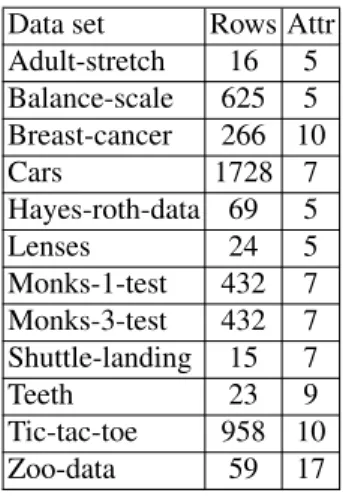
Experiments were made using data sets from UCI Machine Learning Repository [5] and software system Dagger [2]. Some decision tables contain conditional attributes that take unique value for each row. Such attributes were removed. In some tables there were equal rows with, possibly, different decisions. In this case each group of identical
8
rows was replaced with a single row from the group with the most common decision for this group. In some tables there were missing values. Each such value was replaced with the most common value of the corresponding attribute. Prepared 12 data sets were considered as information systems (see Table 1 which contains some information about each of these information systems).
Table 1.Data sets considered as information systems Data set Rows Attr
Adult-stretch 16 5 Balance-scale 625 5 Breast-cancer 266 10 Cars 1728 7 Hayes-roth-data 69 5 Lenses 24 5 Monks-1-test 432 7 Monks-3-test 432 7 Shuttle-landing 15 7 Teeth 23 9 Tic-tac-toe 958 10 Zoo-data 59 17
For each information systemI, we construct the setΦm−v(I)of decision tables
with many-valued decisions and the setΦs−v(I)of decision tables with single-valued
decisions. For each rowrof each tableT ∈Φm−v(I), we apply to this row each of the
considered five greedy heuristics as it was described at the end of the previous section. We rank five heuristics for rowrrelative to the length and coverage of constructed rules and find, for each heuristic, the average ranks relative to length and coverage among all rows of all tables fromΦm−v(I). After that we consider mean of average ranks among
all 12 information systems and obtain overall ranks. Results can be found in Table 2. The best three heuristics for length are M, log, and RM. The best three heuristics for coverage are poly, log, and RM. We study in the same way decision tables with single-valued decisions (see Table 2). The best three heuristics for length are M, RM, and log. The best three heuristics for coverage are poly, log, and RM.
For each heuristic and each rowrof each table T ∈ Φm−v(I), we compare the length of rule constructed by heuristic forr(we denote itlength_greedy) with min-imum length of rule (we denote itlength_min) and calculate the relative difference
length_greedy−length_min
length_min (we assume that
0
0 = 0). The minimum length of rule can be found by dynamic programming algorithms (see [3, 4, 20, 21] for decision tables with single-valued decisions and [11] for decision tables with many-valued decisions). Later, we find average relative difference among all rows of all tables from Φm−v(I), and
overall average relative difference for all 12 information systems. Results can be found in Table 3. The best three heuristics for the length are M (2% difference), RM (4%), and log (13%). Similar study was done for coverage and decision tables with
many-valued decisions. The relative difference is given by coverage_coveragemax−coverage_max _greedy wherecoverage_greedyis the coverage of the rule constructed by greedy heuristic, and coverage_maxis the maximum coverage of the rule calculated by a dynamic program-ming algorithm. The best three heuristics for the coverage are poly (4% difference), log (8%), and maxCov (14%).
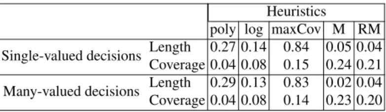
Table 2.Overall ranks for the heuristics Heuristics
poly log maxCov M RM Single-valued decisions Length 3.38 2.25 5.00 2.17 2.21 Coverage 1.67 1.83 4.00 4.21 3.29 Many-valued decisions Length 3.33 2.33 5.00 1.79 2.54 Coverage 1.67 1.83 3.67 4.21 3.62
We study in the same way decision tables with single-valued decisions (see results in Table 3). The best three heuristics for the length are RM (4% difference), M (5%), and log (14%). The best three heuristics for the coverage are poly (4% difference), log (8%), and maxCov (15%).
Table 3.Overall average relative differences for the heuristics Heuristics
poly log maxCov M RM Single-valued decisions Length 0.27 0.14 0.84 0.05 0.04 Coverage 0.04 0.08 0.15 0.24 0.21 Many-valued decisions Length 0.29 0.13 0.83 0.02 0.04 Coverage 0.04 0.08 0.14 0.23 0.20
From the considered results it follows that, for the length minimization, we should use the heuristic M and, probably, the heuristic RM. For the coverage maximization we should use the heuristic poly.
5
Conclusions
We compared five heuristics for construction of association rules in the frameworks of both multi-valued and single-valued decision approaches. We shown that the aver-age relative difference between coveraver-age of rules constructed by the best heuristic and maximum coverage of rules is at most 4%. The same situation is with length. In the future, we are planning to use the best heuristic for coverage in algorithms constructing relatively small systems of rules covering almost all objects in information systems.
10
Acknowledgements
Research reported in this publication was supported by the King Abdullah University of Science and Technology (KAUST).
The authors wish to express their gratitude to anonymous reviewers for useful com-ments.
References
1. Agrawal, R., Imieli´nski, T., Swami, A.: Mining association rules between sets of items in large databases. In: SIGMOD ’93, pp. 207–216. ACM (1993)
2. Alkhalid, A., Amin, T., Chikalov, I., Hussain, S., Moshkov, M., Zielosko, B.: Dagger: A tool for analysis and optimization of decision trees and rules. In: Computational Informatics, So-cial Factors and New Information Technologies: Hypermedia Perspectives and Avant-Garde Experiences in the Era of Communicability Expansion, pp. 29–39. Blue Herons (2011) 3. Amin, T., Chikalov, I., Moshkov, M., Zielosko, B.: Dynamic programming approach for
partial decision rule optimization. Fundam. Inform. 119(3-4), 233–248 (2012)
4. Amin, T., Chikalov, I., Moshkov, M., Zielosko, B.: Dynamic programming approach to opti-mization of approximate decision rules. Inf. Sci. 221, 403–418 (2013)
5. Asuncion, A., Newman, D.J.: UCI Machine Learning Repository (http: //wwwicsuciedu/~mlearn/, 2007),http://www.ics.uci.edu/~mlearn/ 6. Bonates, T., Hammer, P.L., Kogan, A.: Maximum patterns in datasets. Discrete Applied
Mathematics 156(6), 846–861 (2008)
7. Borgelt, C.: Simple algorithms for frequent item set mining. In: Koronacki, J., Ra´s, Z.W., Wierzcho´n, S.T., Kacprzyk, J. (eds.) Advances in Machine Learning II, Studies in Computa-tional Intelligence, vol. 263, pp. 351–369. Springer Berlin Heidelberg (2010)
8. Feige, U.: A threshold oflnnfor approximating set cover. In: Leighton, F.T. (ed.) Journal of the ACM (JACM), vol. 45, pp. 634–652. ACM New York (1998)
9. Han, J., Kamber, M.: Data Mining: Concepts and Techniques. Morgan Kaufmann (2000) 10. Herawan, T., Deris, M.M.: A soft set approach for association rules mining.
Knowledge-Based Systems 24(1), 186–195 (2011)
11. Moshkov, M., Zielosko, B.: Combinatorial Machine Learning - A Rough Set Approach, Studies in Computational Intelligence, vol. 360. Springer (2011)
12. Moshkov, M.J., Piliszczuk, M., Zielosko, B.: Greedy algorithm for construction of partial association rules. Fundam. Inform. 92(3), 259–277 (2009)
13. Moshkov, M.J., Piliszczuk, M., Zielosko, B.: On construction of partial association rules. In: Wen, P., Li, Y., Polkowski, L., Yao, Y., Tsumoto, S., Wang, G. (eds.) RSKT, LNCS, vol. 5589, pp. 176–183. Springer (2009)
14. Nguyen, H.S., ´Sle¸zak, D.: Approximate reducts and association rules - correspondence and complexity results. In: Zhong, N., Skowron, A., Ohsuga, S. (eds.) RSFDGrC, LNCS, vol. 1711, pp. 137–145. Springer (1999)
15. Park, J.S., Chen, M.S., Yu, P.S.: An effective hash based algorithm for mining association rules. In: Carey, M.J., Schneider, D.A. (eds.) SIGMOD Conference, pp. 175–186. ACM Press (1995)
16. Pawlak, Z., Skowron, A.: Rudiments of rough sets. Inf. Sci. 177(1), 3–27 (2007) 17. Rissanen, J.: Modeling by shortest data description. Automatica 14(5), 465–471 (1978) 18. Savasere, A., Omiecinski, E., Navathe, S.B.: An efficient algorithm for mining association
rules in large databases. In: Dayal, U., Gray, P.M.D., Nishio, S. (eds.) VLDB, pp. 432–444. Morgan Kaufmann (1995)
19. Wieczorek, A., Słowi´nski, R.: Generating a set of association and decision rules with statis-tically representative support and anti-support. Information Sciences 277, 56–70 (2014) 20. Zielosko, B.: Sequential optimization ofγ-decision rules. In: Ganzha, M., Maciaszek, L.A.,
Paprzycki, M. (eds.) FedCSIS, pp. 339–346 (2012)
21. Zielosko, B., Chikalov, I., Moshkov, M., Amin, T.: Optimization of decision rules based on dynamic programming approach. In: Faucher, C., Jain, L.C. (eds.) Innovations in Intelligent Machines (4), Studies in Computational Intelligence, vol. 514, pp. 369–392. Springer (2014)
Dynamic Programming Approach for Construction of
Association Rule Systems
Fawaz Alsolami1, Talha Amin1, Igor Chikalov1, Mikhail Moshkov1, and Beata Zielosko2
1 Computer, Electrical and Mathematical Sciences and Engineering Division King Abdullah University of Science and Technology
Thuwal 23955-6900, Saudi Arabia
{fawaz.alsolami, talha.amin, mikhail.moshkov}@kaust.edu.sa [email protected]
2
Institute of Computer Science, University of Silesia 39, Bedzinska St., 41-200 Sosnowiec, Poland
Abstract. In the paper, an application of dynamic programming approach for optimization of association rules from the point of view of knowledge represen-tation is considered. Experimental results present cardinality of the set of asso-ciation rules constructed for information system and lower bound on minimum possible cardinality of rule set based on the information obtained during algo-rithm work.
Key words: association rules, decision rules, dynamic programming, set cover problem, rough sets.
1
Introduction
Association rules are popular form of knowledge representation. They are used in vari-ous areas such as business field for decision making and effective marketing, sequence-pattern in bioinformatics, medical diagnosis, etc. One of the most popular application of association rules is market basket analysis that finds associations between different items that customers place in their shopping baskets.
There are many approaches for mining association rules. The most popular, is Apri-ori algApri-orithm based on frequent itemsets [1]. During years, many new algApri-orithms were designed which are based on, e.g., transaction reduction [2], sampling the data [13], and others [7, 9].
The most popular measures for association rules are support and confidence, how-ever in the literature many other measures have been proposed [8, 9]. In this paper, we are interested in the construction of rules which cover many objects. Maximization of the coverage allows us to discover major patterns in the data, and it is important from the point of view of knowledge representation. Unfortunately, the problem of construction of rules with maximum coverage isN P-hard [6]. The most part of approaches, with the exception of brute-force and Apriori algorithm, cannot guarantee the construction
of rules with the maximum coverage. The proposed dynamic programming approach allows one to construct such rules.
Application of rough sets theory to the construction of rules for knowledge repre-sentation or classification tasks are usually connected with the usage of decision ta-ble [12] as a form of input data representation. In such a tata-ble, one attribute is distin-guished as a decision attribute and it relates to a rule consequence. However, in the last years, associative mechanism of rule construction, where all attributes can occur as premises or consequences of particular rules, is popular. Association rules can be de-fined in many ways. In the paper, a special kind of association rules is studied, i.e., they relate to decision rules. Similar approach was considered in [10, 11], where a greedy algorithm for minimization of length of association rules was studied. In [15], a dy-namic programming approach to optimization of association rules relative to coverage was investigated.
When association rules for information systems are studied and each attribute is sequentially considered as the decision one, inconsistent tables are often obtained, i.e., tables containing equal rows with different decisions. In the paper, two possibilities of removing inconsistency of decision tables are considered. If in some tables there are equal rows with, possibly, different decisions, then (i) each group of identical rows is replaced with a single row from the group with the most common decision for this group, (ii) each group of identical rows is replaced with a single row from the group with the set of decisions attached to rows from the considered group. In the first case, usual decision tables are obtained (decision tables with single-valued decisions) and, for a given row, we should find decision attached to this row. In the second case, decision tables with many-valued decisions are obtained and, for a given row, we should find an arbitrary decision from the set of decisions attached to this row.
For each decision table obtained from the information system, we construct a system of exact rules in the following way: during each step, we choose a rule which covers the maximum number of previously uncovered rows. We stop the construction when all rows of the table are covered. If the obtained system of rules is short enough, then it can be considered as an intelligible representation of the knowledge extracted from the decision table. Otherwise, we can consider approximate rules, and stop the construction of the rule system when the most part of the rows (for example 90% of the rows) are covered.
In [4], the presented algorithm was proposed as application for multi-stage opti-mization of decision rules for decision tables. We extend it to association rules. The presented algorithm can be considered as a simulation of a greedy algorithm for con-struction of partial covers. So we can use lower bound on the minimum cardinality for partial cover based on the information about greedy algorithm work which was obtained in [10].
The paper consists of five sections. Section 2 contains main notions. In Sect. 3, al-gorithm for construction of system of association rule systems is presented. Section 4 contains experimental results for decision tables from UCI Machine Learning Reposi-tory, and Section 5 – short conclusions.
14
2
Main Notions
Aninformation systemIis a rectangular table withn+1columns labeled with attributes f1, . . . , fn+1. Rows of this table are filled by nonnegative integers which are interpreted
as values of attributes.
An association rule forIis a rule of the kind
(fi1 =a1)∧. . .∧(fim =am)→fj=a,
wherefj ∈ {f1, . . . , fn+1},fi1, . . . , fim ∈ {f1, . . . , fn+1} \ {fj}, anda,a1,. . . ,am are nonnegative integers.
The notion of an association rule forI is based on the notions of a decision table and decision rule. We consider two kinds of decision tables: with many-valued decisions and with single-valued decisions.
Adecision table with many-valued decisionsTis a rectangular table withncolumns labeled with (conditional) attributesf1, . . . ,fn. Rows of this table are pairwise different
and are filled by nonnegative integers which are interpreted as values of conditional attributes. Each rowris labeled with a finite nonempty setD(r)of nonnegative integers which are interpreted as decisions (values of a decision attribute). For a given rowrof T, it is necessary to find a decision from the setD(r).
A decision table with single-valued decisions T is a rectangular table with n columns labeled with (conditional) attributes f1, . . . ,fn. Rows of this table are
pair-wise different and are filled by nonnegative integers which are interpreted as values of conditional attributes. Each rowris labeled with a nonnegative integerd(r)which is interpreted as a decision (value of a decision attribute). For a given rowrof T, it is necessary to find the decisiond(r). Decision tables with single-valued decisions can be considered as a special kind of decision tables with many-valued decisions in which D(r) ={d(r)}for each rowr.
For each attributefi ∈ {f1, . . . , fn+1}, the information systemI is transformed into a tableIfi. The columnfiis removed fromIand a table withncolumns labeled with attributesf1, . . . , fi−1, fi+1, . . . , fn+1is obtained. Values of the attribute fi are
attached to the rows of the obtained tableIfias decisions.
The tableIfi can contain equal rows. We transform this table into two decision tables – with many-valued and single-valued decisions. A decision table Ifm−v
i with many-valued decisions is obtained from the tableIfiby replacing each group of equal rows with a single row from the group with the set of decisions attached to all rows from the group. A decision tableIfs−v
i with single-valued decisions is obtained from the tableIfi by replacing each group of equal rows with a single row from the group with the most common decision for this group.
The set{Ifm−v 1 , . . . , I
m−v
fn+1}of decision tables with many-valued decisions obtained from the information systemIis denoted byΦm−v(I). We denote byΦs−v(I)the set
{Ifs−v 1 , . . . , I
s−v
fn+1} of decision tables with single-valued decisions obtained from the information systemI. Since decision tables with single-valued decisions are a special case of decision tables with many-valued decisions, we consider the notion of decision rule for tables with many-valued decisions.
LetT ∈Φm−v(I). For simplicity, letT =Im−v
fn+1. The attributefn+1will be con-sidered as a decision attribute of the tableT. We denote byRow(T)the set of rows of T. LetD(T) =S
r∈Row(T)D(r).
A decision table is calledemptyif it has no rows. The tableT is calleddegenerateif it is empty or has acommondecision, i.e.,T
r∈Row(T)D(r)6=∅. We denote byN(T) the number of rows in the tableT and, for anyt∈ω, we denote byNt(T)the number
of rowsrofT such thatt∈ D(r). Bymcd(T)we denote themost common decision forT which is the minimum decisiont0fromD(T)such thatNt0(T) = max{Nt(T) : t∈D(T)}. IfTis empty thenmcd(T) = 0.
For any conditional attributefi ∈ {f1, . . . , fn}, we denote byE(T, fi)the set of
values of the attribute fi in the table T. We denote by E(T)the set of conditional
attributes for which|E(T, fi)| ≥2.
LetT be a nonempty decision table. AsubtableofT is a table obtained fromT by the removal of some rows. Letfi1, . . . , fim ∈ {f1, . . . , fn}anda1, . . . , am∈ωwhere ωis the set of nonnegative integers. We denote byT(fi1, a1). . .(fim, am)the subtable of the tableT containing the rows fromT which at the intersection with the columns fi1, . . . , fimhave numbersa1, . . . , am, respectively.
As anuncertainty measurefor nonempty decision tables we considerrelative mis-classification errorrme(T) = (N(T)−Nmcd(T)(T))/N(T)whereNmcd(T)(T)is the number of rowsrinT containing the most common decision forT inD(r).
Adecision rule overTis an expression of the kind
(fi1 =a1)∧. . .∧(fim =am)→fn+1=t (1) wherefi1, . . . , fim ∈ {f1, . . . , fn}, anda1, . . . , am, tare numbers fromω. It is possi-ble thatm = 0. For the considered rule, we denoteT0 =T, and ifm >0we denote Tj =T(f
i1, a1). . .(fij, aj)forj = 1, . . . , m. We will say that the decision rule (1) coversthe rowr= (b1, . . . , bn)ofTifrbelongs toTm, i.e.,bi1 =a1, . . . , bim =am. A decision rule (1) overT is called adecision rule forT ift=mcd(Tm), and if m >0, thenTj−1is not degenerate forj = 1, . . . , m, andfij ∈E(T
j−1). We denote byDR(T)the set of decision rules forT.
Let ρ be a decision rule for T which is equal to (1). The value rme(T, ρ) =
rme(Tm) is called the uncertainty of the rule ρ. Let αbe a real number such that
0 ≤ α ≤ 1. We will say that a decision rule ρforT is an α-decision rule for T if rme(T, ρ)≤α. Ifα= 0(in this case, for each rowrcovered byρ, the setD(r) con-tains the decision on the right-hand side ofρ) then we will say thatρis anexactrule. We denote byDRα(T)the set ofα-decision rules forT.
3
Algorithm for Construction of Association Rule System
α-Decision rules for tables from Φm−v(I) can be considered asα-association rules
(modification for many-valued decision model) for the information system I. α-Decision rules for decision tables from Φs−v(I) can be considered asα-association
rules (modification for single-valued decision model) for the information systemI. In this section, we consider an algorithm for construction of an association rule system for
16
I in the frameworks of both many-valued decision model and single-valued decision model. Since decision tables with single-valued decisions are a special kind of deci-sion tables with many-valued decideci-sions, we will discuss mainly many-valued decideci-sion model.
LetT =Ifm−v
n+1. LetSbe a nonempty finite set ofα-decision rules forT (systemof α-decision rules forT), andβbe a real number such that0≤β ≤1. We say thatSis aβ-system ofα-decision rules forT if rules fromScover at least(1−β)N(T)rows ofT.
We describe an algorithmα-β-Rules which, for a decision tableT, and real numbers αandβ,0≤α≤1, and0≤β≤1, constructs aβ-system ofα-decision rules forT. During each step, we choose (based on a dynamic programming algorithm [4]) a deci-sion rule which covers maximum number of uncovered previously rows. We stop when the constructed rules cover at least(1−β)N(T)rows ofT. We denote byRuleα,β(T)
the constructed system of rules.
We denote byC(T, α, β) the minimum cardinality of a β-system ofα-decision rules forT. It is clear thatC(T, α, β)≤ |Ruleα,β(T)|. Using information based on the
work of algorithmα-β-Rules, we can obtain lower bound on the parameterC(T, α, β). During the construction ofβ-system of α-decision rules for T, let the algorithm α-β-Rules selects consequently rules ρ1, . . . , ρt. Let B1, . . . , Bt be sets of rows of T
covered by rulesρ1, . . . , ρt, respectively. SetB0 = ∅,δ0 = 0and, fori = 1, . . . , t,
setδi =|Bi\(B0∪. . .∪Bi−1)|. The information derived from the algorithm’s work consists of the tuple(δ1, . . . , δt)and the numbersN(T)andβ.
From the results obtained in [10] regarding a greedy algorithm for the set cover problem it follows thatC(T, α, β)≥l(T, α, β)where
l(T, α, β)) = max d(1−β)N(T)e −(δ0+. . .+δi) δi+1 :i= 0, . . . , t−1 .
Using algorithm α-β-Rules, for each decision table T ∈ Φm−v(I), we
con-struct the set of rules Ruleα,β(T). As a result, we obtain the system of rules
(α-association rules for the information systemI – modification for many-valued deci-sion model)Rulemα,β−v(I) =S
T∈Φm−v(I)Ruleα,β(T). This system contains, for each
T ∈Φm−v(I), a subsystem which is aβ-system ofα-decision rules forT. We denote
byCm−v(I, α, β)the minimum cardinality of such system. One can show that
Lm−v(I, α, β)≤Cm−v(I, α, β)≤Um−v(I, α, β), Lm−v(I, α, β) =P T∈Φm−v(I)l(T, α, β)andUm−v(I, α, β) = Rule m−v α,β (I) .
We can do the same for the setΦs−v(I)of decision tables with single-valued
deci-sions. As a result, we obtain the system of rules (α-association rules for the information systemI– modification for single-valued decision model)Rulesα,β−v(I) =S
T∈Φs−v(I) Ruleα,β(T)which contains, for eachT∈Φs−v(I), a subsystem which is aβ-system of
α-decision rules forT. DenoteCs−v(I, α, β)the minimum cardinality of such system.
One can show that
Table 1.Total number of rules (upper bound / lower bound) Ls−v(I, α, β) =P T∈Φs−v(I)l(T, α, β)andUs−v(I, α, β) = Rule s−v α,β(I) .
4
Experimental Results
Experiments were made using data sets from UCI Machine Learning Repository [5] and software system Dagger [3]. Some decision tables contain conditional attributes that take unique value for each row. Such attributes were removed. In some tables, there were equal rows with, possibly, different decisions. In this case each group of identical rows was replaced with a single row from the group with the most common decision for this group. In some tables there were missing values. Each such value was replaced with the most common value of the corresponding attribute.
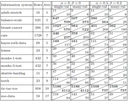
Prepared 12 data sets were considered as information systems. Table 1 contains name (column “Information system”), number of rows (column “Rows”), and number of attributes (column “Attr”) for each of the considered information systems. Table 1 presents also upper / lower bounds (see descriptions at the end of the previous section) onCm−v(I, α, β)(column “many-val”) and onCs−v(I, α, β)(column “single-val”)
for pairs (α= 0,β= 0) and (α= 0.3,β = 0.2).
We can see that, for tables with many-valued decisions, upper and lower bounds on the number of rules are less than or equal to the bounds for decision tables with single-valued decision. We considered a threshold
18
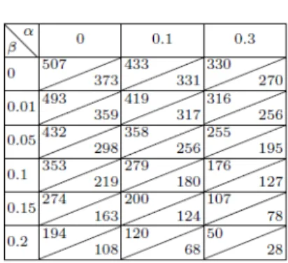
Table 2.Total number of rules for information system balance-scale with 5 attributes
as a reasonable upper bound on the number of rules if a system of rules is used for knowledge representation. In the case α = 0andβ = 0, the threshold is exceeded for five information systems (see numbers in bold): balance-scale, breast-cancer, cars, hayes-roth-data, and tic-tac-toe. The consideration of approximate rules and partial cov-ers can improve the situation. In the caseα = 0.3andβ = 0.2, the threshold is ex-ceeded for three information systems (balance-scale, breast-cancer, and tic-tac-toe) if we consider decision tables with single-valued decisions and for two information sys-tems (breast-cancer and tic-tac-toe) if we consider decision tables with many-valued decisons.
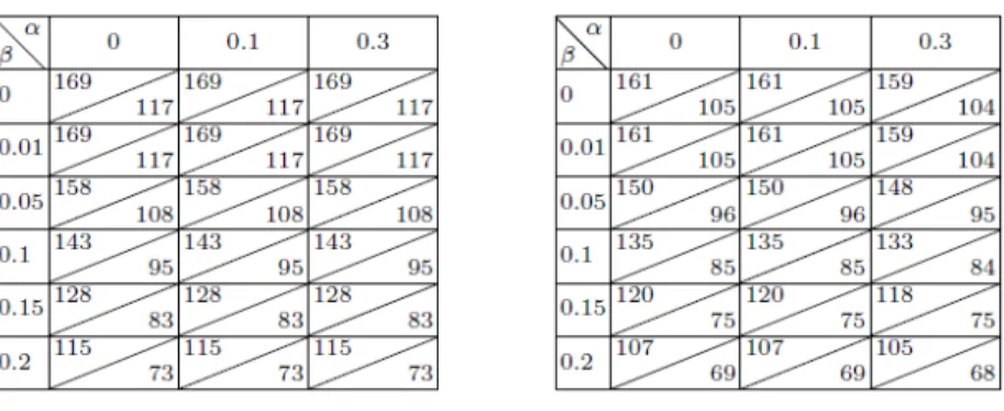
For four information systems (balance-scale, breast-cancer, cars, and hayes-roth-data), upper / lower bounds on Cm−v(I, α, β)) and on Cs−v(I, α, β)) for β ∈
{0,0.01,0.05,0.1,0.15,0.2}andα∈ {0,0.1,0.3}can be found in Tables 2, 3, 4, and 5.
5
Conclusions
In the paper, an algorithm for construction of association rule system is proposed. It sim-ulates the work of greedy algorithm for set cover problem. Experimental results present cardinality of the set of association rules constructed for information system and lower bound on minimum possible cardinality of such set based on the information about the algorithm work. In the future, the length of constructed association rules will be stud-ied also. We are planning to extend an approach proposed in [14] for decision rules to construction of association rule systems. This approach allows one to construct rules with coverage close to maximum and requires less time than the dynamic programming approach.
Table 3.Total number of rules for information system breast-cancer with 10 attributes
20
Table 5.Total number of rules for information system hayes-roth-data with 5 attributes
Acknowledgements
Research reported in this publication was supported by the King Abdullah University of Science and Technology (KAUST).
The authors wish to express their gratitude to anonymous reviewers for useful com-ments.
References
1. Agrawal, R., Imieli´nski, T., Swami, A.: Mining association rules between sets of items in large databases. In: SIGMOD ’93, pp. 207–216. ACM (1993)
2. Agrawal, R., Srikant, R.: Fast algorithms for mining association rules in large databases. In: Bocca, J.B., Jarke, M., Zaniolo, C. (eds.) VLDB, pp. 487–499. Morgan Kaufmann (1994) 3. Alkhalid, A., Amin, T., Chikalov, I., Hussain, S., Moshkov, M., Zielosko, B.: Dagger: A tool
for analysis and optimization of decision trees and rules. In: Computational Informatics, So-cial Factors and New Information Technologies: Hypermedia Perspectives and Avant-Garde Experiences in the Era of Communicability Expansion, pp. 29–39. Blue Herons (2011) 4. Alsolami, F., Amin, T., Chikalov, I., Moshkov, M.: Multi-stage optimization of decision rules
for knowledge discovery and representation. Knowledge and Information Systems (2015), (submitted)
5. Asuncion, A., Newman, D.J.: UCI Machine Learning Repository (http: //wwwicsuciedu/~mlearn/, 2007),http://www.ics.uci.edu/~mlearn/ 6. Bonates, T., Hammer, P.L., Kogan, A.: Maximum patterns in datasets. Discrete Applied
Mathematics 156(6), 846–861 (2008)
7. Borgelt, C.: Simple algorithms for frequent item set mining. In: Koronacki, J., Ra´s, Z.W., Wierzcho´n, S.T., Kacprzyk, J. (eds.) Advances in Machine Learning II, Studies in Computa-tional Intelligence, vol. 263, pp. 351–369. Springer Berlin Heidelberg (2010)
8. Glass, D.H.: Confirmation measures of association rule interestingness. Knowledge-Based Systems 44(0), 65–77 (2013)
9. Han, J., Kamber, M.: Data Mining: Concepts and Techniques. Morgan Kaufmann (2000) 10. Moshkov, M.J., Piliszczuk, M., Zielosko, B.: Greedy algorithm for construction of partial
11. Moshkov, M.J., Piliszczuk, M., Zielosko, B.: On construction of partial association rules. In: Wen, P., Li, Y., Polkowski, L., Yao, Y., Tsumoto, S., Wang, G. (eds.) RSKT, LNCS, vol. 5589, pp. 176–183. Springer (2009)
12. Pawlak, Z., Skowron, A.: Rudiments of rough sets. Inf. Sci. 177(1), 3–27 (2007)
13. Toivonen, H.: Sampling large databases for association rules. In: Vijayaraman, T.M., Buch-mann, A.P., Mohan, C., Sarda, N.L. (eds.) VLDB, pp. 134–145. Morgan Kaufmann (1996) 14. Zielosko, B.: Optimization of approximate decision rules relative to coverage. In: Kozielski,
S., Mrózek, D., Kasprowski, P., Małysiak-Mrózek, B., Kostrzewa, D. (eds.) BDAS 2014. LNCS, vol. 8537, pp. 170–179. Springer (2014)
15. Zielosko, B.: Global optimization of exact association rules relative to coverage. In: Kryszkiewicz, M., Bandyopadhyay, S., Rybi´nski, H., Pal, S.K. (eds.) PReMI 2015. LNCS, vol. 9124, pp. 428–437. Springer (2015)
Considering Concurrency in Early Spacecraft Design
Studies
Jafar Akhundov, Peter Tröger, and Matthias Werner Operating Systems Group, TU Chemnitz, Germany
{jafar.akhundov,peter.troeger,matthias.werner}@cs.tu-chemnitz.de
Abstract. In real-world spacecraft systems, concurrent system activities must be constrained for energy efficiency and functional reasons. Such constraints must be considered in the early design phases, in order to avoid costly reiterations and modifications of the proposed system design in later phases. Although some ini-tial attempts for using formal specifications exist in the domain, there is a lack of concurrency support in the utilized approaches. In this paper, we therefore first formalize an existing domain-specific language for specifying spacecraft designs and their constraints. Since this language does not support the modelling of con-currency issues, we extend it accordingly and map it to standard timed automata, based on a general system model. The new-style specifications can now be pro-cessed with existing and proven automata modelling tools, which enables faster and more reliable feasibility checks for early spacecraft system designs.
1
Introduction
The model-based engineering paradigm is widely accepted in the aerospace industry. One specific implementation is "Concurrent Engineering (CE)", an approach that has evolved into an important support mechanism for early space mission design decisions. It is supposed to clarify the baseline requirements and design properties for a future spacecraft, such as overall mass, power consumption and costs for development and operation. Studies have shown that up to 85% of the overall spacecraft project costs result from decisions made in this early phase [14].
During the CE project phase, multiple spacecraft design alternatives are simultane-ously created, refined and analyzed by a group of engineers. Everybody in this group has an own range of responsibilities, such as the consideration of satellite trajectories, the realization of communication mechanisms, or the consideration of thermal aspects [11]. This makes the evaluation and ranking of architecture variations a complicated issue, since local design changes always have implications on global system scope. Those modifications may even impact the feasibility of the complete system design, if not correctly tracked and understood before the next project phase. This led to the development of feasibility checking approaches as part of CE in the past. They are con-ducted iteratively after each major design change, to provide feedback for engineers and the spacecraft customer.
The following paper discusses the consideration of concurrency demands and re-strictions in the CE project phase based on a formal specification. Section 2 first intro-duces an abstract system model for spacecraft systems, in order to restrict the model
entities to a necessary minimum. Section 3 then explains a domain-specific language being used in a German spacecraft project for the formulation of constraints and prop-erties. In Section 4, we show how this DSL must be enhanced to consider concurrency issues properly. Section 5 finally explains how the resulting DSL can be translated to timed automata for better analysis support from existing tools.
2
Spacecraft System Model
A spacecraft system can be modeled as a set of internal and external state variables S=IS∪ES. The internal statesiis defined by all state variables that can be directly manipulated through spacecraft’s activities, e.g., the charging level of the battery or the available free memory. External state variables change by themselves and are not directly affected by spacecraft activities. Examples are temperature, the time, or the availability of sun light. They constitute the external statese.
The spacecraft activity can be abstractly defined based on the idea of interacting components. One relevant property here is the consideration of their concurrent activ-ities and their relation to time. Let T = {τ1, ..., τn}, n ∈ Nbe a set of operational states representing activities of the spacecraft components, e.g. the active charging of the satellite battery from solar panels or the usage of some data transmission down-link. I.e., for eachτi, there exists a transition functionfi(se, si, ∆t) = ∆sithat describes
the change of the internal system’s state if a component is active for the time∆t. In real-world satellite systems, concurrent component activities must be constrained for energy efficiency and functional reasons. Not all spacecraft components can be ac-tive at the same time. LetC = {c1, ..., ck}, k ∈ Nrepresent a set of constraints for the state variables. Please note that the mission goals can be seen as special mission constraints.
Given the above definitions, ascheduleor a planis defined as a mapping of the component activity setT onto a set of time intervals:
P :T 7→ I, (1)
whereI ={(b, f) :b, f ∈R+, b < f}is a set of finite length time intervals with b, f begin the start- and end-times of the intervals, respectively. As a side condition, all Cimust be true at any time.
Based on the given system model, we are now discussing how constraints can be formulated and checked for a specific system model instance.
3
DSL-Based Constraint Description
Different methods can be used to check a spacecraft system model’s compliance with the intended constraints and goals for the planned mission time. Schaus et al. described how an expert can formulate such requirements in a dedicateddomain specific language (DSL)and use search algorithms to check the feasibility with respect to the given con-straints [10]. The proposed syntax was used to create a description for a representative flying mission called satellite TET-1 [7, 16]. The DSL syntax turned out to be detailed
24
enough to be fed into a search algorithm that looks for an execution trace fulfilling all conditions as mission plan [12].
Originally, the proposed concept was calledcontinuous verification. We avoid the term ‘verification’ intentionally here, since at such an early design phase there is no real detailed system specification against which the system would be formally verified. Actually, creating unambiguous specifications is the purpose of the whole preliminary analysis. Instead of ‘verification’, the terms ‘feasibility study/check’ will be used.
In the published DSL syntax, the engineer can define different system components being exclusively active (calledstates) and system parameters (calledoperational state variables) which can be changed by the components’ activities. The values of these parameters define the global system state. I.e., there exist implicit constraints
∀i, j, i6=j, τi⇒ ¬τj (2)
The mission goal is defined as a constraint on the operational state variables. Addi-tional constraints beside the central mission goal can also be formulated. Furthermore, for every component there are corresponding rates of changes to the system parameters. The generated mission plan is a chain of activity periods derived from this description, such asBattery Charge→Collect Data with Cameras→Send Data to Earth→Idle
→....
Since satellite systems depend not only on the internal components, but also on the execution environment, there is a possibility to describe such environmental properties in the DSL, too. This is done by parameterizing external simulation models (SGP4) [10, 6] to compute satellite trajectories and generate periodic external events that activate components.
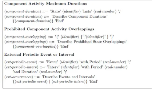
The original DSL from [10] is translated to the grammar description in Figure 1. It contains of the following parts:
– Thesolverconstruct determines the actual search algorithm which is used to find an appropriate solution.
– Thestate parameterstogether with theinitial parameter valuesdefine system pa-rameters which determine spacecraft system’s state.
– Theoperational statesrepresent the components of the satellite being active. – Thestarting statedefines the first component being active.
– Theoperational state changesdefine rates of change of system parameters by com-ponents’ activities.
– For some of the state parameters, there could exist upper or lower bounds that are determined in theoperational constraintsconstruct.
– The goal of the whole mission can be defined as a set of state parameter values which can be set in theoperational goalssection.
– External events and intervals are determined by using externalsimulation modules being defined. Only the construct for a simulation step is given, since the rest is initialization of the satellite’s trajectory and coordinates of the ground stations for down-link and up-link communications.
Since in the original language there is no component concurrency being considered, only one component resp. operational state can be active at any point in time. Con-sequently, there is no explicit time notion in the language, with the only exception of
Fig. 1.Syntactical structure of an existing domain-specific language for spacecraft de-sign descriptions, derived from [10]. Some non-terminals, such as identifiers, are omit-ted due to space restrictions.
26
simulation step which is the parameter fed to the external orbit simulator. This also de-termines the values for the changes of state parameters and the maximum number of steps before the mission deadline.
An important issue in the aforementioned DSL is that the operational state of the system, a vector of all state variables, is assumed to be directly bounded to thestate of the currently active component. In other words: The system is specified with having only one active component at a time. This is an obvious over-constraining of the model, since a satellite as a system cannot be observed isolated from its environment. Concur-rency consideration should be therefore not only a possible, but a desirable property. Several components of a satellite can be active simultaneously. One simple example is data being sent to earth while the battery is being charged. Furthermore, such a restric-tive execution model can lead to the false negarestric-tive check result, although the mission could still be possible to execute with a more “dense” plan1.
Supporting concurrency in the DSL and the implied execution model would lead to increased expressiveness of the language and allow for more realistic derivable analysis results. Furthermore, with the concurrent execution model the generated plans are more ‘dense’ and thus the probability of a false negative result of the feasibility checking is lower.
4
Extended DSL Syntax
Given the formal system model from Section 2, we translate the semantics of the given DSL first into the set-theoretical constructs to understand the missing expressivity and determine the necessary enhancements:
– Asolveris implementation-specific and defines a search method to trace the state space of a given problem. Hence, it is not part of the formal model.
– Thestate parametersare represented by the setSof state variables in the formal model. Their initial values are implementation-specific.
– Theoperational statesare defined by the setT of the formal model. Starting State does not need to be determined by the engineer since a satellite can have several active components simultaneously and their enabling depends on the validity con-ditions.
– Theoperational state changesare also defined by the setT of the formal model. – Theoperational goals and constraintsare represented by the setC of the formal
model.
There is no explicit notion of duration in the given DSL. The set of prohibited over-lapped component activities is also missing in the explicit form. Implicitly, however, one could say that the set is given by the assumption in the execution model that all over-lapped executions are forbidden. Furthermore, events which enable certain component activities are not explicitly present in the DSL. They are generated by the simulation modules and directly fed to the search algorithm.
1
Here, the term “plan density” is loosely coined to describe a possibility to use overlapping time intervals to pack more activity into the mission time.
For supporting the missing concurrency semantics, the DSL is now enhanced with three syntactical constructs, as shown in Figure 2: Explicit durations per component activity, prohibited component activity overlapping, and events + durations.
Fig. 2.DSL Enhancements for Concurrency Support
As a result of the reformulation and enhancement of the DSL grammar, the problem of feasibility analysis can now be reformulated as an off-line scheduling problem with several constraints [8]. Therefore, any formal modeling method supporting concurrency and having explicit notion of time would be a potential solution helper for the problem. Well-known examples are Timed CSP, Timed Petri Nets, Timed Automata, or Hybrid Automata.
We decided to map the enhanced DSL to Timed Automata [1, 2] for several reasons:
– The concepts of timed automata are easier accepted by engineers unrelated to com-putational logic and formal modeling.
– The structure of the DSL introduced in [10] translates one-to-one to a automata description.
– Timed automata have been proven to be more expressive than Timed Petri Nets [5] and just as expressive as Timed CSP models[9]
Although hybrid automata are more general and more expressive than timed au-tomata [13], we sticked with pure time auau-tomata eventually, since they provide enough modeling capabilities for the given concurrency analysis problem.

![Fig. 1. Syntactical structure of an existing domain-specific language for spacecraft de- de-sign descriptions, derived from [10]](https://thumb-us.123doks.com/thumbv2/123dok_us/1937971.2785850/33.918.239.685.142.876/syntactical-structure-existing-specific-language-spacecraft-descriptions-derived.webp)