PAC-Bayes Unexpected Bernstein Inequality

arXiv:1905.13367v2 [cs.LG] 3 Nov 2019

PAC-Bayes Un-Expected Bernstein Inequality

Zakaria Mhammedi

The Australian National University and Data61

[email protected]

Peter D. Grünwald CWI and Leiden University

[email protected]

Benjamin Guedj

Inria and University College London

[email protected]

Abstract

We present a new PAC-Bayesian generalization bound. Standard bounds contain a√Ln⋅KL/ncomplexity term which dominates unlessLn, the empirical error of the learning algorithm’s randomized predictions, vanishes. We manage to re-placeLnby a term which vanishes in many more situations, essentially whenever the employed learning algorithm is sufficiently stable on the dataset at hand. Our new bound consistently beats state-of-the-art bounds both on a toy example and on UCI datasets (with large enoughn). Theoretically, unlike existing bounds, our new bound can be expected to converge to0faster whenever a Bernstein/Tsybakov condition holds, thus connecting PAC-Bayesian generalization and excess risk

bounds—for the latter it has long been known that faster convergence can be ob-tained under Bernstein conditions. Our main technical tool is a new concentration inequality which is like Bernstein’s but withX2

taken outside its expectation.

1

Introduction

PAC-Bayesian generalization bounds [1,7,8,16,17,19,27,28,29] have recently obtained renewed interest within the context of deep neural networks [13,33,41]. In particular, Zhou et al. [41] and Dziugaite and Roy [13] showed that, by extending an idea due to Langford and Caruana [22], one can obtain nontrivial (but still not very strong) generalization bounds on real-world datasets such as MNIST and ImageNet. Since using alternative methods, nontrivial generalization bounds are even harder to get, there remains a strong interest in improved PAC-Bayesian bounds. In this paper, we provide a considerably improved bound whenever the employed learning algorithm is sufficiently

stableon the given data.

Most standard bounds have an order√Ln⋅COMPn/nterm on the right, whereCOMPnrepresents model complexity in the form of a Kullback-Leibler divergence between a prior and a posterior, andLn is theposterior expected losson the training sample. The latter only vanishes if there is a sufficiently large neighborhood around the “center” of the posterior at which the training error is 0. In the two papers [13,41] mentioned above, this is not the case. For example, the various deep net experiments reported by Dziugaite et al. [13, Table 1] withn=150000all haveLnaround0.03, so that√COMP_n/nis multiplied by a non-negligible√0.03≈0.17. Furthermore, they haveCOMPn increasing substantially withn, making√Ln⋅COMPn/nconverge to0at rate slower than1/√n. In this paper, we provide a bound (Theorem3) withLnreplaced by a second-order termVn—a term which will go to0in many cases in whichLn does not. This can be viewed as an extension of an earlier second-order approach by Tolstikhin and Seldin [38] (TS from now on); they also replaceLn,

as they write, in classification settings (our primary interest), their replacement is not much smaller thanLnitself. Instead ourVn can be very close to0in classification even whenLnis large. While the TS bound is based on an “empirical” Bernstein inequality due to [26]1_{, our bound is based on}

a different modification of Bernstein’s moment inequality in which the occurrence ofX2

is taken outside of its expectation (see Lemma13). We note that an empirical Bernstein inequality was introduced in [3, Theorem 1], and the name “Empirical Bernstein” was coined in [31].

The termVnin our bound goes to0—and our bound improves on existing bounds—whenever the employed learning algorithm is relatively stable on the given data; for example, if the predictor learned on an initial segment (say,50%) of the dataset performs similarly (i.e.assigns similar losses

to the same samples) to the predictor based on the full data. This improvement is reflected in our experiments where, except for very small sample sizes, we consistently outperform existing bounds both on a toy classification problem with label noise and on standard UCI datasets [12]. Of course, the importance of stability for generalization has been recognized before in landmark papers such as [6,32,37], and recently also in the context of PAC-Bayes bounds [34]. However, the data-dependent stability notion “Vn” occurring in our bound seems very different from any of the notions discussed in those papers.

Theoretically, a further contribution is that we connect our PAC-Bayesian generalization bound to

excess risk bounds; we show that (Theorem7) our generalization bound can be of comparable size to

excess risk bounds up to an irreduciblecomplexity-freeterm that is independent of model complexity.

The excess risk bound that can be attained for any given problem depends both on the complexity of the set of predictorsHand on the inherent “easiness” of the problem. The latter is often measured in terms of the exponentβ ∈ [0,1]of the Bernstein conditionthat holds for the given problem

[5, 14,18], which generalizes the exponent in the celebratedTsybakov margin condition [4,39].

The largerβ, the faster the excess risk converges. In Section5, we essentially show that the rate at

which the√Vn⋅COMPn/nterm goes to0can also be bounded by a quantity that gets smaller asβ gets larger. In contrast, previous PAC-Bayesian bounds do not have such a property.

Contents. In Section2, we introduce the problem setting and provide a first, simplified version of our main theorem. Section3gives our main bound. Experiments are presented in Section4, followed by theoretical motivation in Section5. The proof of our main bound is provided in Section6, where we first present the convenient ESI language for expressing stochastic inequalities, and (our main tool) the unexpected Bernstein lemma (Lemma13). The paper ends with an outlook for future work.

2

Problem Setting, Background, and Simplified Version of Our Bound

LetHbe a hypothesis set and ℓ ∶ H×Z → [0, b], b > 0, be a bounded loss function such that

ℓh(Z)∶=ℓ(h, Z)denotes the loss that hypothesishmakes onZ. We call any such tuple(D, ℓ,H) alearning problem. For a given hypothesish∈ H, we denote itsrisk(expected loss on a test sample

of size 1) byL(h)∶=E_Z∼D[_ℓh(_Z)]and its empirical error by_Ln(_h)_∶= 1 n∑

n

i=1ℓh(Zi). For any distributionP onH, we writeL(P)∶=E_h∼P[L(h)]andLn(P)∶=Eh∼P[Ln(h)].

For anym∈[n]and any variablesZ1, . . . , Z_ninZ, we denoteZ_≤m∶=(Z1, . . . , Z_m)andZ_<m∶=

Z_≤m−1, with the convention thatZ_≤0 =∅. Similarly, we denoteZ_≥m∶=(Zm, . . . , Zn)andZ>m∶=

Z_≥m+1, with the convention thatZ_≥n+1 =∅. As is customary in PAC-Bayesian works, alearning

algorithmis a (computable) functionP ∶⋃n

i=1Zi → P(H)that, upon observing inputZ_≤n ∈ Zn, outputs a “posterior” distributionP(Z_≤n)(⋅)onH. The posterior could be a Gibbs or a generalized-Bayesian posterior but also other algorithms. When no confusion can arise, we will abbreviate

P(Z_≤n)toPn, and denote P0 any “prior” distribution, i.e. a distribution onHwhich has to be

specified in advance, before seeing the data; we will use the conventionP(_∅)=P0. Finally, we

denote the Kullback-Leibler divergence betweenPnandP0by KL(P_n∥P0).

Comparing Bounds.Both existing state-of-the-art PAC-Bayes bounds and ours essentially take the following form; there exists constantsP,A,C≥ 0, and a functionεδ,n, logarithmic in 1/δandn, 1_{An alternative form of empirical Bernstein inequality appears in [40], based on an inequality due to [10].}

such that for allδ∈]0,1[, with probability at least1₋δover the sampleZ1, . . . , Zn, it holds that, L(Pn)−Ln(Pn)≤P⋅ √ Rn⋅(COMPn+εδ,n) n +A⋅ COMPn+εδ,n n +C⋅ √ R′ n⋅εδ,n n , (1)

whereRn, R′n ≥ 0 are sample-dependent quantities which may differ from one bound to another. Existing classical bounds that after slight relaxations take on this form are due to Langford and Seeger [23,36], Catoni [9], Maurer [25], and Tolstikhin and Seldin (TS) [38] (see the latter for a nice overview). In all these cases, COMP_n = KL(Pn∥P0), R′_n = 0, and—except for the TS

bound—Rn=Ln(Pn). For the TS bound,Rnis equal to the empirical loss variance. Our bound in Theorem3also fits (1) (after a relaxation), but with considerably different choices forCOMPn,R′_n,

andRn.

Of special relevance in our experiments is the bound due to Maurer [25], which as noted by TS [38] tightens the PAC-Bayes-kl inequality due to Seeger [35], and is one of the tightest known generalization bounds in the literature. It can be stated as follows: forδ ∈]0,1[,n ≥ 8, and any

learning algorithmP, with probability at least1₋δ,

kl(L(Pn), Ln(Pn))≤

KL₍Pn∥P0)+ln 2√_n

δ

n , (2)

whereklis the binary Kullback-Leibler divergence. Applying the inequalityp≤q₊√2qkl(p∥q)₊

2 kl(p∥q)to (2) yields a bound of the form (1) (see [38] for more details). Note also that using Pinsker’s inequality together with (2) implies McAllester’s classical PAC-Bayesian bound [27]. We now present a simplified version of our bound in Theorem3below as a corollary.

Corollary 1. For any1≤m<nand any deterministic estimatorˆh∶⋃n

i=1Zi→H(such asERM),

there existsP_,A_,C>0, such that(1)holds with probability at least1₋δ, with

COMP_n=KL(Pn∥P(Z≤m))+KL(Pn∥P(Z>m)), (3) R′_n∶=V_n′∶= 1 n m ∑ i=1 ℓˆ_h(Z >m)(Zi) 2 + 1 n n ∑ j=m+1 ℓˆ_h(Z ≤m)(Zj) 2 , (4) Rn∶=Vn∶= 1 nEh∼Pn ⎡⎢ ⎢⎢ ⎣ m ∑ i=1 (ℓh(Zi)−ℓˆ_h (Z>m)(Zi)) 2 + n ∑ j=m+1 (ℓh(Zj)−ℓˆ_h (Z≤m)(Zj)) 2⎤⎥ ⎥⎥ ⎦. (5)

Like in TS’s and Catoni’s bound, but unlike McAllester’s and Maurer’s, ourεδ,ngrows as(ln lnn)/δ. Another difference is that our complexity term is a sum of two KL divergences, in which the prior (in this case P(Z_≤m)orP(Z>m)) is “informed”—whenm=n/2, it is really the posterior based on half the sample. Our experiments confirm that this tends to be much smaller than KL₍Pn∥P0).

Other bounds can also be modified to make use of informed priors and replace the KL(Pn∥P0)term

byCOMPnin (3). This is formalized in the next section.

A larger difference between our bound and others is in the fact that we have Rn =Vn instead of the typical empirical errorRn = Ln(Pn). Only TS [38] have aRn that is somewhat reminiscent of ours; in their caseRn=Eh∼Pn[∑ni=1(ℓh(Zi)−Ln(h))

2

]/(n−1)is the empirical loss variance. The crucial difference to ourVn is that the empirical loss variance cannot be close to0 unless a sizeablePn-posterior region ofhhas empirical error almost constant on most data instances. For classification with 0-1 loss, this is a strong condition since the empirical loss variance is equal to

nLn(Pn)(1−Ln(Pn))/(n−1), which is only close to0if Ln(Pn)is itself close to 0or1. In contrast, ourVn can go to zero0 even if the empirical error and variance do not, as long as the learning algorithm is sufficiently stable. This can be witnessed in our experiments in Section4. In Section5, we argue more formally that under a Bernstein condition, the√Vn⋅COMPn/nterm in our bound can be much smaller than√COMPn/n. Note, finally, that the termVn has a two-fold cross-validation flavor, but in contrast to a cross-validation error, forVnto be small, it is sufficient that the losses aresimilar, not that they are small.

The price we pay for havingRn=Vnin our bound is the right-most, irreducible remainder term in (1) of order at mostb/√n. Note, however, that this term is decoupled from the complexityCOMPn,

and thus it is not affected byCOMPn growing with the “size” ofH. The following lemma gives a tighter bound (tighter than theb/√njust mentioned) on the irreducible term:

Lemma 2. Suppose that the loss is bounded by 1 (i.e. b=1) and thatnis even, and letm=n/2. Forδ∈]0,1[,R_n′ as in(4), and any estimatorhˆ ∶⋃n

i=1Zi→H, we have, with probability at least

1−δ, √ R′ n n ≤ √ 2(L(ˆh(Z_>m))+L(ˆh(Z≤m))) n + 4√ln4 δ n . (6)

Behind the proof of the lemma is an application of Hoeffding’s and the empirical Bernstein inequal-ity [26] (see SectionC). Note that in the realizable setting, the first term on the RHS of (6) can be of orderO(1/n)with the right choice of estimatorˆh(e.g. ERM). In this case (still in the

realiz-able setting), our irreducible term would go to zero at the same rate as other bounds which have

Rn=Ln(Pn).

3

Main Bound

We now present our main result in its most general form. Letϑ(η) ∶= (−ln(1₋η)₋η)/η2

and

cη∶=η⋅ϑ(ηb), forη∈]0,1/b[, whereb>0is an upper-bound on the lossℓ.

Theorem 3. [Main Theorem]Let Z1, . . . , Z_n be i.i.d. withZ1 ∼ D. Letm ∈ [0..n]andπbe

any distribution with support on a finite or countable gridG ⊂]0,1/b[. For anyδ∈]0,1[, and any learning algorithmsP, Q∶⋃n i=1Zi→P(H), we have, L(Pn)≤Ln(Pn)+inf η∈G ⎧⎪⎪ ⎨⎪⎪ ⎩cη⋅Vn+ COMP_n+2 ln 1 δ⋅π(η) η_⋅n ⎫⎪⎪ ⎬⎪⎪ ⎭+νinf∈G ⎧⎪⎪ ⎨⎪⎪ ⎩cν⋅V ′ n+ ln 1 δ⋅π(ν) ν_⋅n ⎫⎪⎪ ⎬⎪⎪ ⎭, (7) with probability at least1₋δ, whereCOMPn,Vn′, andVnare the random variables defined by:

COMPn∶=KL(Pn∥P(Z≤m))+KL(Pn∥P(Z>m)), (8) V′ n∶= 1 n m ∑ i=1 E_h∼Q(Z >i)[ℓh(Zi) 2 ]+ 1 n n ∑ j=m+1 E_h∼Q(Z <j)[ℓh(Zj) 2 ], Vn∶= 1 nEh∼Pn ⎡⎢ ⎢⎢ ⎣ m ∑ i=1 (ℓh(Zi)−Eh′_∼Q(Z>i)[ℓ_h′(Z_i)]) 2 + n ∑ j=m+1 (ℓh(Zj)−Eh′_∼Q(Z<j)[ℓ_h′(Z_j)]) 2⎤⎥ ⎥⎥ ⎦.

While the result holds for all0 ≤m≤n, in the remainder of this paper, we assume for simplicity

thatnis even and thatm=n/2. We will also be using the gridGand distributionπdefined by

G∶={1 2_b, . . . , 1 2K_b∶K∶=⌈log2( 1 2 √ _n ln1 δ)⌉}

, and π≡uniform distribution overG. (9) Roughly speaking, this choice of _G ensures that the infima inη andν in (7) are attained within [minG,maxG]. Using the relaxation cη ≤ η/2+η

2

11b/20, forη ≤ 1/(2b), in (7) and tuningη

andν within the gridGdefined in (9) leads to a bound of the form (1). Furthermore, we see that

the expression ofVn in Corollary1now follows whenQis chosen such that, for1≤i≤m<j ≤

n,Q(Z_>i) ≡ δ(hˆ(Z_>m)) andQ(Z_<j) ≡ δ(hˆ(Z_≤m)), for some deterministic estimator_hˆ_{, where}

δ(h)(⋅)denotes the Dirac distribution ath∈H.

Online Estimators. It is clear that Theorem 3 is considerably more general than its Corollary

1; when predicting thej-th point Zj, j > m, in the RHS sum ofVn, we could use a posterior

Q(Z_<j)≡ δ(hˆ(Z<j))which does not only depend onZ1, . . . , Zm, but also on part of the second

sample, namelyZm+1, . . . , Z_j−1, and analogously when predictingZi,i≤ m, in the LHS sum of

Vn. We can thus base our bound on a sum of errors achieved byonline estimators(ˆh(Z_<j))and

(ˆ_h(Z

>i))which converge to the finalˆh(Z≤n)based on the full data. Doing this would likely improve our bounds, but we did not try it in our experiments since it is computationally demanding.

Informed Priors. Other bounds can also be modified to make use of “informed priors” from each half of the data; in this case, the KL(Pn∥P0)term in these bounds can be replaced byCOMP_ndefined

in (8). As revealed by additional experiments in the AppendixH, doing this substantially improves the corresponding bounds when the learning algorithm is sufficiently stable. Here we show how this can be done for Maurer’s bound in (2) (the details for other bounds are postponed to AppendixA).

Lemma 4. Letδ∈]0,1[andm∈[0..n]. In the setting of Theorem3, we have, with probability at least1₋δ, kl(L(Pn), Ln(Pn))≤ KL(Pn∥P(Z≤m))+KL(Pn∥P(Z>m))+ln 4√_m(n−_m) δ n . (10)

Remark 5. (Useful for Section5below) Though this may deteriorate the bound in practice, Theo-rem3allows choosing a learning algorithmPsuch that for1≤m<n,P(Z_≤m)≡P(Z_>m)≡P0

(i.e.no informed priors); this results inCOMPn=2KL(Pn∥P0)—the bound is otherwise unchanged.

Biasing. The termVnin our bound can be seen as the result of “biasing” the loss when evaluating the generalization error on each half of the sample. The TS bound, having a second order variance term, can be used in a way as to arrive at a bound like ours with the same Vn as in Corollary1. The idea here is to apply the TS bound twice (once on each half of the sample) to the biased losses

ℓ(h,⋅)−ℓ(hˆ(Z_≤m),⋅)andℓ(h,⋅)−ℓ(ˆh(Z>m),⋅), then combine the results with a union bound. The details of this are postponed to AppendixB. Note however, that this trick will not lead to a bound with aVnterm as in Theorem3,i.e. with the online posteriors(Q(Z>i))and(Q(Z<j))which get closer and closer to the finalQ(Z_≤m)based on the full sample.

4

Experiments

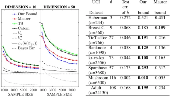
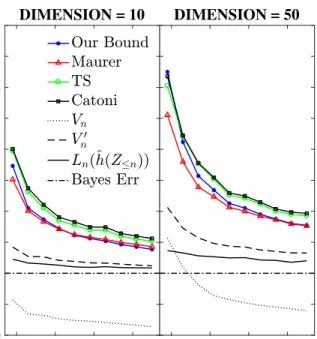
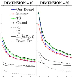
In this section, we experimentally compare our bound in Theorem3to that of TS [38], Catoni [8, Theorem 1.2.8] (withα=2), and Maurer in (2). For the latter, givenLn(Pn)∈[0,1[and the RHS of (2), we solve for an upper bound ofL(Pn)by “inverting” thekl. We note that TS [38] do not claim that their bound is better than Maurer’s in classification (in fact, they do better in other settings).

1000 3000 5000 7000 SAMPLE SIZE 0 0.1 0.2 0.3 0.4 0.5 0.6 BOUND DIMENSION = 10 1000 3000 5000 7000 SAMPLE SIZE DIMENSION = 50

Figure 1: Results for the synthetic data.

UCI d Test

err. Our Maurer Dataset ofˆ_{h bound bound} Haberman 3 0.272 0.521 0.411 (n=244) Breast-C. 9 0.068 0.185 0.159 (n=560) TicTacToe 27 0.046 0.191 0.216 (n=766) Banknote 4 0.058 0.125 0.136 (n=1098) kr-vs-kp 73 0.044 0.108 0.165 (n=2556) Spambase 57 0.173 0.293 0.312 (n=3680) Mushroom 116 0.002 0.018 0.055 (n=6500) Adult 108 0.168 0.195 0.234 (n=24130)

Table 1: Results for the UCI datasets. Setting.We consider both synthetic and real-world datasets for binary classification, and we evalu-ate bounds using the 0-1 loss. In particular, the data space_Zis_X×Y ∶=Rd_×{0,1}, whered∈N is the dimension of the feature space. In this case, the hypothesis setHis alsoRd_{, and the error} associated withh∈ Hon a sampleZ=(X, Y)∈ X_×Yis given byℓh(Z)=∣Y−1{φ(h

⊺

X)>1/2}∣, whereφ(w)∶=1/(1₊e−w_{), w∈R. We learn our hypotheses usingregularized logistic regression;} given a sampleS = (Zp, . . . , Zq), with (p, q) ∈ {(1, m),(m+1, n),(1, n)} andm = n/2, we compute ˆ h(S)∶=arg min h∈H λ∥h∥2 2 + 1 q₋p₊1 q ∑ i=p Yi⋅lnφ(h ⊺ Xi)+(1−Yi)⋅ln(1−φ(h ⊺ Xi)). (11)

ForZ_≤n∈ Zn_{, and1≤i≤m<j≤n, we choose algorithmQin Theorem3such that}

Q(Z_>i)≡δ(ˆh(Z>m)) and Q(Z<j)≡δ(ˆh(Z≤m)).

Given a sampleS≠∅, we set the “posterior”P(S)to be a Gaussian centered athˆ(S)with variance σ2

>0; that is,P(S)≡ N(ˆh(S), σ2

Id). The prior distribution is set toP0≡ N(0, σ 2

0Id), forσ0>0.

Parameters. We setδ =0.05. For all datasets, we useλ =0.01, and (approximately) solve (11)

using the BFGS algorithm. For each bound, we pick the σ2

∈ {1/2, . . . ,1/2J _{∶ J ∶=} ⌈_log

2n⌉}

which minimizes it on the given data (withninstances). In order for the bounds to still hold with probability at least1₋δ, we replaceδon the RHS of each bound byδ/⌈log2n⌉(this follows from

the application of a union bound). We choose the prior variance such thatσ2

0 = 1/2(this was the

best value on average for the bounds we compare against). We choose the gridGin Theorem3as in (9). Finally, we approximate Gaussian expectations using Monte Carlo sampling.

Synthetic data.We generate synthetic data ford={10,50}and sample sizes between 800 and 8000. For a given sample sizen, we 1) drawX1, . . . , Xn[resp.ǫ1, . . . , ǫn] identically and independently

from the multivariate-Gaussian distributionN(0, Id)[resp. the Bernoulli distributionB(0.9)]; and 2) we setYi=1{φ(h

⊺

∗Xi)>1/2}⋅ǫi, fori∈[n], whereh∗∈Rdis the vector constructed from the firstddigits ofπ. For example, ifd=10, thenh∗=(3,1,4,1,5,9,2,6,5,3)

⊺_{. Figure1shows the} results averaged over 10 independent runs for each sample size.

UCI datasets.For the second experiment, we use several UCI datasets. These are listed in Table1 (where Breast-C. stands for Breast Cancer). We encode categorical variables in appropriate 0-1 vectors. This effectively increases the dimension of the input space (this is reported asdin Table1). After removing any rows (i.e. instances) containing missing features and performing the encoding,

the input data is scaled such that every column has values between -1 and 1. We used a 5-fold train-test split (nin Table1is the training set size), and the results in Table1are averages over 5 runs. We only compare with Maurer’s bound since other bounds were worse than Maurer’s and ours on all datasets.

Discussion. As the dimensiondof the input space increases, the complexity KL(Pn∥P0)—and

thus, all the PAC-Bayes bounds discussed in this paper—get larger. Our bound suffers less from this increase ind, since for a large enough sample sizen, the termVnis small enough (see Figure1) to absorb any increase in the complexity. In fact, for large enoughn, the irreducible (complexity-free)

term involvingV′

nin our bound becomes the dominant one. This, combined with the fact that for the 0-1 loss,V′

n≈Ln(Pn)for large enoughn(see Figure1), makes our bound tighter than others. Adding a regularization term in the objective (11) is important as it stabilizesˆ_h(Z

<m)andˆh(Z≥m); a similar effect is achieved with methods like gradient descent as they essentially have a “built-in” regularization. For very small sample sizes, the regularization in (11) may not be enough to ensure thatˆ_h(Z

<m)andˆh(Z≥m)are close toˆh(Z≤n), in which caseVnneed not be necessarily small. In particular, this is the case for the Haberman and the breast cancer datasets where the advantage of our bound is not fully leveraged, and Maurer’s bound is smaller.

5

Theoretical Motivation of the Bound

In this section, we study the behavior of our bound (7) under a Bernstein condition:

Definition 6. [Bernstein Condition (BC)]The learning problem(D, ℓ,H) satisfies the (β, B) -Bernstein condition, forβ∈[0,1]andB>0, if for allh∈H,

E_Z∼D[(_ℓh(_Z)_−ℓh∗(_Z))2]≤_B⋅E_Z∼D[_ℓh(_Z)_−ℓh∗(_Z)]β_,

whereh∗∈arg inf_h∈HE_Z∼D[ℓ_h(Z)]is a risk minimizer within the closer ofH.

The Bernstein condition [2,4,5,14,21] essentially characterizes the “easiness” of the learning problem; it implies that the variance in the excess loss random variableℓh(Z)−ℓh∗(Z)gets smaller

the closer the risk of hypothesish ∈ Hgets to that of the risk minimizerh∗. For bounded loss functions, the BC withβ=0always holds. The BC withβ=1(the “easiest” learning setting) is also known as theMassart noise condition[24]; it holds in our experiment with synthetic data in Section 4, and also,e.g., wheneverHis convex andh↦ℓh(z)is exp-concave, for allz∈Z [14,30]. For more examples of learning settings where a BC holds see [21, Section 3].

Our aim in this section is to give an upper-bound on the infimum term involvingVnin (7), under a BC, in terms of the complexityCOMPnand the excess risksL¯(Pn),L¯(Q(Z>m)), andL¯(Q(Z≤m)), where for a distributionP∈P(H), the excess risk is defined by

¯

L(P)∶=E_h∼P[E_Z∼D[ℓh(Z)]]−EZ∼D[ℓh∗(Z)].

In the next theorem, we denoteQ_≤m∶=Q(Z≤m)andQ>m∶=Q(Z>m), form∈[n]. To simplify the presentation further (and for consistency with Section4), we assume thatQis chosen such that

Q(Z_>i)=Q_>m, for1≤i≤m, and Q(Z_<j)=Q_≤m, form<j≤n. (12) Theorem 7. Let G andπbe as in(9), δ ∈]0,1[, andεδ,n = 2 ln

1

δ⋅π(η) = 2 ln ∣G∣

δ , η ∈ G. If the

(β, B)-Bernstein condition holds withβ∈[0,1]andB>0, then for any learning algorithmsPand Q(withQsatisfying(12)), there exists aC>0, such that_∀n≥1andm=n/2, with probability at least1₋δ, 1 C⋅ηinf∈G{cη⋅Vn+ COMPn+εδ,n η⋅n }≤ ¯ L(Pn)+L¯(Q≤m)+L¯(Q>m) +(COMPn+εδ,n n ) 1 2−β +COMPn+εδ,n n . (13)

In addition to the “ESI” tools provided in Section6and Lemma13, the proof of Theorem7, pre-sented in AppendixE, also uses an “ESI version” of the Bernstein condition due to [21].

First note that the only terms in our main bound (7), other than the infimum on the LHS of (13), are the empirical errorLn(Pn)and aO˜(1/√n)-complexity-free term which is typically smaller than

√

KL₍Pn∥P0)/n(e.g. when the dimension ofHis large enough). The term

√

KL₍Pn∥P0)/nis

often the dominating one in other PAC-Bayesian bounds whenlim infn→∞Ln(Pn)>0.

Now consider the remaining term in our main bound, which matches the infimum term on the LHS of (13), and let us choose algorithmP as per Remark5, so thatCOMPn =2KL(Pn∥P0). Suppose

that, with high probability (w.h.p.), KL(Pn∥P0)/nconverges to 0 forn_→ ∞(otherwise no

PAC-Bayesian bound would converge to 0), then₍COMPn/n)1/(2−β)+COMPn/n—essentially the sum of the last two terms on the RHS of (13)—converges to 0 at a faster rate than√KL₍Pn∥P0)/nw.h.p.

forβ>0, and at equal rate forβ=0. Thus, in light of Theorem7, to argue that our bound can be better than others (still whenlim infn→∞Ln(Pn)>0), it remains to show that there exist algorithms

PandQfor which the sum of the excess risks on the RHS of (13) is smaller than√KL(Pn∥P0)/n.

One choice of estimator with small excess risk is the Empirical Risk Minimizer (ERM). When m= n/2, if one choosesQsuch that it outputs a Dirac around the ERM on a given sample, then under a BC with exponentβ and for “parametric”H(such as thed-dimensional linear classifiers

in Sec. 4), _L¯_(Q

≤m)andL¯(Q>m)are of order O˜(n−1/(2−β))w.h.p. [2,18]. However, setting

Pn≡δ(ERM(Z≤n))is not allowed, since otherwise KL(Pn∥P0)=∞. Instead one can chooseP_n

to be the generalized-Bayes/Gibbs posterior. In this case too, under a BC with exponentβ and for

parametricH, the excess risk is of order_O˜_(n−1_/(2−β))_{w.h.p. for clever choices of prior}

P0[2,18].

6

Detailed Analysis

We start this section by presenting the convenient ESI notation and use it to present our main tech-nical Lemma13(proofs of the ESI results are in AppendixD). We then continue with a proof of Theorem3.

Definition 8. [ESI (Exponential Stochastic Inequality, pronounce as:easy)18,21]Letη>0, and X,Y be any two random variables with joint distributionD. We define

X⊴D_η Y ⇐⇒ X−Y ⊴ηD 0 ⇐⇒ E(X,Y)∼D[eη(X

−Y)_{]≤1. (14)} Definition8can be extended to the case whereη =ηˆis also a random variable, in which case the expectation in (14) needs to be replaced by the expectation over the joint distribution of (X,Y,ηˆ). When no ambiguity can arise, we omitDfrom the ESI notation. Besides simplifying notation, ESIs

Proposition 9. [ESI Implications]For fixedη>0, ifX ⊴η Y thenE[X]≤E[Y]. For both fixed

and randomη, ifˆ X⊴_ηˆY, then∀δ∈]0,1[,X ≤Y + ln1

δ

ˆ

η , with probability at least1−δ.

In the next proposition, we present two results concerning transitivity and additive properties of ESI: Proposition 10. [ESI Transitivity and Chain Rule](a) LetZ1, . . . , Zn be any random variables

onZ(not necessarily independent). If for some(γi)i∈[n]∈]0,+∞[n,Zi⊴γi0, for alli∈[n], then n ∑ i=1 Zi⊴νn0, whereνn∶=( n ∑ i=1 1 γi) −1 (so if_∀i∈[n], γi=γ>0thenνn=γ/n). (15)

(b) Suppose now thatZ1, . . . , Znare i.i.d. and letX∶Z×⋃n_i=1Zi→Rbe any real-valued function.

If for someη>0,X(Zi;z<i)⊴η0, for alli∈[n]and allz<i∈Zi−1, then∑ni=1X(Zi;Z<i)⊴η0. We now give a basic PAC-Bayesian result for the ESI context:

Proposition 11. [ESI PAC-Bayes]Fixη>0and let{Yh∶h∈H}be any family of random variables

such that for allh∈H,Yh⊴η0. LetP0be any distribution onHand letP∶⋃n_i=1Zi→P(H)be a

learning algorithm. We have:

E_h∼Pn[Yh]⊴η

KL₍Pn∥P0)

η , wherePn∶=P(Z≤n).

In many applications (especially for our main result) it is desirable to work with a random (i.e.

data-dependent)ηin the ESI inequalities; one can tuneηafter seeing the data.

Proposition 12. [ESI from fixed to randomη] LetGbe a countable subset of]0,_+∞[and let πbe a prior distribution overG. Given a countable collection{Yη ∶ η ∈ G}of random variables

satisfyingYη⊴η0, for all fixedη∈G, we have, for arbitrary estimatorηˆwith support onG,

Y_ηˆ⊴_ηˆ −

lnπ(ηˆ) ˆ

η . (16)

The following key lemma, which is of independent interest, is central to our main result.

Lemma 13. [Key result:un-expected Bernstein]LetX∼Dbe a random variable bounded from

abovebyb>0almost surely, and letϑ(u)∶=(−ln(1₋u)−u)/u2

. For all0<η<1/b, we have(a):

E[X]₋X ⊴D_η c_⋅X2, for allc≥η_⋅ϑ(ηb). (17)

(b): The result is tight; for everyc<η⋅ϑ(ηb), there exists a distributionDso that (17) does not hold.

Lemma13is reminiscent of the following slight variation of Bernstein’s inequality [11]; letX be

any random variable bounded frombelowby₋b, and letκ(x)∶=(ex_−x−1)/_x2

. For allη>0, we have

E[_X]_−X⊴_{η s⋅}E[_X2]_, for all_s≥_η⋅κ(_ηb). (18) Note that the un-expected Bernstein Lemma13has theX2

lifted out of the expectation. In Appendix

G, we prove (18) and compare it to standard versions of Bernstein. We also compare (17) to the related but distinct empirical Bernstein inequality due to [26, Theorem 4]. We now prove part (a) of Lemma13, which follows easily from the proof of an existing result [15,20]. Part (b) is novel; its proof is postponed to AppendixF.

Proof of Lemma13-Part (a). [15] (see also [20]) showed in the proof of their lemma 4.1 that exp(λξ−λ2ϑ(λ)ξ2)≤1₊λξ, for allλ∈[0,1[ and ξ≥−1. (19)

Lettingη=λ/bandξ=₋X/b, (19) becomes,

exp(₋ηX₋η2ϑ(ηb)X2)≤1₋ηX, for allη∈]0,1/b[. (20) Taking expectation on both sides of (20) and using the fact that1₋ηE[_X]≤exp(₋ηE[_X])on the RHS of the resulting inequality, leads to (17).

Proof of Theorem3. Letη∈]0,1/b[andcη∶=η⋅ϑ(ηb). For1≤i≤m<j≤n, define Xh(Zi;z>i)∶=ℓh(Zi)−Eh′_∼Q(z >i)[ℓh′(Zi)], forz>i∈Z n−i_, ˜ Xh(Zj;z<j)∶=ℓh(Zj)−Eh′_∼Q(z <j)[ℓh′(Zj)], forz<j∈Z j−1 .

Sinceℓis bounded from above byb, Lemma13implies that for allh∈Hand1≤i≤m<j≤n,

∀z_>i∈Zn−i_{, Y}η

h(Zi;z>i)∶=EZ′

i∼D[Xh(Z ′

i;z>i)]−Xh(Zi;z>i)−cη⋅Xh(Zi;z>i)

2 ⊴η0, ∀z_<j∈Zj−1 , Y˜_hη(Zj;z<j)∶=FZ′ j∼D[ ˜ Xh(Z ′ j;z<j)]−X˜h(Zj;z<j)−cη⋅X˜h(Zj;z<j) 2 ⊴η0, SinceZ1, . . . , Z_nare i.i.d. we can chain the ESIs above using Proposition10-(b) to get:

S∶=∑m i=1 Y_hη(Zi;Z>i)⊴η0, S˜∶= n ∑ j=m+1 ˜ Y_hη(Zj;Z<j)⊴η0. (21) Applying PAC-Bayes (Proposition11) toSand_S˜_{in (21) with priorsP(Z}

>m)andP(Z≤m), respec-tively, and common posteriorPn = P(Z≤n)onH, we get, with KL>m ∶= KL(Pn∥P(Z>m))and KL≤m∶=KL(Pn∥P(Z≤m)): E_h∼Pn[ m ∑ i=1 Y_hη(Zi;Z>i)]− KL_>m η ⊴η0, Eh∼Pn ⎡⎢ ⎢⎢ ⎣ n ∑ j=m+1 ˜ Y_hη(Zj;Z<j)⎤⎥⎥⎥ ⎦− KL_≤m η ⊴η0.

We now apply Proposition10-(a) to chain these two ESIs, which yields E_h∼Pn⎡⎢⎢⎢ ⎣ m ∑ i=1 Y_hη(Zi;Z>i)+ n ∑ j=m+1 ˜ Y_hη(Zj;Z<j)⎤⎥⎥⎥ ⎦⊴η2 KL₍Pn∥P(Z>m))+KL(Pn∥P(Z≤m)) η .

With the priorπonG, we have for anyηˆ=ηˆ(Z_≤n)∈G⊂[1/

√ nb2 ,1/b[(see Proposition12), E_h∼Pn⎡⎢⎢⎢ ⎣ m ∑ i=1 Y_hηˆ(Zi;Z>i)+ n ∑ j=m+1 ˜ Y_hηˆ(Zj;Z<j)⎤⎥⎥⎥ ⎦⊴η2ˆ COMP_n ˆ η − 2 lnπ(ηˆ) ˆ η , i.e., n_⋅(L(Pn)−Ln(Pn)) ⊴ηˆ 2 n_⋅c_ηˆ⋅V_n+ COMP_n+2 ln 1 π(_ηˆ₎ ˆ η + ⎡⎢ ⎢⎢ ⎣ m ∑ i=1 (E_Z′ i∼D[ℓ¯Q>i(Z ′ i)]−ℓ¯Q>i(Zi))+ n ∑ j=m+1 (E_Z′ j∼D[ℓ¯Q<j(Z ′ j)]−ℓ¯Q<j(Zj))⎤⎥⎥⎥ ⎦,(22) where_ℓ¯

Q>i(Zi) ∶= Eh∼Q(Z>i)[ℓh(Zi)] andℓ¯Q<j(Zj) ∶= Eh∼Q(Z<j)[ℓh(Zj)]. LetUn denote the quantity between the square brackets in (22). Using the un-expected Bernstein Lemma13, together with Proposition16, we get for any estimatorνˆonG:

Un⊴ˆ_ν c_νˆ⋅⎛ ⎝ m ∑ i=1 E_h′_∼Q(Z >i)[ℓh′(Zi) 2 ]+ n ∑ j=m+1 E_h′_∼Q(Z <j)[ℓh′(Zj) 2 ]⎞_⎠+ln 1 π(_νˆ₎ ˆ ν . (23)

By chaining (23) and (22) using Proposition10-(a) and dividing byn, we get: L(Pn)⊴nηˆνˆ ˆ η+2 ˆν Ln(Pn)+c ˆ η⋅Vn+ COMPn+2 ln 1 π(ηˆ) ˆ η_⋅n +cνˆ⋅V ′ n+ ln 1 π(νˆ) ˆ ν_⋅n . (24)

We now apply Proposition9to (24) to obtain the following inequality with probability at least1₋δ:

L(Pn)≤Ln(Pn)+ ⎡⎢ ⎢⎢ ⎢⎣c_ηˆ⋅V_n+ COMP_n+2 ln 1 π(_ηˆ₎⋅δ ˆ η_⋅n ⎤⎥ ⎥⎥ ⎥⎦+⎧⎪⎪⎨⎪⎪⎩c ˆ ν⋅V ′ n+ ln 1 π(_νˆ₎⋅δ ˆ ν_⋅n ⎫⎪⎪ ⎬⎪⎪ ⎭. (25)

Inequality (7) follows after pickingνˆandηˆto be, respectively, estimators which achieve the infimum over the closer of_Gof the quantities between braces and square brackets in (25).

7

Conclusion and Future Work

The main goal of this paper was to introduce a new PAC-Bayesian bound based on a new proof technique; we also theoretically motivated the bound in terms of a Bernstein condition. The simple experiments we provided are to be considered as a basic sanity check—in future work, we plan to put the bound to real practical use by applying it to deep nets in the style of,e.g., [41].

Acknowledgments

An anonymous referee made some highly informed remarks on our paper, which led us to substan-tially rewrite the paper and made us understand our own work much better. Part of this work was performed while Zakaria Mhammedi was interning at the Centrum Wiskunde & Informatica (CWI). This work was also supported by the Australian Research Council and Data61.

References

[1] Pierre Alquier and Benjamin Guedj. Simpler PAC-Bayesian bounds for hostile data.Machine Learning, 107(5):887–902, 2018.

[2] Jean-Yves Audibert. PAC-Bayesian statistical learning theory. These de doctorat de l’Université Paris, 6:29, 2004.

[3] Jean-Yves Audibert, Rémi Munos, and Csaba Szepesvári. Tuning bandit algorithms in stochas-tic environments. InInternational conference on algorithmic learning theory, pages 150–165.

Springer, 2007.

[4] Peter L. Bartlett, Michael I. Jordan, and Jon D. McAuliffe. Convexity, classification, and risk bounds. Journal of the American Statistical Association, 101(473):138–156, 2006.

[5] Peter L. Bartlett and Shahar Mendelson. Empirical minimization. Probability Theory and Related Fields, 135(3):311–334, 2006.

[6] Olivier Bousquet and André Elisseeff. Stability and generalization.Journal of machine learn-ing research, 2(Mar):499–526, 2002.

[7] Olivier Catoni. A PAC-Bayesian approach to adaptive classification.preprint, 2003.

[8] Olivier Catoni. PAC-Bayesian Supervised Classification. Lecture Notes-Monograph Series.

IMS, 2007.

[9] Olivier Catoni. PAC-Bayesian supervised classification: the thermodynamics of statistical learning. Lecture Notes-Monograph Series. IMS, 2007.

[10] Nicolo Cesa-Bianchi, Yishay Mansour, and Gilles Stoltz. Improved second-order bounds for prediction with expert advice.Machine Learning, 66(2-3):321–352, 2007.

[11] Nicolò Cesa-Bianchi and Gàbor Lugosi.Prediction, Learning and Games. Cambridge

Univer-sity Press, Cambridge, UK, 2006.

[12] Dheeru Dua and Casey Graff. UCI machine learning repository, 2017.

[13] Gintare K. Dziugaite and Daniel M. Roy. Computing nonvacuous generalization bounds for deep (stochastic) neural networks with many more parameters than training data. InUAI, 2017.

[14] Tim Van Erven, Nishant A. Mehta, Mark D. Reid, and Robert C. Williamson. Fast rates in statistical and online learning.Journal of Machine Learning Research, 16:1793–1861, 2015.

[15] Xiequan Fan, Ion Grama, Quansheng Liu, et al. Exponential inequalities for martingales with applications. Electronic Journal of Probability, 20, 2015.

[16] Pascal Germain, Alexandre Lacasse, François Laviolette, and Mario Marchand. PAC-Bayesian learning of linear classifiers. InProceedings of the 26th Annual International Conference on Machine Learning, pages 353–360. ACM, 2009.

[17] Pascal Germain, Alexandre Lacasse, Francois Laviolette, Mario Marchand, and Jean-Francis Roy. Risk bounds for the majority vote: From a pac-bayesian analysis to a learning algorithm.

The Journal of Machine Learning Research, 16(1):787–860, 2015.

[18] Peter D. Grünwald and Nishant A. Mehta. Fast rates for general unbounded loss functions: from ERM to generalized Bayes. Journal of Machine Learning Research, 2019.

[19] Benjamin Guedj. A primer on PAC-Bayesian learning. arXiv preprint arXiv:1901.05353,

2019.

[20] Steven R Howard, Aaditya Ramdas, Jon McAuliffe, and Jasjeet Sekhon. Uniform, nonpara-metric, non-asymptotic confidence sequences. arXiv preprint arXiv:1810.08240, 2018.

[21] Wouter M. Koolen, Peter D. Grünwald, and Tim van Erven. Combining adversarial guarantees and stochastic fast rates in online learning. In Advances in Neural Information Processing Systems, pages 4457–4465, 2016.

[22] John Langford and Rich Caruana. (Not) bounding the true error. In T. G. Dietterich, S. Becker, and Z. Ghahramani, editors, Advances in Neural Information Processing Systems 14, pages

809–816. MIT Press, 2002.

[23] John Langford and John Shawe-Taylor. PAC-Bayes & margins. InAdvances in Neural Infor-mation Processing Systems, pages 439–446, 2003.

[24] Pascal Massart and Élodie Nédélec. Risk bounds for statistical learning. The Annals of Statis-tics, 34(5):2326–2366, 2006.

[25] Andreas Maurer. A note on the PAC-Bayesian theorem. arXiv preprint cs/0411099, 2004.

[26] Andreas Maurer and Massimiliano Pontil. Empirical Bernstein bounds and sample variance penalization. InProceedings COLT 2009, 2009.

[27] David A. McAllester. Some PAC-Bayesian theorems. InProceedings of the Eleventh ACM Conference on Computational Learning Theory (COLT’ 98), pages 230–234. ACM Press,

1998.

[28] David A. McAllester. PAC-Bayesian model averaging. InProceedings of the Twelfth ACM Con-ference on Computational Learning Theory (COLT’ 99), pages 164–171. ACM Press, 1999.

[29] David A. McAllester. PAC-Bayesian stochastic model selection. Machine Learning, 51(1):5–

21, 2003.

[30] Nishant A. Mehta. Fast rates with high probability in exp-concave statistical learning. In

Artificial Intelligence and Statistics, pages 1085–1093, 2017.

[31] Volodymyr Mnih, Csaba Szepesvári, and Jean-Yves Audibert. Empirical bernstein stopping. In

Proceedings of the 25th international conference on Machine learning, pages 672–679. ACM,

2008.

[32] Sayan Mukherjee, Partha Niyogi, Tomaso Poggio, and Ryan Rifkin. Learning theory: stability is sufficient for generalization and necessary and sufficient for consistency of empirical risk minimization.Advances in Computational Mathematics, 25(1-3):161–193, 2006.

[33] Behnam Neyshabur, Srinadh Bhojanapalli, David A. McAllester, and Nathan Srebro. A PAC-Bayesian approach to spectrally-normalized margin bounds for neural networks. In ICLR,

2018.

[34] Omar Rivasplata, Csaba Szepesvári, John S Shawe-Taylor, Emilio Parrado-Hernandez, and Shiliang Sun. Pac-bayes bounds for stable algorithms with instance-dependent priors. In

Advances in Neural Information Processing Systems, pages 9214–9224, 2018.

[35] Matthias Seeger. PAC-Bayesian generalisation error bounds for Gaussian process classification.

Journal of machine learning research, 3(Oct):233–269, 2002.

[36] Matthias Seeger. PAC-Bayesian generalization error bounds for Gaussian process classifica-tion. Journal of Machine Learning Research, 3:233–269, 2002.

[37] Shai Shalev-Shwartz, Ohad Shamir, Nathan Srebro, and Karthik Sridharan. Learnability, sta-bility and uniform convergence. Journal of Machine Learning Research, 11(Oct):2635–2670,

2010.

[38] Ilya O. Tolstikhin and Yevgeny Seldin. PAC-Bayes-empirical-Bernstein inequality. In Ad-vances in Neural Information Processing Systems, pages 109–117, 2013.

[39] Alexandre B. Tsybakov. Optimal aggregation of classifiers in statistical learning. The Annals of Statistics, 32(1):135–166, 2004.

[40] Olivier Wintenberger. Optimal learning with bernstein online aggregation.Machine Learning,

106(1):119–141, 2017.

[41] Wenda Zhou, Victor Veitch, Morgane Austern, Ryan P. Adams, and Peter Orbanz. Non-vacuous generalization bounds at the ImageNet scale: a PAC-Bayesian compression approach. InICLR, 2019.

A

Informed Priors

Any bound of the form of (1) with COMP_n = KL(Pn∥P0)can be applied in a way as to replace

this KL term by KL₍Pn∥P(Z>m))+KL(Pn∥P(Z≤m)), and thus making use of “informed priors”. For this, it suffices to apply the bound on each part of the sample, i.e. Z_>mandZ≤m, and then combine the resulting bounds with a union bound. In fact, suppose that (1) holds withRn=Ln(Pn) andC=0, and let_δ∈]0,1[. Applying the bound on the second part of the sampleZ>mwith prior

P(Z_≤m)and posteriorPn, we get, with probability at least1−δ,

L(Pn)−L>m(Pn)≤P⋅ √ L_>m(Pn)⋅(KL(Pn∥P(Z≤m))+εδ,n−m) n−m +A_⋅KL(Pn∥P(Z≤m))+εδ,n−m n₋m , (26) whereL_>m(Pn)∶= 1 n−m∑ n

j=m+1Eh∼Pn[ℓh(Zj)]. Similarly, applying the bound on the first half of the sampleZ_≤mwith priorP(Z>m)and posteriorPn, we get, with probability at least1−δ,

L(Pn)−L≤m(Pn)≤P⋅ √ L_≤m(Pn)⋅(KL(Pn∥P(Z>m))+εδ,m) m +A_⋅ KL(Pn∥P(Z>m))+εδ,m m , (27) whereL_≤m(Pn)∶= 1 m∑ m

i=1Eh∼Pn[ℓh(Zi)]. Letp∶=m/nandq∶=(n−m)/n(note thatp+q=1). Applying a union bound and addingq×(26) withp×(27), yields the bound

L(Pn)−Ln(Pn)≤P⋅ √ 2Ln(Pn)⋅(KL(Pn∥P(Z>m))+KL(Pn∥P(Z≤m))+ε¯δ,n) n +A_⋅KL(Pn∥P(Z>m))+KL(Pn∥P(Z≤m))+ε¯δ,n n , (28)

with probability at least1₋δ, whereε¯δ,n∶=εδ/2_,m+ε_δ/2_,n−m. To get to (28), we also used the fact that√x₊√y≤√2(x₊y), for allx, y∈R_≥0.

The above trick does not directly apply to Maurer’s bound in (2) (since the dependence onL(Pn)is not linear). Instead, one can use the joint convexity of the binary Kullback-Leibler divergenceklin its two arguments as in the following proof of Lemma4:

Proof of Lemma4. Letδ∈]0,1[. We can writeLn(Pn)as

Ln(Pn)= p m m ∑ i=1 E_h∼Pn[ℓh(Zi)]+ q n−m n ∑ j=m+1 E_h∼Pn[ℓh(Zj)],

wherep∶=m/nandq∶=(n−m)/n(note thatp+q=1). Let us denote L_≤m(Pn)∶= 1 m m ∑ i=1 E_h∼Pn[ℓh(Zi)] and L>m(Pn)∶= 1 n−m n ∑ j=m+1 E_h∼Pn[ℓh(Zj)].

By the joint convexity of the binary Kullback-Leibler divergenceklin its two arguments, we have kl(L(Pn)∥Ln(Pn))=kl(pL(Pn)+qL(Pn)∥pL≤m(Pn)+qL>m(Pn)), ≤p⋅kl(L(Pn)∥L≤m(Pn))+q⋅kl(L(Pn)∥L>m(Pn)), ≤p_⋅ KL(Pn∥P(Z>m))+ln 4√_m δ m , +q⋅ KL(Pn∥P(Z≤m))+ln 4√_n−m δ n₋m , (29)

with probability at least1₋δ, where the last inequality follows by Maurer’s bound (2) and the union

B

Biasing

A PAC-Bayes bound similar to the one in our Corollary1can be obtained from the TS bound. For this, the TS bound must be applied twice, once on each part of the sample (i.e. Z_≤mandZ>m) to

biasedlosses. We demonstrate this in what follows.

Letˆ_{h∶ ⋃}n

i=1Zi → Hbe any estimator. The TS bound can be expressed in the form of (1) with

COMPn = KL(Pn∥P0),C= 0, andR_n =E_h∼Pn[Var_n[ℓ_h(Z)]], whereVar_n[X]denotes the

em-pirical variance. Applying the TS bound on the second part of the sampleZ_>mwith priorP0and

posteriorPn, and with the biased lossℓ˜h(Z)=ℓh(Z)−ℓˆ

h(Z≤m)(Z), gives ˜ L(Pn)−L˜>m(Pn)≤P⋅ √ E_h∼Pn[Var_>m[ℓ˜h(Z)]]⋅(KL(Pn∥P0)+εδ,n−m) n−m +A_⋅ KL(Pn∥P0)+εδ,n−m n₋m , (30)

with probability at least1₋δ, whereVar_>m[X]∶= 1

n−m∑ n i=m+1(Xi− 1 n−m∑ n j=m+1Xj) 2 ,_L˜_(P n)∶= E_h∼Pn[E_Z∼D[_ℓ˜_h(_Z)]], and_L˜_>m(_Pn)_∶= 1 n−m∑ n j=m+1Eh∼Pn[ℓ˜h(Zj)].

Doing the same on the first part of the sampleZ≤m, but now with the loss _ℓˇ

h(Z) ∶= ℓh(Z)− ℓˆ h(Z>m)(Z), yields ˇ L(Pn)−Lˇ≤m(Pn)≤P⋅ √ E_h∼Pn[Var_≤m[ℓˇh(Z)]]⋅(KL(Pn∥P0)+ε_δ,m) m +A_⋅KL(Pn∥P0)+εδ,m m , (31)

with probability at least 1 ₋ δ, where Var_≤m[X] ∶=

1 m∑ m i=1(Xi− 1 m∑ m j=1Xj) 2 , _Lˇ_{(Pn) ∶=} E_h∼Pn[E_Z∼D[_ℓˇ_h(_Z)]], and_Lˇ_≤m(_Pn)_∶= 1 m∑ m i=1Eh∼Pn[ℓˇh(Zi)].

Two more applications of the TS bound with prior and posterior equal toP0, yields,

L(ˆh(Z_≤m))₋L_>m(ˆh(Z_≤m))≤P_⋅ ¿ Á Á ÀVar_>m[ℓˆ h(Z≤m)(Z)]⋅εδ/2,n−m n−m + A_⋅εδ/2_,n−m n−m , and (32) L(ˆh(Z>m))−L≤m(ˆh(Z>m))≤P⋅ ¿ Á Á ÀVar_≤m[ℓˆ_h(Z >m)(Z)]⋅εδ/2,m m + A_⋅εδ/2_,m m , (33)

with probability at least1₋δ, where L_≤m(ˆh(Z_>m))∶= 1 m m ∑ i=1 ℓˆ_h(Z >m)(Zi) and L>m( ˆ h(Z_≤m))∶= 1 n−m n ∑ j=m+1 ℓ_hˆ_(Z ≤m)(Zj). Letp=m/nandq=(n−m)/n. Applying a union bound and combining (30)-(33), as

q×((30)+(32)₎+p×((31)+(33)₎,

yields a bound of the form (1) with

R′ n=p⋅Var≤m[ℓˆ h(Z>m)(Z)]+q⋅Var<m[ℓˆh(Z≤m)(Z)]≤V ′ n, Rn=p⋅Eh∼Pn[Var≤m[ℓˇh(Z)]]+q⋅Eh∼Pn[Var>m[ℓ˜h(Z)]]≤Vn, whereV′

nandVnare as in Corollary1.

A Direct Approach. Though the steps above lead to a bound similar to ours in Corollary1, the constants involved may not be optimal. We now re-derive a modification of the TS bound with aVn term like in Corollary1, and with tighter constants. The proof techniques used here are the same as those used in the proof of Theorem3. Forη∈]0,1/b[(whereb>0is an upper-bound on the lossℓ)

andm∈[2..n], define sη∶=η⋅κ(ηb), where κ(η)∶=(eη−η−1)/η 2 , and c˜η∶= sηm 2m−2(1+ ηm 2m−2) −1 , λ(η)∶= ηβ(η) η+β(η), whereβ(η)∶=η+ η2 m2 2m−2.

We assume thatn>2is even in the next theorem. We remind the reader of the definitions Var_≤m[X]∶= 1 m m ∑ i=1 ⎛ ⎝Xi− 1 m m ∑ j=1 Xj⎞ ⎠ 2 andVar_>m[X]∶= 1 n−m n ∑ i=m+1 ⎛ ⎝Xi− 1 n−m n ∑ j=m+1 Xj⎞ ⎠ 2 .

Theorem 14. [New PAC-Bayes Empirical Bernstein Bound]LetZ1, . . . , Znbe i.i.d. withZ1∼D.

Letm= n/2> 1andπbe any distribution with support on a finite or countable gridG ⊂]0,1/b[. For anyδ ∈]0,1[, learning algorithmP ∶ ⋃n

i=1Zi →P(H), and estimatorˆh∶ ⋃ni=1Zi → H, we have, L(Pn)≤Ln(Pn)+inf η∈G ⎧⎪⎪ ⎨⎪⎪ ⎩˜cη⋅Gn+ COMPn+2 ln 1 δ⋅π(η) λ(η)⋅n ⎫⎪⎪ ⎬⎪⎪ ⎭+ν∈Ginf ⎧⎪⎪ ⎨⎪⎪ ⎩c˜ν⋅G ′ n+ ln 1 δ⋅π(ν) λ(ν)⋅n ⎫⎪⎪ ⎬⎪⎪ ⎭, with probability at least1₋δ, whereCOMP_n,G′

n, andGnare the random variables defined by:

COMP_n∶=KL(Pn∥P(Z≤m))+KL(Pn∥P(Z>m)), G′ n∶=Var>m[ℓˆ_h(Z ≤m)(Z)]+Var≤m[ℓˆh(Z>m)(Z)], Gn∶=Eh∼Pn[Var>m[ℓh(Z)−ℓˆ h(Z≤m)(Z)]+Var≤m[ℓh(Z)−ℓˆh(Z>m)(Z)]]. Note that sinceVar_≤m(X)≤ ∑mi=1X

2 i/mandVar>m(X)≤ ∑ni=m+1X 2 i/m, we have Gn≤Vn and G′n≤V ′ n,

whereVn andVn′ are defined in (5) and (4), respectively. However, one cannot directly compare

Gnto theVndefined in Theorem3, since the latter uses “online” posteriors(Q(Z>i))andQ(Z<j) which get closer and closer to the posteriorQ(Z_≤n)based on the full sample.

To prove Theorem14, we need the following self-bounding property of the empirical variance [26]:

mVar[X]⊴η

m2

m−1Varm[X]−

ηm2

2m−2Var[X], (34) for any η > 0 and any bounded random variable X, where Varm[X] is either Var_>m[X] or Var_≤m[X](recall thatm = n/2). Re-arranging (34) and dividing by(1₊ηm/(2m₋2)), leads to mVar[X]⊴β(η) m 2 m₋1⋅(1+ ηm 2m₋2) −1 Varm[X], (35) where β(η)∶=η+ η 2 m 2m−2. Proof of Theorem14. Letη∈]0,1/b[andsη∶=η⋅κ(ηb). We define

Xh(Zi)∶=ℓh(Zi)−ℓˆ_h(Z

>m)(Zi), for 1≤i≤m, ˜

Xh(Zj)∶=ℓh(Zj)−ℓˆ_h(Z

≤m)(Zj), for m<j≤n.

Sinceℓis bounded from above byb, the Bernstein inequality (18) applied to the zero-mean random

variablesE_Z′

i∼D[Xh(Zi′)]−Xh(Zi), i∈[n],implies that for allh∈H,

Y_hη(Zi)∶=EZ_i∼′ _D[X_h(Z′

i)]−Xh(Zi)−sη⋅Var[Xh(Z)]⊴η0, for 1≤i≤m, ˜

Y_hη(Zj)∶=EZ_j∼′ _D[X˜_h(Z′

j)]−X˜h(Zj)−sη⋅Var[X˜h(Z)]⊴η0, for m<j≤n. SinceZ1, . . . , Z_nare i.i.d. we can chain the ESIs above using Proposition10-(b) to get:

S∶=∑m i=1 Y_hη(Zi)⊴η0, S˜∶= n ∑ j=m+1 ˜ Y_hη(Zj)⊴η0.

ChainingS ⊴η 0 [resp. S˜ ⊴η 0] and (35) with Varm ≡ Var≤m [resp. Varm ≡ Var>m] using Proposition10-(a), yields,

W_hη⊴ηβ(η) η+β(η) 0 and _W˜η h ⊴ηβ(η) η+β(η) 0, where (36) W_hη∶=∑m i=1 (E_Z′ i∼D[Xh(Z ′ i)]−Xh(Zi))− sηm2 m−1⋅(1+ ηm 2m−2) −1 Var_≤m[Xh(Z)], ˜ W_hη∶= ∑n j=m+1 (E_Z′ j∼D[Xh(Z ′ j)]−Xh(Zj))− sηm 2 m−1⋅(1+ ηm 2m−2) −1 Var_>m[Xh(Z)]. Letλ(η)∶=ηβ(η)/(β(η)+η). Applying PAC-Bayes (Proposition11) toW_hη⊴λ(η)0andW˜hη⊴λ(η) 0in (36), with priorsP(Z_>m)andP(Z≤m), respectively, and posteriorPn=P(Z≤n)onH, we get:

E_h∼Pn[W_hη]₋KL(Pn∥P(Z>m))

λ(η) ⊴λ(η)0, Eh∼Pn[

˜

W_hη]₋KL(Pn∥P(Z≤m))

λ(η) ⊴λ(η)0.

We now apply Proposition10-(a) to chain these two ESIs, which yields E_h∼Pn[_Wη h +W˜ η h]⊴λ(η) 2 KL₍Pn∥P(Z>m))+KL(Pn∥P(Z≤m)) λ(η) .

With the discrete priorπonG, we have for anyηˆ=ηˆ(Z_≤n)∈G⊂1/b_⋅[1/√n,1[(see Proposition

12), E_h∼Pn[W_hη₊W˜_hη]⊴λ(ηˆ) 2 COMPn λ(ηˆ) − 2 lnπ(ηˆ) λ(ηˆ) , i.e., n_⋅(L(Pn)−Ln(Pn)) ⊴λ(ˆη) 2 n_⋅˜c_ηˆ⋅G_n+ COMP_n+2 ln 1 π(_ηˆ₎ λ(ηˆ) + ⎡⎢ ⎢⎢ ⎣ m ∑ i=1 (E_Z′ i∼D[ℓˆh>m(Z ′ i)]−ℓˆ_h >m(Zi))+ n ∑ j=m+1 (E_Z′ j∼D[ℓhˆ≤m(Z ′ j)]−ℓˆ_h ≤m(Zj)) ⎤⎥ ⎥⎥ ⎦, (37) where_hˆ

>m∶=ˆh(Z>m)andˆh≤m∶=ˆh(Z≤m). LetUndenote the quantity between the square brackets in (37). Using the Bernstein inequality in (18) chained with (35), and Proposition16, we get for any estimatorνˆonG: Un⊴λ(ˆ_ν) n⋅˜cνˆ⋅(Var≤m[ℓˆ_h(Z >m)(Z)]+Var>m[ℓˆh(Z≤m)(Z)])+ ln 1 π(νˆ) λ(νˆ) . (38)

By chaining (37) and (38) using Proposition10-(a), dividing byn, we get: L(Pn)⊴nλ(ηˆ)λ(ˆν) λ(ηˆ)+2λ(ˆν) Ln(Pn)+c˜ηˆ⋅Gn+ COMPn+2 ln 1 π(_ηˆ₎ λ(ηˆ)⋅n +c˜ˆν⋅G ′ n+ ln 1 π(_νˆ₎ λ(νˆ)⋅n. (39)

We now apply Proposition9to (39) to obtain the following inequality with probability at least1₋δ:

L(Pn)≤Ln(Pn)+⎡⎢⎢⎢ ⎢⎣˜c_ηˆ⋅G_n+ COMPn+2 ln 1 π(_ηˆ₎⋅δ λ(ηˆ)_⋅n ⎤⎥ ⎥⎥ ⎥⎦+⎧⎪⎪⎨⎪⎪⎩˜c ˆ ν⋅G ′ n+ ln 1 π(_νˆ₎⋅δ λ(νˆ)_⋅n ⎫⎪⎪ ⎬⎪⎪ ⎭. (40)

Inequality (7) follows after pickingνˆandηˆto be, respectively, estimators which achieve the infimum over the closer of_Gof the quantities between braces and square brackets in (40).

C

Proof of Lemma

2

Proof. Throughout this proof, we denoteˆh_>m∶=ˆ_h(Z

>m)andˆh≤m∶=ˆh(Z≥m). Letδ∈]0,1[. Since the sampleZ_≤mis independent ofZ>m, we have

2 n m ∑ i=1 ℓˆ h>m(Zi) 2 =Var_≤m[ℓˆ h>m(Z)]+( 1 m m ∑ i=1 ℓˆ h>m(Zi)) 2 . (41)

On the other hand, from [26, Theorem 10], we have Var_≤m[ℓˆ_h >m(Z)]≤ 2(m−1) m Var[ℓˆh>m(Z)]+ 8 ln1 δ n , ∣ℓ∣≤1 ≤ 2(m−1) m L( ˆ h_>m)₊8 ln 1 δ n , (42)

with probability at least1₋δ. By Hoeffding’s inequality, we also have

(_m1 ∑m i=1 ℓˆ h>m(Zi)) 2 ≤2L(ˆh_>m) 2 +8 ln 1 δ n , ∣ℓ∣≤1 ≤ 2L(ˆh_>m)+ 8 ln1 δ n , (43)

with probability at least1−δ. Combining (41), (42), and (43) together using a union bound, yields

2 n m ∑ i=1 ℓˆ h>m(Zi) 2 ≤ 4(n−1) n L( ˆ h_>m)+ 16 ln2 δ n , (44)

with probability at least1−δ. Applying the same argument on the second part of the sampleZ_>m,

yields 2 n n ∑ j=m+1 ℓˆ_h ≤m(Zi) 2 ≤ 4(n−1) n L( ˆ h_≤m)+ 16 ln2 δ n , (45)

with probability at least 1₋δ. Applying a union bound, and adding together (44) and (45) then dividing by 2, yields, R′ n≤ 2(n−1) n (L( ˆ h_≤m)+L(ˆh>m))+ 16 ln4 δ n , ≤2(L(ˆh_≤m)+L(ˆh>m))+ 16 ln4 δ n , (46)

with probability at least 1₋δ. Diving (46) bynand applying the square-root yields the desired

result.

D

Proofs for Section

6

Proof of Proposition9. LetZ=X−Y. For fixedη, Jensen’s inequality yieldsE[_Z]≤0. For_η=ηˆ that is either fixed or itself a random variable, applying Markov’s inequality to the random variable

e−_ηZˆ

yieldsZ≤ ln

1 δ

ˆ

η , with probability at least1−δ, for anyδ∈]0,1[.

Proof of Proposition10. [Part (a)]Fix(γi)i∈[n]∈]0,+∞[n, and letνj∶=(∑j_i=1 1

γi) −1

, forj∈[n].

We proceed by induction to show that∀j ∈[n], ∑j

i=1Zi ⊴νj 0. The result holds trivially forj=1,

sinceν1=γ1. Suppose that

j

∑

i=1

Zi⊴νj 0, (47)

for some1≤j<n. We now show that (47) holds forj₊1; we have, E[e νj γj+1 νj+γj+1(∑ j i=1Zi+Zj+1)] = _E[ e νj γj+1 νj+γj+1∑ j i=1Zi+ νj γj+1 νj+γj+1Zj+1], Jensen ≤ γj+1 νj+γj+1 E[_eνj∑ji=1Zi]+ νj νj+γj+1 E[_eγj+1Zj+1] , using (47) ≤ 1.

Thus the result holds forj₊1, sinceνj+1= νjγj+

1

νj+γj+1. This establishes (15).

[Part (b)]This is a special case of [21, Lemma 6], who treat the general case with non-i.i.d. distri-butions.

Proof of Proposition11. Letρ(h)= (dPn/dP0)(h)be the density ofh∈ Hrelative to the prior

measureP0. We then have KL(P_n∥P0)=E_h∼Pn[lnρ(h)]. We can now write:

E[eηEh∼Pn[Yh]−KL(Pn∥P0)_]=E[eηEh∼Pn[Yh−ln_ρ(h)] ], ≤E[E_h∼Pn[eη(Yh−ln_ρ(h)) ]], (Jensen’s Inequality) =E[E_h∼Pn[dP0 dPn ⋅ eηYh]], =E[E_h∼P0[_eηYh]]_, =E_h∼P0[E[e

ηYh_{]], (Tonelli’s Theorem)}

=1,

where the final equality follows from our assumption thatYh⊴η0, for allh∈H. Proof of Proposition12. SinceYη⊴η0, forη∈G, we have in particular:

1≥E⎡⎢⎢⎢ ⎢⎣η∈G∑ π(η)eηYη⎤⎥⎥⎥ ⎥⎦≥E[π(ηˆ)e ˆ ηYˆη]_, (48)

where the right-most inequality follows from the fact that the expectation of a countable sum of positive random variable is greater than the expectation of a single element in the sum. Rearranging (48) gives (16).

E

Proof of Theorem

7

In what follows, forh∈H, we denoteXh(Z)∶=ℓh(Z)−ℓh∗(Z)the excess loss random variable,

whereh∗is the risk minimizer withinH. Let

ρ(η)∶= 1

ηlnEZ∼D[e

−ηXh(Z)_]

be itsnormalized cumulant generating function. We need the following useful lemmas:

Lemma 15. [21]Leth∈HandXhbe as above. Then, for allη≥0,

αη⋅Xh(Z) 2 −Xh(Z)⊴ηρ(2η)+αη⋅ρ(2η) 2 , whereαη∶= η 1₊√1₊4η2.

Lemma 16. [21] Letb > 0, and suppose thatXh ∈ [−b, b]almost surely, for all h ∈ H. If the

(β, B)-Bernstein condition holds withβ∈[0,1]andB>0, then ρ(η)≤(Bη)1−1β_{, for allη}∈]0_,1/_b]_.

Lemma 17. [11]Letb>0, and suppose thatXh∈[−b, b]almost surely, for allh∈H. Then

ρ(η)≤ηb

2

2 , for allη∈R. Proof of Theorem7. First we apply the following inequality

(a−d)2≤2(a−c)2+2(d−c)2 (49)

which holds for alla, c, d∈Rto upper boundVn. Let’s focus on the first term in the expression of

Vn, which we denoteVnleft: that is,

V_nleft∶=E_h∼Pn[1 n m ∑ i=1 (ℓh(Zi)−Eh′_∼Q(Z>i)[ℓ_h′(Z_i)]) 2 ].

Letting Xh(Z) ∶= ℓh(Z)−ℓh∗(Z)and applying (49) with a = ℓh(Zi), c = ℓh∗(Zi), andd =

E_h′_∼Q(Z>i)[ℓ_h′(Z_i)]

∗

=E_h′_∼Q(Z>m)[ℓ_h′(Z_i)](where

∗

=is due to our assumption onQ), we get: V_nleft≤E_h∼Pn[2 n m ∑ i=1 Xh(Zi) 2 ]+2 n m ∑ i=1 (E_h′_∼Q(Z>m)[ℓ_h′(Z_i)]−ℓ_h∗(Z_i)) 2 , ≤E_h∼Pn[2 n m ∑ i=1 Xh(Zi) 2 ]+E_h∼Q(Z >m)[ 2 n m ∑ i=1 Xh(Zi) 2

Leti∈[m],h∈H, andη∈]0,1/b[. Under the(β, B)-Bernstein condition, Lemmas15-17imply, αη⋅Xh(Zi) 2 ⊴ηXh(Zi)+(1+b2) (2Bη) 1 1−β_, (51) whereαη∶=η/(1+ √

1₊4η2)_{. Now, due to the Bernstein inequality (18), we have}

Xh(Zi)⊴ηEZ′ i∼D[Xh(Z ′ i)]+sη⋅EZ′ i∼D[Xh(Z ′ i) 2 ], where sη∶=η⋅κ(ηb), ⊴E_Zi∼′ _D[X_h(Z′ i)]+sη⋅EZ_i∼′ _D[X_h(Z′ i)] β

, (by the Bernstein condition)

⊴η2EZ′ i∼D[Xh(Z ′ i)]+a β 1−β β ⋅(sη) 1 1−β, where a β∶=(1−β) 1−β_ββ_{. (52)} The last inequality follows by the fact thatzβ=aβ⋅infν>0{z/ν+ν

β

1−β}, for_z≥0(in our case, we setν=aβ⋅sηto get to (52)). By chaining (51) with (52) using Proposition10-(a), we get:

αη⋅Xh(Zi) 2 ⊴η 2 2 E_Zi∼′ _D[X_h(Z_i′)]+a β 1−β β ⋅(sη) 1 1−β +(1+b 2) (2Bη) 1 1−β_. ⊴η 2 2 E_Zi∼′ _D[X_h(Z′ i)]+P⋅η 1 1−β_, with P_∶=_a β 1−β β +(1+ b 2) (2B) 1 1−β_, (53) where in the last inequality we used κ(1) ≤ 1. Since (53) holds for all h ∈ H, it still holds in

expectation over_Hwith respect to the distributionQ(Z_>m)(recall thati≤m);

αη⋅Eh∼Q(Z>m)[Xh(Zi) 2 ]⊴η 2 2 E_h ∼Q(Z>m)[EZi∼′ D[Xh(Z ′ i)]]+P⋅η 1 1−β_. (54) Since the samplesZ_≤nare i.i.d, we haveEZi∼D[ℓh(Zi)]=EZj∼D[ℓh(Zj)], for alli, j∈[m]. Thus, after summing (53) and (54), fori=1, . . . , m, using Proposition10-(b) and dividing byn, we get

αη n m ∑ i=1 Xh(Zi) 2 ⊴n⋅η 2 E_Z∼D[Xh(Z)]+ P 2 ⋅η 1 1₋β, (55) E_h∼Q(Z> m)[ αη n m ∑ i=1 Xh(Zi) 2 ]⊴n⋅η 2 E_h∼Q(Z> m)[EZ∼D[Xh(Z)]]+ P 2 ⋅η 1 1−β. (m=n/2) (56) Now we apply PAC-Bayes (Proposition11) to (55), with priorP(Z_>m)and posteriorPn, and obtain:

E_h∼Pn[αη n m ∑ i=1 Xh(Zi) 2 ]⊴n⋅η 2 E_h∼Pn[E_Z∼D[Xh(Z)]]+ P 2 ⋅η 1 1−β +2KL( Pn∥P(Z>m)) η⋅n .(57)

Note that the upper-bound onV_nleftin (50) is the sum of the left-hand sides of (56) and (57) divided

byαη/2. From now on, we restrictηto the range]0,1/(2b)[and define A_η∶= 2cη αη ≤2ϑ( 1 2)⋅(1+ √ 1₊ 1 b2)=∶A, η∈]0, 1 2_b[.

Chaining (56) and (57) using Proposition10-(a) and multiplying throughout byAη, yields

cη⋅Vnleft⊴4nηA_η

A_⋅(_L¯(_Pn)_+L¯(_Q(_Z>m)))₊PA_η1₋1β +2

A_⋅KL(_Pn∥_P(_Z>m))

η_⋅n . (58)

By a symmetric argument, a version of (58), withQ(Z_>m)[resp. P(Z_>m)] replaced byQ(Z_≤m)

[resp. P(Z_≤m)], holds forVnright ∶= Vn−Vnleft. Using Proposition10-(a) again, to chain the ESI inequalities ofcη⋅Vnleftandcη⋅Vnright, we obtain:

cη⋅Vn⊴ nη 8A_η A_⋅(2 ¯L(Pn)+L¯(Q≤m)+L¯(Q>m))+2PAη 1 1₋β +2 A_⋅COMPn η⋅n , (59)

whereQ_{>m ∶}=Q(Z_>m)andQ_{≤m ∶}=Q(Z_≤m). Letδ ∈]0,1[, andπandGbe as in (9). Applying Proposition 12to (59) to obtain the corresponding ESI inequality with a random estimator ηˆ = ˆ

η(Z_≤n)with support onG, and then applying Proposition9, we get, with probability at least1₋δ,

c_ηˆ⋅V_n≤A⋅(2 ¯L(P_n)+L¯(Q_≤m)+L¯(Q_>m))+2PAηˆ 1 1₋β + 2A_⋅COMPn+8Aln∣G_δ∣ ˆ η_⋅n . (60)

Now adding₍COMPn+εδ,n)/(ηˆ⋅n)on both sides of (60) and choosing the estimatorηˆoptimally in the closure ofGyields the desired result.

F

Proof of Lemma

13

Proof. Part (a) of the lemma was shown in the main body of the paper2. Thus, we only prove part (b); we will show a slight extension, namely that for all0<u<1, for allβ>0, u>0,

sup ρ≤u sup P∶_EP[X]=ρ,P(X≤u)=1 E_X∼P[_eβE[X]−X−cX2 ]>1if0<c<ϑ(u)or β≠1.

The statement of the lemma (17) follows as the special case forβ =1, by replacingX byηXand

settingutou_∶=ηb<1.

We prove this by considering the set of distributions satisfying the constraintE[_X] = _ρthat are supported on at most two points,

Px,ρ,¯_x,u={P∶P{x}+P{x¯}=1;E_P[X]=ρ, x≤¯x≤u},

and showing that sup ρ≤u sup P∈Px,ρ,x,u¯ gc,β(P), with gc,β(P)∶=EX∼P[eβρ−X−cX 2 ]

is larger than 1. We first show that , for any β ≠ 1, we can choose such a P such that sup_P∈Px,ρ,x,u¯ gc,β(P)>1. To see this, writegc,β(P)as

p_⋅e−x+βρ−cx2

+(1₋p)e−_x¯+βρ−c¯_x2

withρ=E_P[_X]. We need to maximize this over_ρ=_px+(1₋p)x¯, so that in the end, we want to maximize over0≤p≤1, u≤x≤¯x≤u, the expression

p⋅e−x+β(px+(1−p)x¯)−cx2

+(1₋p)e−x¯+β(px+(1−p)x¯)−c¯x2 Now we writex=x¯−afor somea≥0. The expression becomes

p⋅e−βpa+(β−1₎x¯+a−c(x¯−a)2 +(1₋p)⋅e−βpa+(β−1₎¯x−cx¯2 which is equal to f(p, a,x¯)∶=e−c¯x2 −βpa+(β−1₎x¯₍ pea+2cax¯−ca2 +1₋p) = ifβ=1e cx¯2 −pa₍ pea+2cax¯−ca2 +1₋p),

where the dependency of f onc andβ is suppressed in the notation. Atp = 1 andp = 0, this simplifies to (using alsoxagain)

f(1, a,x¯)=e−cx¯2 −βa+(β−1₎¯x₍ ea+2cax¯−ca2 )=e−cx2 +(β−1₎x ₌ ifβ=1e −cx2 f(0, a,x¯)=e−c_x¯2+(β−1_)x¯ = ifβ=1e −c_x¯2 .

Ifβ<1, we can choosex=x¯−anegative yet very close to0makingf(1, a,x¯)>1; ifβ>1, we can

choose¯xpositive yet very close to0makingf(0, a,x¯)>1. Thus,supgc,β(P)can be made larger than1byP satisfying the constraint ifβ≠1. This shows (F) for the caseβ ≠1. Hence, from now on we restrict to the caseβ=1; we will further restrict toxand¯xsuch thatx≤0≤x¯sox¯≤a. We

will determine the maximum over (F) fora≥x¯and0≤p≤1, for each given0≤x¯≤u. The partial derivatives topandaare:

∂ ∂pf(p, a,x¯)=e −c¯_x2 −pa_{( (e}a+2_cax¯−ca2 −1)₋a_⋅(pea+2_cax¯−ca2 +(1₋p)) ) =e−c¯_x2−pa_(ea+2_cax¯−ca2_{(1−ap)−1−a+ap)} ∂ ∂af(p, a,x¯)=−p⋅e −c_x¯2−pa_(pea+2_cax¯−ca2_+(1−p))+ +e−cx¯2 −pa ⋅p⋅ea+2cax¯−ca2 ⋅(1₊2cx¯−2ca) =p(1₋p)⋅e−c_x¯2−pa_⋅(−1+ea+2_cax¯−ca2_(1+2c¯x−a 1₋p)).