A Generalized Class of Exponentiated Modified Weibull Distribution with Applications

(1)

Digital Commons@Georgia Southern

Mathematical Sciences Faculty Publications

Mathematical Sciences, Department of

10-2016

A Generalized Class of Exponentiated Modified

Weibull Distribution with Applications

Shusen Pu

Case Western Reserve University

Broderick O. Oluyede

Georgia Southern University, [email protected]

Yuqi Qui

University of California - San Diego

Daniel F. Linder

Georgia Southern University, [email protected]

Follow this and additional works at:

https://digitalcommons.georgiasouthern.edu/math-sci-facpubs

Part of the

Mathematics Commons

This article is brought to you for free and open access by the Mathematical Sciences, Department of at Digital Commons@Georgia Southern. It has been accepted for inclusion in Mathematical Sciences Faculty Publications by an authorized administrator of Digital Commons@Georgia Southern. For more information, please [email protected].

Recommended Citation

Pu, Shusen, Broderick O. Oluyede, Yuqi Qui, Daniel F. Linder. 2016. "A Generalized Class of Exponentiated Modified Weibull

Distribution with Applications."Journal of Data Science, 14 (4): 585-614. source: https://www.researchgate.net/publication/

310607265_A_GENERALIZED_CLASS_OF_EXPONENTIATED_MODIFIED_WEIBULL_DISTRIBUTION_WITH_APPLICATIONS

(2)

A GENERALIZED CLASS OF EXPONENTIATED MODI ED

WEIBULL DISTRIBUTION WITH APPLICATIONS

Shusen Pu1_{; Broderick O. Oluyede}2_{, Yuqi Qiu}3_{and Daniel Linder}4 Abstract: In this paper, a new class of five parameter gamma-exponentiated or generalized modified Weibull (GEMW) distribution which includes exponential, Rayleigh, Weibull, modified Weibull, exponentiated Weibull, exponentiated exponential, exponentiated modified Weibull, exponentiated modified exponential, gamma-exponentiated exponential, gamma-exponentiated Rayleigh, gamma-modified Weibull, gamma-modified exponential, gamma-Weibull, gamma-Rayleigh and gamma-exponential distributions as special cases is proposed and studied. Mathematical properties of this new class of distributions including moments, mean deviations, Bonferroni and Lorenz curves, distribution of order statistics and Renyi entropy are presented. Maximum likelihood estimation technique is used to estimate the model parameters and applications to real data sets presented in order to illustrate the usefulness of this new class of distributions and its sub-models.

Key words: Modified Weibull distribution; statistical properties; maximum likelihood; applications.

1.

Introduction

Weibull distribution (Weibull, 1951) has exponential and Rayleigh as special sub-models and it is one of the most popular distributions for modeling lifetime data with monotone failure rates. However, as for non-monotone failure rates, Weibull distribution does not t very well. Recently, several modified Weibull distributions with additional parameters have been proposed and studied as lifetime distributions in reliability and lifetime data analysis.

Recently, several ways of generating new probability distributions from classic ones have been developed and discussed in the literature on distribution theory and its applications. Nelson (1982) stated that distributions with bathtub-shaped failure rate are complex and, therefore, di cult to model. The distribution pro-posed by Hjorth (1980) is an example. Rajarshi and Rajarshi (1988) presented a revision of these distributions, and Haupt and Schabe (1992) introduced a new lifetime model with bathtub-shaped failure rates. However, these models are not sufficient to address the various complex practical situations, so new classes of distributions were presented based on the modifications of the Weibull distribution to satisfy non-monotonic failure rate. For a review of these models, the reader can refer to Pham and Lai (2007), where the authors summarized some generalizations of Weibull distribution. Jones (2004) studied a family of distributions derived from the distribution of order statistics, the beta-generated family proposed by Eugene et al. (2002). Other generalizations include: the exponentiated Weibull (EW) (Gupta and Kundu, 1999), the modified Weibull (MW) (Lai et al., 2003), the beta exponential (BE) (Nadarajah and Kotz,

(3)

2006). Some re-cent extensions are the generalized modified Weibull (GMW) (Carrasco et al., 2008), the beta modi ed Weibull (BMW) (Silva et al., 2010), the Weibull-G fam-ily (Burguignon et al., 2014), the Gamma-exponentiated Weibull distributions (GEW) (Pinho et al., 2012) and the McDonald exponentiated modified Weibull (McEMW) (Merovci and Elbatal, 2015).

Ristic and Balakrishnan (2011), provided a new family of distributions whose cumulative distribution function (cdf) were generated by equation (1). As a natural extension, in this paper we introduce a new distribution with ve pa-rameters, referred to as the gamma-exponentiated modi ed Weibull (GEMW) distribution with the aim of attracting wider application in reliability, biology and other areas of research. This generalization contains as special sub-models several distributions such as the EW (Gupta and Kundu, 1999), MW, generalized Rayleigh (GR) (Kundu and Rekab, 2005) and a new sub-model, namely Gamma modi ed Weibull (GMW) distributions, along with several others. Due to its exibility in accommodating all the forms of the hazard function, the proposed GEMW distribution seems to be an important distribution that can be used in various problems in modeling survival data. The GEMW distribution is not only useful for modeling bathtub-shaped failure rate data but also suitable for testing goodness-of- t of some special sub-models such as the EW (Gupta and Kundu, 1999), MW, GMW (new) and GEW distributions.

The rest of the paper is organized as follows. In Section 2; we de ne the GEMW distribution and provide its hazard rate, reverse hazard and quantile functions. Expansions for its probability density function (pdf) and some special sub-models are presented as well. The moments, moment generating and characteristic functions are given in section 3: Section 4 is devoted to mean deviations about the mean and the median, Bonferroni and Lorenz curves. Section 5 contains results on the distribution of order statistics and Renyi entropy. In section 6; estimation of the parameters of the GEMW distribution via the method of maximum likelihood is presented. Applications are given in section 7, followed by concluding remarks in section 8:

2.

The Model

2.1 Definition

Based on a continuous cdf F(x) with survival function 𝐹̅(x) and pdf f(x) and the method proposed by Zografos and Balakrishnan (2009), Ristic and Balakrishnan (2011) proposed an alternative gamma-generator defined by the cdf and pdf:

(1) and

(2) respectively. For 𝛿 = 𝑛 ∈ N, equation (2) is the pdf of the nth lower record value of a sequence of i.i.d. variables from a population with density f(x).

(4)

Consider the exponentiated modified Weibull (EMW) (Carrasco et al., 2008) distribution with cdf given by

(3) and pdf

(4) where 𝑥, 𝑘, 𝛼, 𝜆 > 0 and β ≥ 0. By replacing F(x) in (1) by the EMW cdf, we obtain a new extension of EMW distribution, called the gamma-exponentiated modified Weibull (GEMW) distribution. Inserting (3) in (1) yields the GEMW cdf (for x > 0)

(5)

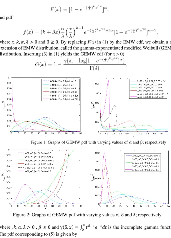
Figure 1: Graphs of GEMW pdf with varying values of α and β; respectively

Figure 2: Graphs of GEMW pdf with varying values of δ and λ; respectively

where , 𝑘, 𝛼, 𝜆 > 0 , 𝛽 ≥ 0 and γ(δ, 𝑥) = ∫ 𝑡₀𝑥 𝛿−1𝑒−𝑡𝑑𝑡is the incomplete gamma function. The pdf corresponding to (5) is given by

(5)

for 𝑥, 𝑘, 𝛼, 𝜆 > 0 and 𝛽 ≥ 0. A random variable X having density (6) is denoted by X~GEM

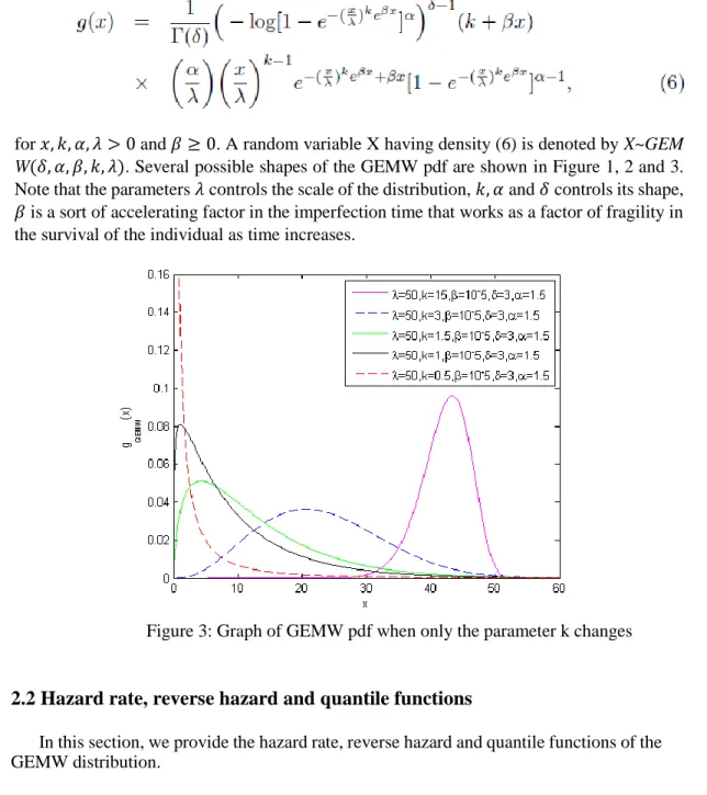
W(𝛿, 𝛼, 𝛽, 𝑘, 𝜆). Several possible shapes of the GEMW pdf are shown in Figure 1, 2 and 3.

Note that the parameters 𝜆 controls the scale of the distribution, 𝑘, 𝛼 and𝛿 controls its shape, 𝛽 is a sort of accelerating factor in the imperfection time that works as a factor of fragility in the survival of the individual as time increases.

Figure 3: Graph of GEMW pdf when only the parameter k changes

2.2 Hazard rate, reverse hazard and quantile functions

In this section, we provide the hazard rate, reverse hazard and quantile functions of the GEMW distribution.

2.2.1 Hazard rate and reverse hazard functions

Note that if X is a continuous random variable with cdf G(x); and pdf g(x); then the failure of hazard rate function (hrf), reverse hazard function (rhf) and mean residual life functions are given byℎ𝐺(𝑥) =

𝑔(𝑥) 𝐺̅(𝑥), 𝜏𝐺(𝑥) = 𝑔(𝑥) G(x); and𝛿𝐺(𝑥) = ∫ 𝐺̅(𝑢)𝑑𝑢/𝐺̅(𝑢) ∞ 𝑥 ,

respectively. The functions ℎ𝐺(𝑥), 𝛿𝐺(𝑥), and 𝐺̅(𝑥) are equivalent. (Shaked and

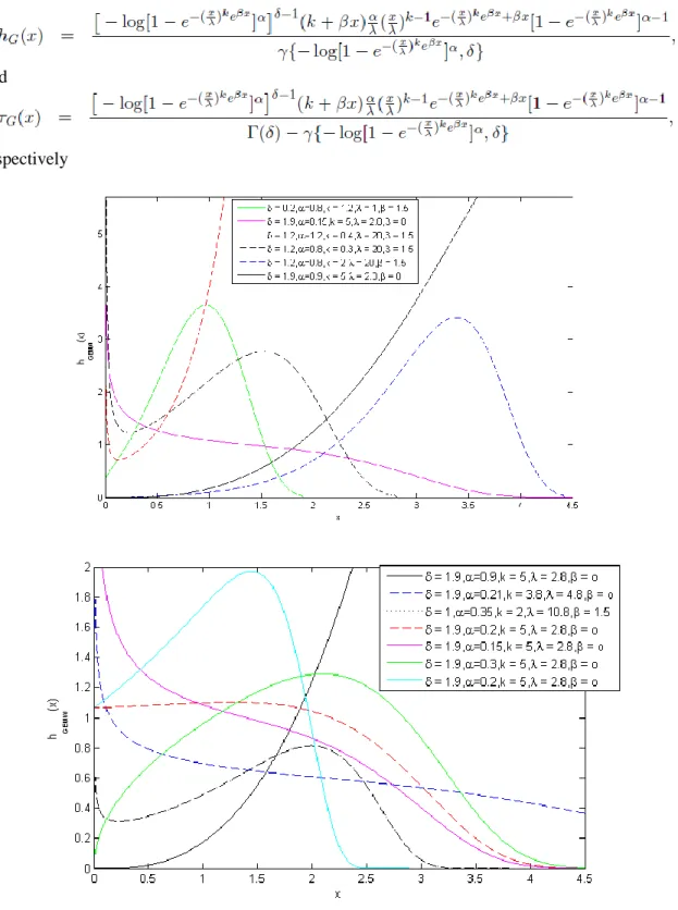
Shanthikumar, 1994). The hazard rate and reverse hazard rate functions of GEMW distribution are given by

(6)

and

respectively

Figure 4: Graphs of GEMW hazard function

Plots of hrf are presented in Figure 4. These plots show various shapes including monotonically decreasing, monotonically increasing, unimodal and bathtub shapes for different combinations of the values of the parameters. This flexibility makes the GEMW hrf

(7)

suitable for monotonic and non-monotonic empirical hazard behaviors which are more likely to be the case in real life situations.

The density and hazard functions can exhibit different behavior depending on the values of the parameters when chosen to be positive, as shown in these plots. However, it is hard to analyze the shape of both the density and hazard function due to their complicated forms.

2.2.2 Quantile function

We can know more about this model by expanding the density function and analyzing the quantile function. The GEMW quantile function can be obtained by inverting 𝐺̅(𝑥) = 1 − 𝑢, where 𝐺(𝑥) = 𝑢 and

and the inverse incomplete gamma function can be implemented by using numerical methods. Consequently, random number can be generated based on (8).

2.3 Expansion of the GEMW Density Function

Consider the series − log(1 − 𝑦) = ∑∞0 𝑦_𝑖+1𝑖+1 , where 0 < 𝑦 < 1 , and y = 𝑒−(

𝑥 𝜆)

𝑘_𝑒𝛽𝑥

. The GEMW distribution can be written as

Note that: Next , let 𝑎𝑠= 1 𝑠+2 , then (∑ 𝑎𝑠𝑦 𝑠₎ ∞ 𝑠=0 𝑚= ∑∞𝑠=0𝑏𝑠, 𝑦𝑚 𝑠 where

(8)

where 𝑓𝑀𝑊(𝑥) = 𝑓(𝑥; 𝑘, 𝛽, 𝜆𝑀𝑊)denotes the pdf of the modified Weibull distribution (Lai et al., 2003) with 𝜆𝑀𝑊 = 𝜆 (𝑟+𝑚+𝑠+𝛿) 1 𝑘

> 0. To simplify the notation, one can define 𝑉 = {(𝑚, 𝑠, 𝑟) ∈ 𝒁+𝟑} as an index set and the weights w𝑣 =(−1)

𝑟_𝛼𝛿 Γ(𝛿) ( 𝛿−1 𝑚 )( 𝛼−1 𝑟 ) 𝑏𝑠,𝑚 𝑟+𝑚+𝑠+𝛿, for 𝑣 ∈

𝑉. Therefore, the GEMW pdf can be written as

Equation (13) shows that the GEMW density is indeed a linear combination of modified Weibull distribution. Hence, most of its mathematical properties can be immediately obtained from those of the modified Weibull distribution. For the convergence of equations (12) and (13), as well elsewhere in this paper, note that for > 0;

so that

is convergent if and only if 0 < (𝑦 ∑∞𝑘=0_𝑘+2𝑦𝑘)𝑘< 1 ∀ 𝑦 ∈ (0,1),since 0 < y = 𝑒−(

𝑥 𝜆) 𝑘_𝑒𝛽𝑥 < 1,𝑥 > 0, 𝜆, 𝑘 > 0, and β ≥ 0 . Now , 0 < 𝑦 ∑∞𝑘=0_𝑘+2𝑦𝑘 = − log(1−y) y − 1 , so we must have 0 < −log(1−y)

y − 1 < 1 . This leads to 1 − y > exp (−2y) , and on the other hand

exp(−y) = ∑∞𝑘=0(−1)_𝑘!𝑘𝑦𝑘> 1 − y. Thus , we have the system of inequalities 1 − y >

exp (−2y) and exp(−y) > 1 − y , which is statisfied ∀y ∈ (0,0.7968).

2.4 Some Sub-models

In this section, some sub-models of the GEMW distribution are presented. The GEMW distribution contains several special sub-models that are well known distributions. When β = 0, we obtain

which is the gamma-exponentiated Weibull (GEW) distribution, given by Pinho et al. (2012). The GEW distribution has several special cases as its sub-models. For instance, = 1 leads to the exponentiated Weibull (EW) distribution (Gupta and Kundu, 2001), with a pdf:

(9)

When α = 𝑘 = 1 , EW distribution has the exponential distribution (Gupta and Kundu, 2001) as a sub-model with a pdf

By setting k = 1; EW distribution leads to the exponentiated exponential (EE) with a pdf

Let 𝛼 = 1, from EW distribution we can also obtain Weibull distribution (Weibull, 1951) whose pdf is given by

When 𝛽 = 0 , 𝛼 = 1and 𝛽 = 0, 𝛼 = 𝑘 = 1 , the gamma-Weibull (GW) (Pinho et al., 2012) with a pdf

and gamma-exponential (GE) (Pinho et al., 2012) distributions with a pdf

are obtained, respectively. The gamma-exponentiated exponential (GEE) distri-bution follows from 𝛽 = 0and k = 1, whose pdf is given by

Moreover, when 𝛽 = 0, 𝑘 = 2 𝑎𝑛𝑑 𝛽 = 0, 𝑘 = 2, 𝛼 = 1we obtain gamma-exponentiated Rayleigh (GER) (Ristic and Balakrishnan, 2011) distribution with a pdf

and gamma-Rayleigh (GR) distribution (Ristic and Balakrishnan, 2011) with a pdf

respectively.

When𝛽 ≠ 0 , by setting 𝛼 = 𝛿 = 1, we obtain the modified Weibull distribution (MW)

(10)

For 𝑘 = 0 , α = 1 and 𝑘 = 0 , δ = α = 1, GEMW gives gamma-extreme value (GEV) (Coles, 2001) and extreme value (EV) (Coles, 2001) distributions, with pdfs

and

respectively. One can also obtain gamma-modified Weibull (GMW) distribution by letting

α = 1 in GEMW distribution, the corresponding pdf of GMW is:

which is a new distribution.

3.

Moments, moment generating and characteristic functions

In this section, the moments, moment generating function and characteristic function of the GEMW distribution are presented. Let Z be a random variable with a density function

g(z), as in equation (6) and X be a random variable with modified Weibull density function 𝑓𝑀𝑊(𝑥).

3.1 Moments

As mention earlier in section 2.3, the GEMW distribution is a linear combination of modified Weibull distribution. Recall the general results for the beta-modi ed Weibull (BMW) distribution given by Nadarajah et al. (2011). Let 𝑌~𝐵𝑀𝑊(𝑎, 𝑏, 𝛼, 𝛾, 𝜆) with pdf

where 𝑎, 𝑏, α > 0 and γ, λ ≥ 0 . Note that 𝑓𝑀𝑊(𝑥) is a sub-model of BMW distribution

(Silva et al., 2010) with the parameters:

Using the moments of BMW distribution, the moments of the MW distribution (Nadarajah et al., 2011) are as follow:

(11)

where 𝐼1(𝑗, 𝑡), 𝑤𝑗 and 𝑎𝑗 given by

and

respectively.

There is also another relatively simpler form of the tth moment by using the Lambert W (.) function. We can get the following equation for 𝐼1(𝑗, 𝑡),

Substituting equation (18) in (14) gives a representation for moments of the MW (Lai et al., 2003) distribution in a relatively concise form with only a doubly infinite series. Thus, the moments of GEMW can be obtained from the moments above. Let 𝑍~𝐺𝐸𝑀𝑊(𝜆, 𝛿, 𝛼, 𝛽, 𝑘) , then E(Zt₎_{can be expressed in terms of the}_tth_{moments of the same baseline MW distribution,}

which is

where E(Xt) is defined by equation (14), and by substituting 𝐼1(𝑗, 𝑡) from equation (18), one

can also get another form of moments for GEMW distribution.

Conditional expectations are very useful for lifetime models, so it is very important to know E(𝑋𝑡|𝑋 > 𝑥), which is given by:

(12)

and 𝑤𝑗 𝑎𝑛𝑑 𝑎𝑗 are given by (16), (17) and Γ(𝑎, 𝑥) = ∫ 𝑦𝑎−1𝑒−𝑦𝑑𝑦 ∞

𝑥 .

Similarly, a relatively simpler representation for E(𝑋𝑡|𝑋 > 𝑥) can be obtained from equation (18),

3.2 Moment generating and characteristic functions

Let 𝑋~𝐺𝐸𝑀𝑊(𝜆, 𝛿, 𝛼, 𝛽, 𝑘), the moment generating function and characteristic function

of X are given by 𝑀(𝑡) = 𝐸(𝑒𝑡𝑥) and 𝜙(𝑡) = 𝐸(𝑒𝑖𝑡𝑥₎_{, respectively, where}_{𝑖 = √−1}_{. Note}

that 𝑀(𝑡) and 𝜙(𝑡) can be express as 𝑀(𝑡) = ∑ 𝑡𝑘

𝑘! ∞ 𝑘=0 𝐸(𝑋𝑘) and 𝜙(𝑡) = ∑ (𝑖𝑡)𝑘 𝑘! 𝐸(𝑋 𝑘₎ ∞ 𝑘=0 ,

where 𝐸(𝑋𝑘) is the given by equation (14). Nothing that, 𝑔(𝑥) can be expressed as an infinite weighted sum, we have

Where 𝑀𝑀𝑊(𝑡) is the moment generating function of the MW distribution, which is,

The corresponding characteristic function is

with

where 𝑤𝑗 is given by equation (16).

4.

Mean deviations, Bonferroni and Lorenz curves

In this section, mean deviations about the mean and the median, Bonferroni and Lorenz curves of the GEMW distribution are represented.

4.1 Mean deviations

Let 𝑋~𝐺𝐸𝑀𝑊(𝛿, 𝛼, 𝛽, 𝑘, 𝜆), the mean deviation about the mean and the mean deviation

about the median are defined by 𝛿1(𝑋) = ∫ |𝑥 − 𝑢|𝑔(𝑥)𝑑𝑥 ∞

0 , and 𝛿2(𝑋) = ∫ |𝑥 − ∞ 0

(13)

𝑀|𝑔(𝑥)𝑑𝑥, respectively, where μ = E(X) and 𝑀 = 𝑀𝑒𝑑𝑖𝑎𝑛(𝑋) denotes the median. The measures 𝛿1(𝑋) and 𝛿2(𝑋) can be calculated using the relationships

Recall that 𝑔(𝑥) = ∑𝜐∈𝑉𝜔𝑢𝑓𝑀𝑊(𝑥) , so that ∫ 𝑥𝑔(𝑥)𝑑𝑥 = ∞

𝜇 ∑𝜐∈𝑉𝜔𝑢𝐼3 and

∫ 𝑥𝑔(𝑥)𝑑𝑥 =_𝑀∞ ∑𝜐∈𝑉𝜔𝑢𝐼4 , where

and 𝜔𝑗 and 𝑎𝑗 are given by equation (16) and (17), respectively. It follows that

4.2 Bonferroni and Lorenz Curves

In this section, some inequality measures, namely Bonferroni and Lorenz curves are presented. These quantities have been applied to a wide variety of fields, such as studying of income and property in economics, reliability, demography, insurance and medicine.

For 𝑋~𝐺𝐸𝑀𝑊(𝛿, 𝛼, 𝛽, 𝑘, 𝜆), they are defined by

respectively, where 𝜇 = 𝐸(𝑋) and q = 𝐺−1(𝑝) is obtained from equation (8). Using similar methods in deriving the moments, we can show that

(14)

and 𝜔𝑗 and 𝑎𝑗 are given by equation (16) and (17), respectively. We can reduce the curves in

equation (25) to

respectively.

5.

Order Statistics and Renyi Entropy

In this section, the distribution of the ith order statistic and Renyi entropy for the GEMW distribution are presented.

5.1 Order Statistics

Consider 𝑋1, … . . , 𝑋𝑛 i.i.d random variables distributed according to (2). The pdf of the

ith order statistic, say𝑋𝑖:𝑛, is given by

Using the binomial theorem, the pdf of ith order statistic can be written as

Applying the power series (see Gradshteyn and Ryzhik, 2000)

we have

Let 𝑐𝑚= (−1)𝑚

𝑚!(𝑚+𝛿) and use the result on a power series raised to a positive integer, as in

(15)

where 𝑑0,𝑛+𝑗−𝑖 = 𝑐0 (𝑛+𝑗−𝑖)

and 𝑑𝑚,𝑛+𝑗−𝑖= (𝑚𝑐0)−1∑𝑚𝑙=1[(𝑛 + 𝑗 − 𝑖)𝑙 − 𝑚 +

𝑙] 𝑐𝑙𝑑𝑚−𝑙,𝑛+𝑗−𝑖. Replacing 𝑔(𝑥) by the right hand side of (2), we obtain

where 𝑔𝛿(𝑛+𝑗−𝑖+1)+𝑚(𝑥) denotes the GEMW with δ∗= δ(𝑛 + 𝑗 − 𝑖 + 1) + 𝑚 > 0 .

Consequently, 𝑔𝑖:𝑛(𝑥) is a linear combination of modified Weibull densities. This is very

useful result since we can derive properties of the order statistics of the GEMW distribution from those of modified Weibull distribution. For instance, we can obtain

where 𝐼1(𝑙, 𝑡) is given by equation (15). These moments are used in areas such as quality

control, reliability and insurance, for prediction of future failure times from a set of past failures.

5.2 Renyi Entropy

Renyi entropy is defined by

where 𝑣 > 0 and 𝑣 ≠ 1. Raising equation (6) to the power and using the similar expansion in section 2, we obtain

where 𝜆∗∗=

𝜆

(𝛿𝑣+𝑚+𝑠+𝑟)1/𝑘> 0 and 𝑏𝑠,𝑚 is given by equation (11). Consequently Renyi

(16)

(29) where 𝜔𝑗 and 𝑎𝑗 are given by equation (16) and (17), and Γ(a) = ∫ 𝑦𝑎−1𝑒−𝑦

∞

0 𝑑𝑦.

6.

Estimation of Parameters

Let 𝑋~𝐺𝐸𝑀𝑊(𝛿, 𝛼, 𝛽, 𝑘, 𝜆) and Δ = (𝛿, 𝛼, 𝛽, 𝑘, 𝜆)𝑇 be the parameter vector. The

log-likelihood for a single observation 𝑥 of X is given by

The first derivative of the log-likelihood function with respect to the parameters Δ = (𝛿, 𝛼, 𝛽, 𝑘, 𝜆)𝑇 are given by

(17)

The total log-likelihood function based on a random sample of n observations:{𝑥1, 𝑥2, … … 𝑥𝑛} drawn from the GEMW distribution is given by ℓ∗= 𝐿(Δ) =

∑𝑛𝑖=1ℓ𝑖(Δ), where ℓ𝑖(Δ), 𝑖 = 1,2, … … , n is given by equation (30). The equations obtained

by setting the above partial derivatives to zero are not in closed form and the values of the parameters α, β, θ, λ, δ must be found by using iterative methods. The maximum likelihood estimates of the parameters, denoted by Δ̂ is obtained by solving the nonlinear equation (𝜕ℓ_𝜕𝛼∗,𝜕ℓ_𝜕𝛽∗,𝜕ℓ_𝜕𝑘∗,𝜕ℓ_𝜕𝜆∗,𝜕ℓ_𝜕𝛿∗)T= 0 , using a numerical method such as Newton-Raphson procedure. We maximize the likelihood function using NLmixed in SAS as well as the function nlm in R (2011). These functions were applied and executed for wide range of initial values. This process often results or lead to more than one maximum, however, in these cases, we take the MLEs corresponding to the largest value of the maxima. In a few cases, no maximum was identified for the selected initial values. In these cases, a new initial value was tried in order to obtain a maximum.

The issues dealing with the existence and uniqueness of the MLEs are theo-retical interest and has been studied by several authors for di erent distributions including Seregin (2010), Santos Silva and Tenreyro (2010), Zhou (2009), and Xia et al. (2009). We hope to investigate this problem or issue for the GEMW distribution in the future.

Let Δ̂ = (α̂, β̂, k̂, λ̂, δ̂) be the maximum likelihood estimate of Δ = (α, β, k, λ, δ) Under the usual regularity conditions and that the parameters are in the inte-rior of the parameter space, but not on the boundary, (Ferguson, 1996) we have:

√𝑛(∆̂ − ∆)→ 𝑁𝑑 5(0, 𝐼−1(∆)), where 𝐼(∆) is the expected Fisher information matrix. The

asymptotic behavior is still valid if 𝐼(∆) is replaced by the observed information matrix evaluated at ∆̂ , that is J(∆̂). Elements of the observed information matrix are given in the Appendix. The multivariate normal distribution 𝑁5(0, 𝐽(∆̂)−1), where the mean vector 0 = (0,

0, 0, 0, 0)T , can be used to construct confidence intervals and confidence regions for the individual model parameters and for the survival and hazard rate functions. That is, the approximate 100(1 − η)% two-sided confidence intervals for α, β, k λ, and δ are given by:

and 𝛿̂ ± 𝑍𝜂 2

√𝐼_𝛿𝛿−1_(∆̂)_{, respectively, where}_𝐼

𝛼𝛼−1(∆̂), 𝐼𝛽𝛽−1(∆̂), 𝐼𝑘𝑘−1(∆̂), 𝐼𝜆𝜆−1(∆̂) and 𝐼𝛿𝛿−1(∆̂) are the

diagonal elements of 𝐼𝑛−1(∆̂) = (𝑛𝐼(∆̂))−1, and 𝑍𝜂

2 is the upper

𝜂𝑡ℎ

2 percentile od a standard

normal distribution.

The maximum likelihood estimates (MLEs) of the GEMW parameters α, β, θ, λ, and δ are computed by maximizing the objective function via the subroutine NLmixed in SAS. The estimated values of the parameters (standard error in parenthesis), -2log-likelihood statistic, Akaike Information Criterion, AIC = 2p− 2 ln(L), Bayesian Information Criterion, BIC = p ln(n) − 2 ln(L), and Consistent Akaike Information Criterion, AICC = AIC +2 𝑝(𝑝+1)_{𝑛−𝑝−1} , where L = L(∆̂ ) is the value of the likelihood function evaluated at the parameter estimates, n is the

(18)

number of observations, and p is the number of estimated parameters, and Kolmogorov-Smirnov (KS) statistic are presented in Tables 2 and 3.

In order to compare the models, we use the criteria stated above. Note that for the value of the log-likelihood function at its maximum (L(∆̂ )), larger value is good and preferred, and for the Kolmogorov-Smirnov test statistic (K-S), smaller value is preferred. GEMW distribution is fitted to the data sets and these fits are compared to the fits using the Exponential, Weibull, EE, GE, GEE, GW, EW, MW, GEW and GMW distributions.

We can use the likelihood ratio (LR) test to compare the fit of the GEMW distribution with its sub-models for a given data set. For example, to test λ = δ = 1, the LR statistic is 𝜔 = 2[𝑙𝑛 (𝐿(𝛼̂, 𝛽̂, 𝑘̂. 𝜆̂. 𝛿̂)) − 𝑙𝑛 (𝐿(𝛼̃, 𝛽̃, 𝑘̃, 1,1))], where α̂, β̂, k̂. λ̂ and δ̂, are the unrestricted estimates, and 𝛼̃, 𝛽̃, and 𝑘̃ are the restricted estimates. The LR test rejects the null hypothesis ifω > χ𝜖2, where χ𝜖2 denote the upper 100s% point of the χ2 distribution with 2 degrees of

freedom.

7.

Applications

In this section, we present two examples to illustrate the flexibility of the GEMW distribution and its sub-models for data modeling.

The first data consists of the lifetimes of n = 50 devices given by Aarset (1987). It is known to have a bathtub-shaped hazard function thus been widely studied. The dataset are: 0.1 0.2 1.0 1.0 1.0 1.0 1.0 2.0 3.0 6.0 7.0 11.0 12.0 18.0 18.0 18.0 18.0 18.0 21.0 32.0 36.0 40.0 45.0 46.0 47.0 50.0 55.0 60.0 63.0 63.0 67.0 67.0 67.0 67.0 72.0 75.0 79.0 82.0 82.0 83.0 84.0 84.0 84.0 85.0 85.0 85.0 85.0 85.0 86.0 86.0.

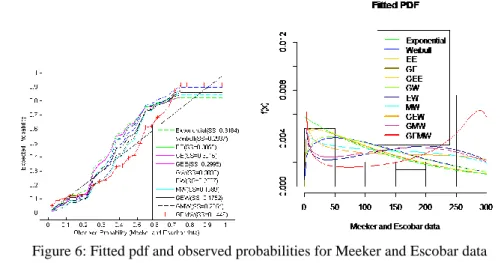
The second data gives failure and running times of a sample of n = 30 devices given by Meeker and Escobar (1998). This data has a bathtub shaped hazard function and are given by: 2 10 13 23 23 28 30 65 80 88 106 143 147 173 181 212 245 247 261 266 275 293 300 300 300 300 300 300 300 300.

Some descriptive statistics of these two data sets are given in Table 1.

Table 1: GEMW Descriptive Statistics of Application Data Sets

Data n Mean Media

n Minimu m Maximu m Varianc e SD Aarset 50 45.686 48.5 0.1 86.0 1078.2 32.8352 Meeke r 30 177.03 196.5 2 300 13223 114.991 3

Estimates of the parameters of GEMW distribution (standard error in parentheses), Akaike Information Criterion (AIC), Consistent Akaike Information Criterion (AICC), Bayesian Information Criterion (BIC) and Kolmogorov-Smirnov (KS) statistic are given in Table 2 for the first data set and in Table 3 for the second data set. The estimated covariance matrix for the GEMW distribution (Aarset Data) is given by

[ 208.87 −40.6120 −40.6120 0.08240 0.1575 3.3190 2.3599 −0.00033 −0.00641 −0.00453 0.1575 −0.00033 3.3190 2.3599 −0.00641 −0.00453 0.000237 0.001232 −0.0003 0.001232 −0.00003 0.01139 −0.0006 −0.0006 0.000294 ]

(19)

The 95% asymptotic confidence intervals for the GEMW model (Aarset Data) parameters are: α ∈ (0.01279, 0.07463), β ∈ (0.05552, 0.1244), δ∈ (0.1628, 0.5915), k∈ (3.9043, 5.0574), and λ∈ (317.7468, 374.2732), respectively.

(20)

Table 2: GEMW Estimation for Aarset data

Model

α

β

λ

k

δ

-2 Log Likelihood AIC BIC AICC KS

SS

Exponential

1

0

45.6858

1

482.2

484.2 486.1 484.3 0.1911 0.5190

-

(6.4609)

-

Weibull

1

0

44.9125

0.9490

1

482.0

486.0 489.8 486.3 0.1928 0.5289

-

(6.9451) (0.1196)

-

EE

0.7798

0

53.4739

1

480.0

484.0 487.8 484.2 0.2042 0.5634

(10.3680)

-

(0.1351)

-

GE

1

0

70.2848

1

1.3798

481.6

485.6 489.4 485.8 0.1981 0.5469

-

(40.4183)

-

(0.5253)

GEE

0.3148

0

7.0083

1

0.1403

477.2

483.2 488.9 483.7 0.1911 0.4920

(0.2004)

-

(7.8173)

-

(0.1521)

GW

1

0

83.0358

1.0597 1.5605

481.5

487.5 493.2 488.0 0.1974 0.5492

-

(12.9968) (0.1425) (0.3661)

EW

0.1275

0

91.0063

5.4117

1

457.0

463.0 468.7 465.3 0.2092 0.5679

(0.01843)

-

(6.5188) (0.1637)

-

MW

1

0.02332 2487.20

0.3548

1

454.3

460.3 466.0 460.8 0.1337 0.2662

-

(0.002633) (1.107) (0.05343)

-

GEW

0.08204

0

82.8604

5.5040 0.6182

451.8

458.7 466.3 459.6 0.1353 0.2248

(0.00714)

-

(20.5673) (0.1289) (0.0145)

GMW

1

0.02165

1231.0

0.3955 1.0017

454.5

462.5 470.1 463.4 0.1418 0.2773

-

(0.003056) (0.000125) (0.1584) (0.4751)

GEMW

0.04371 0.08996

346.01

4.4809 0.3771

434.3

444.3 453.9 445.7 0.1292 0.1497

(0.01539) (0.01714) (14.452) (0.2870) (0.1067)

(21)

Table 3: GEMW Estimation for Meeker and Escobar data

Model α β λ k δ -2 Log Likelihood AIC BIC AICC KS SS Exponential 1 0 172.75 1 1 356.8 358.8 360.2 359.0 0.2061 0.3184 - - (32.0784) - - Weibull 1 0 182.77 1.2359 1 355.3 359.3 362.0 359.7 0.2105 0.2937 - - (28.5726) (0.2023) - EE 1.1280 0 160.55 1 1 356.6 360.6 363.3 361.0 0.2067 0.3055 (0.2710) - (36.5670) - - GE 1 0 119.99 1 0.7315 356.5 360.5 363.2 361.0 0.2047 0.3015 - - (40.4183) - (0.5253) GEE 1.1370 0 170.00 1 1.0471 356.6 362.6 366.7 363.5 0.2042 0.2995 (0.2004) - (7.8173) - (0.1521) GW 1 0 330.00 1.4291 1.7402 354.9 360.9 365.0 361.9 0.2145 0.3033 - - (6.8530) (0.4399) (1.4851) EW 0.1286 0 325.36 6.8594 1 341.7 347.7 351.8 348.7 0.2199 0.2807 (0.01843) - (6.5188) (0.1637) - MW 1 0.006861 5055.05 0.4662 1 343.9 349.9 354.0 350.8 0.1766 0.1989 - (0.001021) (0.00001) (0.09065) - GEW 0.1025 0 329.47 7.1874 0.8469 340.9 348.9 354.3 350.5 0.1784 0.1752 (0.04242) - (10.3241) (0.4325) (0.2146) GMW 1 0.005980 1786.00 0.5343 0.9143 344.1 352.1 357.6 353.8 0.1860 0.2054 - (0.003056) (0.000125) (0.1584) (0.4751) GEMW 0.04764 0.03328 1567.01 5.5337 0.4426 330.1 340.1 346.9 342.7 0.1587 0.1446 (0.02313) (0.002379) (0.000066) (0.1088) (0.1846)

(22)

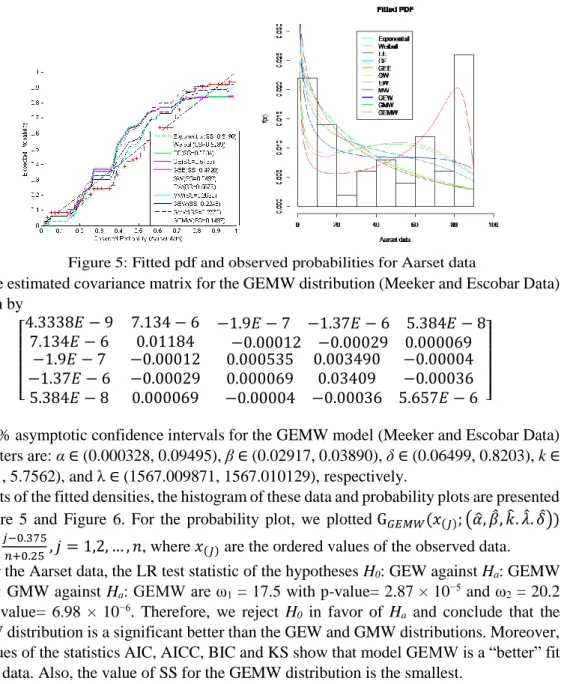
Figure 5: Fitted pdf and observed probabilities for Aarset data

The estimated covariance matrix for the GEMW distribution (Meeker and Escobar Data) is given by [ 4.3338𝐸 − 9 7.134 − 6 −1.9𝐸 − 7 −1.37𝐸 − 6 5.384𝐸 − 8 7.134𝐸 − 6 0.01184 −0.00012 −0.00029 0.000069 −1.9𝐸 − 7 −1.37𝐸 − 6 5.384𝐸 − 8 −0.00012 −0.00029 0.000069 0.000535 0.000069 −0.00004 0.003490 0.03409 −0.00036 −0.00004 −0.00036 5.657𝐸 − 6 ]

The 95% asymptotic confidence intervals for the GEMW model (Meeker and Escobar Data) parameters are: α ∈ (0.000328, 0.09495), β∈ (0.02917, 0.03890), δ∈ (0.06499, 0.8203), k∈ (5.3111, 5.7562), and λ ∈ (1567.009871, 1567.010129), respectively.

Plots of the fitted densities, the histogram of these data and probability plots are presented in Figure 5 and Figure 6. For the probability plot, we plotted G𝐺𝐸𝑀𝑊(𝑥(𝐽); (𝛼̂, 𝛽̂, 𝑘̂. 𝜆̂. 𝛿̂))

against 𝑗−0.375

𝑛+0.25 , 𝑗 = 1,2, … , 𝑛, where 𝑥(𝐽) are the ordered values of the observed data.

For the Aarset data, the LR test statistic of the hypotheses H0: GEW against Ha: GEMW

and H0: GMW against Ha: GEMW are ω1 = 17.5 with p-value= 2.87 × 10−5 and ω2 = 20.2

with p-value= 6.98 × 10−6. Therefore, we reject H0 in favor of Ha and conclude that the

GEMW distribution is a significant better than the GEW and GMW distributions. Moreover, the values of the statistics AIC, AICC, BIC and KS show that model GEMW is a “better” fit for this data. Also, the value of SS for the GEMW distribution is the smallest.

(23)

Figure 6: Fitted pdf and observed probabilities for Meeker and Escobar data

for the hypotheses H0: GEW against Ha: GEMW and H0: GMW against Ha: GEMW. The LR

test statistic of these hypothesis are ω3 = 10.8 with p-value= 0.001 and ω4 = 14 with p-value=

1.83 × 10−4, which implies that we should reject H0 in favor of Ha and conclude that the

GEMW distribution is a significant better fit for the Meeker and Escobar data. In addition, the values of the statistics AIC, AICC, BIC and KS clearly show that model GEMW is a “better” fit for this data. Furthermore, the value of SS for the GEMW distribution is the smallest.

8.

Concluding Remarks

A new class of distributions called the gamma-exponentiated or generalized modified Weibull (GEMW) distribution is proposed and studied. The GEMW distribution has several sub-models such as the GEW, EW, EE, GW, GE, GEE, GER, GR, MW, GEV, EV, GMW, Weibull, Rayleigh and exponential distributions as special cases. The density of this new class of distributions can be expressed as a linear combination of MW density functions. The GEMW distribution possesses hazard function with flexible behavior. We also obtain closed form expressions for the moments, distribution of order statistics and entropy. Maximum likelihood estimation technique is used to estimate the model parameters. Finally, the GEMW model is fitted to real data sets to illustrate the usefulness, flexibility and applicability of this class of distributions.

(24)

References

[1] Aarset, M.V. (1987). How to identify bathtub hazard rate, IEEE: Transactions

on Reliability, 36(1), 106-108.

[2] Bourguignon, M., Silva, R. B., Cordeiro, G. M. (2014). The Weibull-G family

of probability distributions, Journal of Data Science, 12, 53-68.

[3] Carrasco, M., Ortega, E.M., Cordeiro, G.M. (2008). A generalized modified

Weibull distribution for lifetime modeling, Computational Statistics and Data

Analysis, 53(2), 450-462.

[4] Coles, S. (2001). An introduction to statistical modeling of extreme values,

Springer Series in Statistics, London, Springer-Verlag.

[5] Eugene, N., Lee, C., Famoye, F. (2002). Beta-normal distribution and its appli-

cations, Communication in Statistics. Theory and Methods, 31, 497-512.

[6] Fergusen, T.A. (1996). A course in large sample theory, Chapman and Hall.

[7] Gupta, R.D., and Kundu, D. (1999). Generalized exponential distributions,

Australian and New Zealand Journal of Statistics, 41, 173-188.

[8] Gradshteyn, I.S., Ryzhik, I.M. (2000). Tables of integrals. Series and

Products,Academic Press: San Diego.

[9] Gupta, R.D., Kundu, D. (2001). Exponentiated exponential distribution: an

alternative to gamma and Weibull distributions, Biometrical Journal, 43,

117-130.

[10]Haupt, E., Schabe, H. (1992). A new model for a lifetime distribution with bathtub shaped failure rate, Microelectronics and Reliability, 32, 633-639.

[11]Hjorth, U. (1980). A reliability distribution with increasing, decreasing, con-

stant and bathtub failure rates, Technometrics, 22, 99-107.

[12]Jones, M.C. (2004). Families of distributions arising from distributions of order statistics, TEST, 13, 1-43.

[13]Kundu, D., Rakab, M.Z. (2005). Generalized Rayleigh distribution: different methods of estimation, Computational Statistics and Data Analysis, 49, 187-200.

[14]Lai, C.D., Xie, M., Murthy, D.N.P. (2003). A modified Weibull distribution,

IEEE Transactions on Reliability, 52, 33-37.

[15]Meeker, W.Q., Escobar, L.A. (1998). Statistical methods for reliability data,

(25)

[16]Merovci, F., Elbatal, I. (2015). A new generalization of exponentiated modified Weibull Distribution, Journal of Data Science, 13(2), 213-240.

[17]Nadarajah, S., Cordeiro, G.M., Ortega, E.M.M. (2011). General results for the

beta-modified Weibull distribution, Journal of Statistical Computation and

Simulation, 81(10), 1211-1232.

[18]Nadarajah, S., Kotz, S. (2006). The beta exponential distribution, Reliability

Engineering and System Safety, 91, 689-697.

[19]Nelson, W. (1982). Lifetime data analysis, Wiley, New York.

[20]Pham, H., Lai, C.D. (2007). On recent generalizations of the Weibull distribu-

tion, IEEE, Transaction on Reliability, 56, 454-458.

[21]Pinho, G.B., Cordeiro, G.M., Nobre, J.S. (2012). The gamma-exponentiated

Weibull distribution, Journal of Statistical Theory and Applications, 11(4), 379-395.

[22]R Development Core Team, (2011). A Language and Environment for Statistical

Computing, R Foundation for Statistical Computing, Vienna, Austria.

[23]Rajarshi, S., Rajarshi, M.B. (1988). Bathtub distributions: A review, Commu-

nications in Statistics-Theory and Methods, 17, 2521-2597.

[24]Risti´c, M.M., Balakrishnan, N. (2011). The gamma-exponentiated exponen-

tial distribution, Journal of Statistical Computation and Simulation, 82(8), 1191-1206.

[25]Shaked, M., Shanthikumar, J.G. (1994). Stochastic orders and their applications,

New York, Academic Press.

[26]Silva, G.O., Ortega, E.M.M., Cordeiro, G.M. (2010). The beta modified Weibull

distribution, Lifetime Data Analysis, 16, 409-430.

[27]Seregin, A. (2010). Uniqueness of the maximum likelihood estimator for k- monotone densities, Proceedings of the American Mathematical Society, 10(138), 4511-4515.

[28]Santos-Silva. J.M.C., Tenreyro, S. (2010). On the existence of maximum likeli-

hood estimates in Poisson regression, Economics Letters, 107, 310-312.

[29]Zhou, C. (2009). Existence and Consistency of the maximum likelihood estima-

tor for the extreme index, Journal of Multivariate Analysis, 100, 794-815.

[30]Xia, J., Mi, J., Zhou, Y.Y. (2009). On the existence and uniqueness of the maximum likelihood estimators of normal and log-normal population parameters with grouped data, Journal of Probability and Statistics, Article id

(26)

[31]Zografos, K., Balakrishnan, N. (2009). On families of beta and generalized

gamma-generated distribution and associated inference, Statistical Method-

ology, 6, 344-362.

[32]Weibull, W. (1951). Statistical distribution function of wide applicability, Jour-

(27)