Data Mining for Discrimination Discovery
SALVATORE RUGGIERI, DINO PEDRESCHI, FRANCO TURINI Dipartimento di Informatica, Universit`a di Pisa, Italy
In the context of civil rights law, discrimination refers to unfair or unequal treatment of people based on membership to a category or a minority, without regard to individual merit. Discrim-ination in credit, mortgage, insurance, labor market, and education has been investigated by researchers in economics and human sciences. With the advent of automatic decision support systems, such as credit scoring systems, the ease of data collection opens several challenges to data analysts for the fight against discrimination. In this paper, we introduce the problem of discovering discrimination through data mining in a dataset of historical decision records, taken by humans or by automatic systems. We formalize the processes of direct and indirect discrimina-tion discovery by modelling protected-by-law groups and contexts where discriminadiscrimina-tion occurs in a classification rule based syntax. Basically, classification rules extracted from the dataset allow for unveiling contexts of unlawful discrimination, where the degree of burden over protected-by-law groups is formalized by an extension of the lift measure of a classification rule. In direct discrimination, the extracted rules can be directly mined in search of discriminatory contexts. In indirect discrimination, the mining process needs some background knowledge as a further input, e.g., census data, that combined with the extracted rules might allow for unveiling contexts of discriminatory decisions. A strategy adopted for combining extracted classification rules with background knowledge is called an inference model. In this paper, we propose two inference mod-els and provide automatic procedures for their implementation. An empirical assessment of our results is provided on the German credit dataset and on the PKDD Discovery Challenge 1999 financial dataset.
Categories and Subject Descriptors: H.2.8 [Database Applications]: Data Mining General Terms: Algorithms, Economics, Legal Aspects
Additional Key Words and Phrases: Discrimination, Classification Rules
1. INTRODUCTION
The worddiscrimination originates from the Latin discriminare, which means to “distinguish between”. In social sense, however, discrimination refers specifically to an action based on prejudice resulting in unfair treatment of people on the basis of their membership to a category, without regard to individual merit. As an ex-ample, U.S. federal laws [U.S. Federal Legislation 2009] prohibit discrimination on the basis of race, color, religion, nationality, sex, marital status, age and pregnancy in a number of settings, including: credit/insurance scoring (Equal Credit
Oppor-Corresponding author’s address: S. Ruggieri, Dipartimento di Informatica, Universit`a di Pisa, L.go B. Pontecorvo 3, 56127 Pisa (Italy). e-mail: [email protected]. A preliminary version of this paper appeared inProc. of KDD 2008[Pedreschi et al. 2008]
Permission to make digital/hard copy of all or part of this material without fee for personal or classroom use provided that the copies are not made or distributed for profit or commercial advantage, the ACM copyright/server notice, the title of the publication, and its date appear, and notice is given that copying is by permission of the ACM, Inc. To copy otherwise, to republish, to post on servers, or to redistribute to lists requires prior specific permission and/or a fee.
c
tunity Act); sale, rental, and financing of housing (Fair Housing Act); personnel selection and wages (Intentional Employment Discrimination Act, Equal Pay Act, Pregnancy Discrimination Act). Other U.S. federal laws exist on discrimination in public programs or activities, such as public accommodations, education, health care, academic programs, student services, nursing homes, adoptions, senior citizens centers, hospitals, transportation. Several authorities (regulation boards, consumer advisory councils, commissions) are settled to monitor discrimination compliances in U.S., European Union and many other countries.
Concerning the research side, the issue of discrimination in credit, mortgage, in-surance, labor market, education and other human activities has attracted much interest of researchers in economics and human sciences since late ’50s, when a theory on the economics of discrimination was proposed [Becker 1957]. The litera-ture in those research fields has given evidence of unfair treatment in racial profiling and redlining [Squires 2003], mortgage discrimination [LaCour-Little 1999], person-nel selection discrimination [Holzer et al. 2004; Kaye and Aickin 1992], and wages discrimination [Kuhn 1987].
The importance of data collection and data analysis for the fight against dis-crimination is emphasized in legal studies promoted by the European Commission [Makkonen 2007]. The possibility of accessing to historical data concerning deci-sions made in socially-sensitive tasks is the starting point for discovering discrimi-nation. However, if available decision records accessible for inspection increase, the data available to decision makers for drawing their decisions increase at a much higher pace, together with ever more intelligent decision support systems, capable of assisting the decision process, and sometimes to automate such process entirely. As a result, the actual discovery of discriminatory situations and practices, hidden in the decision records under analysis, may reveal an extremely difficult task. The reason for this difficulty is twofold.
First, personal data in decision records are highly dimensional, i.e., character-ized by many multi-valued variables: as a consequence, a huge number of possible contexts may, or may not, be the theater for discrimination. To see this point, consider the case of gender discrimination in credit approval: although an analyst may observe that no discrimination occurs in general, i.e., when considering the whole available decision records, it may turn out that it is extremely difficult for aged women to obtain car loans. Many small or large niches may exist that conceal discrimination, and therefore all possible specific situations should be considered as candidates, consisting of all possible combinations of variables and variable values: personal data, demographics, social, economic and cultural indicators, etc. Clearly, the anti-discrimination analyst is faced with a huge range of possibilities, which make her work hard: albeit the task of checking some known suspicious situations can be conducted using available statistical methods, the task of discovering niches of discrimination in the data is unsupported.
The second source of complexity is indirect discrimination: often, the feature that may be object of discrimination, e.g., the race or ethnicity, is not directly recorded in the data. Nevertheless, racial discrimination may be equally hidden in the data, for instance in the case where ared-lining practice is adopted: people living in a certain neighborhood get frequently credit denial, and by demographic data we can
learn that most of people living in that neighborhood belong to the same ethnic minority. Once again, the anti-discrimination analyst is faced with a large space of possibly discriminatory situations: how can she highlight all interesting discrimina-tory situations that emerge from the data, both directly and in combination with further background knowledge in her possession (e.g., census data)?
The goal of our research is precisely to address the problem of discovering discrim-ination in historical decision records by means of data mining techniques. Generally, data mining is perceived as an enemy of fair treatment and as a possible source of discrimination, and certainly this may be the case, as we discuss below. Nonethe-less, we will show that data mining can also be fruitfully put at work as a powerful aid to the anti-discrimination analyst, capable of automatically discovering the pat-terns of discrimination that emerge from the available data with stronger evidence. Traditionally, classification models are constructed on the basis of historical data exactly with the purpose of discrimination in the original Latin sense: i.e., dis-tinguishing between elements of different classes, in order to unveil the reasons of class membership, or to predict it for unclassified samples. In either cases, clas-sification models can be adopted as a support to decision making, clearly also in socially sensitive tasks. For instance, a large body of literature [Baesens et al. 2003; Hand 2001; Hand and Henley 1997; Thomas 2000; Viaene et al. 2001; Vojtek and Koˇcenda 2006] refers to classification models as the basis of scoring systems to predict the reliability of a mortgage/credit card debtor or the risk of taking up an insurance. Furthermore, data mining screening systems have recently been pro-posed for personnel selection [Chien and Chen 2008]. While classification models used for decision support can potentially guarantee less arbitrary decisions, can they be discriminating in the social, negative sense? The answer is clearly yes: it is evident that relying on mined models for decision making does not put ourselves on the safe side. Rather dangerously, learning from historical data may mean to discover traditional prejudices that are endemic in reality, and to assign to such practices the status of general rules, maybe unconsciously, as these rules can be deeply hidden within a classifier. For instance, if it is a current malpractice to deny pregnant women the access to certain job positions, there is a high chance to find a strong association in the historical data between pregnancy and access denial, and therefore we run the risk of learning discriminatory decisions. This use of classifica-tion and predicclassifica-tion models may therefore exacerbate the risks of discriminaclassifica-tion in socially-sensitive decision making. However, as we show in this paper, data mining also provides a powerful tool for discovering discrimination, both in the records of decisions taken by human decision makers, and in the recommendations provided by classification models, or any combinations thereof.
In this paper, we tackle the problem of discovering discrimination within a rule-based setting, by introducing the notion of discriminatory classification rules, as a criterion to identify and analyse the potential risk of discrimination. By mining all discriminatory classification rules from a dataset of historical decision records, we offer a sound and practical method to discover niches of direct and indirect discrimination hidden in the data, as well as a criterion to measure discrimination in any such contexts. This extends our KDD 2008 paper [Pedreschi et al. 2008] in many respects: besides providing a detailed account of the theoretical aspects,
under a conservative extension of the syntax of frequent itemsets, it offers: a new perspective on the problem of discrimination discovery; an extended framework for anti-discrimination analysis, including a new inference model based on negated items; a more in depth experimental assessment; and a complexity evaluation of the algorithms proposed. A precise account of the differences between this paper and the KDD 2008 paper is provided in the Related Work section.
1.1 Plan of the Paper
The paper is organized as follows. In Sec. 2 we present a scenario for the analysis of direct and indirect discrimination. In Sec. 3 some standard notions on association and classification rules are recalled, and the measure of extended lift is introduced. In Sec. 4, we formalize the scenario of Sec. 2 by introducing the notions of α -protective andα-discriminatory classification rules, whereαis a user threshold on the acceptable level of discrimination. The two notions are refined for binary classes to strongα-protection and strongα-discrimination. Direct discrimination checking is presented in Sec. 5, with experimentation on the German credit dataset. Indirect discrimination is considered in Sec. 6 and Sec. 7, where background knowledge is adopted in two inference models. Experimentation on the German credit dataset is reported as well. Further experimentation on the Discovery Challenge 1999 financial dataset is presented in Sec. 8. Related work is reported in Sec. 9, while Sec. 10 summarizes the contribution of the paper. All proofs of theorems are reported in the Appendix A, where a conservative extension of the standard notions of association and classification rules is introduced. Computational complexity in time and space of the procedures presented in this paper are discussed in the Appendix B.
2. DISCRIMINATION ANALYSIS
The basic problem we are addressing can be stated as follows. Given: —a dataset of historical decision records,
—a set of potentially discriminated groups, —and a criterion of unlawful discrimination;
find all pairs consisting of a subset of the decision records, called a context, and a potentially discriminated group within the context for which the criterion of unlaw-ful discrimination hold. In this section, we describe those elements and the process of discrimination analysis in a framework based on itemsets, and on classification rules extracted from the dataset. In the next section, the various elements are formalized and the process is automated.
2.1 Potentially Discriminatory Itemsets
The first natural attempt to formally model potentially discriminated groups is to specify a set of selected attribute values (or, at an extreme, an attribute as a whole) as potentially discriminatory: examples include female gender, ethnic minority, low-level job, specific age range. However, this simple approach is flawed, in that discrimination may be the result of several joint characteristics that are not discriminatory in isolation. For instance, black cats crossing your path are typically discriminated as signs of bad luck, but no superstition is independently associated
to being a cat, being black or crossing a path. In other words, the condition that describes a (minority) population that may be the object of discrimination should be stated as a conjunction of attributes values: pregnant women, minority ethnicity in disadvantaged neighborhoods, senior people in weak economic conditions, and so on. Coherently, we qualify as potentially discriminatory (PD) some selected itemsets, not necessarily single items nor whole attributes. Two consequences of this approach should be considered. First, single PD items or attributes are just a particular case in this more general setting. Second, PD itemsets are closed under intersection: the conjunction of two PD itemsets is a PD itemset as well, coherently with the intuition that the intersection of two disadvantaged minorities is a, possibly empty, smaller (even more disadvantaged) minority as well. In our approach, we assume that the analyst interested in studying discrimination compiles a list of PD itemsets with reference to attribute-value pairs that are present either in the data, or in her background knowledge, or in both.
2.2 Modelling the Process of Direct Discrimination Analysis
Discrimination has been identified in law and social study literature as eitherdirect
or indirect (sometimes called systematic) [U.K. Legislation 2009; Australian Leg-islation 2009; Hunter 1992; Knopff 1986]. Direct discrimination consists of rules or procedures that explicitly impose “disproportionate burdens” on minority or disadvantaged groups.
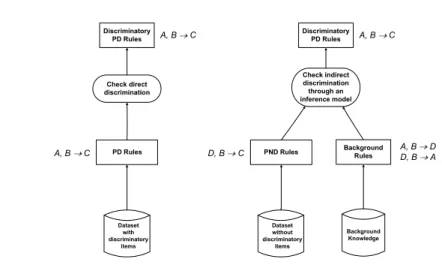
We unveil direct discrimination through the extraction from the dataset of his-torical decision records of potentially discriminatory (PD) rules defined as classi-fication rules A,B → C that contain potentially discriminatory itemsets A in their premises. A PD rule does not necessarily provide evidence of discriminatory actions. In order to measure the “disproportionate burdens” that a rule imposes, the notion of α-protection is introduced as a measure of the discrimination power of a PD classification rule. The idea is to define such a measure as the relative gain in confidence of the rule due to the presence of the discriminatory itemsets. The α parameter is the key for unveiling the desired level of protection against discrimination or, in other words, for stating the boundary between lawful and un-lawful discrimination. PD classification rules are extracted (see Fig. 1 left) from a dataset containing potentially discriminatory itemsets. This is the case, for in-stance, wheninternal auditors,regulation authoritiesorconsumer advisor councils
want to discover:
—discrimination malpractices; or
—positive policies – or affirmative actions [Holzer and Neumark 2006], that tend to favor some disadvantaged categories;
that emerge from the historical decision records. They collect the dataset of past transactions and enrich it, if necessary, with potentially discriminatory itemsets in order to extract discriminatory PD classification rules.
2.3 Modelling the Process of Indirect Discrimination Analysis
Indirect discrimination consists of rules or procedures that, while not explicitly mentioning discriminatory attributes, intentionally or not impose the same dispro-portionate burdens. For instance, the information on a person’s race is typically not
Dataset without discriminatory items Background Rules Background Knowledge Check indirect discrimination through an inference model Discriminatory PD Rules PND Rules A, B D D, B A D, B C A, B C Dataset with discriminatory items Check direct discrimination Discriminatory PD Rules PD Rules A, B C A, B C
Fig. 1. Modelling the process of direct (left) and indirect (right) discrimination analysis.
available (unless the dataset has been explicitly enriched) or not even collectable. Still, the dataset may unveil discrimination against minority groups.
We unveil indirect discrimination through classification rules D,B → C that are potentially non-discriminatory (PND), i.e., that do not contain PD itemsets. They are extracted (see Fig. 1 right) from a dataset which may not contain PD itemsets. While apparently unrelated to discriminatory decisions, PND rules may unveil discrimination as well. As an example, assume that the PND rule “rarely give credit to persons from neighborhood 10451 from NYC” is extracted. This may be or may be not a redlining rule. In order to unveil its nature, we have to rely on additionalbackground knowledge. If we know that in NYC people from neigh-borhood 10451 are in majority black race, then using the rule above is like using the PD rule “rarely give credit to black-race persons from neighborhood 10451 of NYC”, which is definitively discriminatory. Summarizing, internal auditors, regula-tion authorities, and consumer advisory councils can unveil indirect discriminaregula-tion by identifying discriminatory PD rules through some deduction starting from PND rules and background knowledge. The deduction strategy is called here aninference model. In our framework, we assume that background knowledge takes the form of association rules relating a PND itemsetDto a potentially discriminatory itemset
Awithin the contextB, or, formally, rules of the formD,B → AandA,B → D. Examples of background knowledge include the one originating from publicly avail-able data (e.g., census data), from privately owned data (e.g., market surveys) or from experts or common sense (e.g., expert rules about customer behavior).
As a final note, this use case resembles the situation described in privacy-preserving data mining [Agrawal and Srikant 2000; Sweeney 2001], where an anonymized dataset coupled with external knowledge might allow for the inference of the iden-tity of individuals.
2.4 An Example of Direct and Indirect Discrimination Analysis
a. city=NYC b. race=black, city=NYC
==> class=bad ==> class=bad
-- conf:(0.25) -- conf:(0.75)
Rule(a)can be translated into the statement “people who live in NYC are assigned the bad credit class” 25% of times. Rule (b)concentrates on “black people from NYC”. In this case, the additional (discriminatory!) item in the premise increases the confidence of the rule up to 3 times! α-protection is intended to detect rules where such an increase is lower than a fixed thresholdα.
In direct discrimination, rules such as (a)and (b)above are extracted directly from the dataset of historical decision records. Given a thresholdα of lawful dis-crimination, all extracted PD rules, including(b), can be checked forα-protection (see Fig. 1 left). For instance, if the threshold α= 3 is fixed by the analyst, rule
(b)would be classified as discriminatory, i.e., as unveiling discriminatory decisions. Tackling indirect discrimination is more challenging. Continuing the example, consider the classification rule:
c. neighborhood=10451, city=NYC ==> class=bad
-- conf:(0.95)
extracted from a dataset where potentially discriminatory itemsets, such as
race=-black, are NOT present (see Fig. 1 right). Taken in isolation, rule (c) cannot
be considered discriminatory or not. Assume now to know from census data that people from neighborhood 10451 are in majority black, i.e., the following association rule holds:
d. neighborhood=10451, city=NYC ==> race=black
-- conf:(0.80)
Despite rule (c) contains no discriminatory item, it unveils the discriminatory decision of denying credit to a minority sub-group (black people) which has been “redlined” by its ZIP code. In other words, the PD rule:
e. race=black, neighborhood=10451, city=NYC ==> class=bad
can be inferred from (c) and (d), together with a lower bound of 94% for its confidence. Such a lower bound shows a disproportionate burden (94% / 25%, i.e., 3.7 times) over black people living in neighborhood 10451. We will show an inference model, stated as a formal theorem, that allows us to derive the lower boundα≥3.7 forα-protection of(e)starting from PND rules(a)and(c)and a lower bound on the confidence of the background rule(d).
3. BASIC DEFINITIONS AND REFERENCE DATASET 3.1 Association and Classification Rules
We recall the notions of itemsets, association rules and classification rules from standard definitions [Agrawal and Srikant 1994; Liu et al. 1998; Yin and Han 2003]. LetRbe a relation with attributesa1, . . . , an. A class attribute is a fixed attribute
c of the relation. An a-item is an expression a= v, wherea is an attribute and
v∈dom(a), the domain ofa. We assume thatdom(a) is finite for every attribute
a. A c-item is called a class item. An item is any a-item. Let I be the set of all items. A transaction is a subset ofI, with exactly onea-item for every attributea. A database of transactions, denoted byD, is a set of transactions. An itemset X
is a subset ofI. We denote by 2I the set of all itemsets. As usual in the literature,
we writeX,Y forX∪Y. For a transactionT, we say thatT verifiesXifX⊆T. The support of an itemsetXw.r.t. a non-empty transaction databaseDis the ratio of transactions inD verifyingX with respect to the total number of transactions:
suppD(X) = |{ T ∈ D | X⊆T }|/|D|, where | | is the cardinality operator. An
association rule is an expression X → Y, where X and Y are itemsets. X is called the premise(or the body) andY is called the consequence(or thehead) of the association rule. We say thatX → Yis aclassification ruleifYis a class item andXcontains no class item. We refer the reader to [Liu et al. 1998; Yin and Han 2003] for a discussion of the integration of classification and association rule mining. The support ofX → Yw.r.t.D is defined as: suppD(X → Y) =suppD(X,Y).
The confidence ofX → Y, defined whensuppD(X)>0, is:
confD(X → Y) =suppD(X,Y)/suppD(X).
Support and confidence range over [0,1]. We omit the subscripts in suppD() and
confD() when clear from the context. Since the seminal paper by Agrawal and
Srikant [1994], a number of well explored algorithms [Goethals 2009] have been de-signed in order to extractfrequentitemsets, i.e., itemsets with a specified minimum support, and valid association rules, i.e., rules with a specified minimum confidence. The proofs of the formal results presented in the paper suggested a conservative extension of the syntax of rules to boolean expressions over itemsets. The extension, reported in Appendix A.1, allows us to deal uniformly with negation and disjunction of itemsets. As a consequence of the improved expressive power of this language, the formal results of this paper directly extend to association and classification rules over over hierarchies [Srikant and Agrawal 1995] and negated itemsets [Wu et al. 2004].
3.2 Extended Lift
We introduce a key concept for our purposes.
Definition 3.1. [Extended lift] LetA,B → C be an association rule such that conf(B → C)>0. We define the extended lift of the rule with respect toB as:
conf(A,B → C)
conf(B → C) .
We call Bthe context, and B → C the base-rule.
Intuitively, the extended lift expresses the relative variation of confidence due to the addition of the extra itemset A in the premise of the base rule B → C. In general, the extended lift ranges over [0,∞[. However, if association rules with a minimum support ms >0 are considered, it ranges over [0,1/ms]. Similarly, if association rules with base-rules with a minimum confidencemc >0 are considered, it ranges over [0,1/mc]. The extended lift can be traced back to the well-known
measure oflift[Tan et al. 2004] (also known asinterest factor), defined as:
lif tD(A → C) =confD(A → C)/suppD(C).
The extended lift ofA,B → C with respect toBis equivalent tolif tB(A → C)
where B = {T ∈ D |B⊆T} is the set of transactions satisfying the context B. When B is empty, the extended lift reduces to the standard lift. We refer the reader to Appendix A.2 for proofs of these statements.
3.3 The German credit case study
Throughout the paper, we illustrate the notions introduced by analysing the public domain German credit dataset [Newman et al. 1998], consisting of 1000 transactions representing the good/bad credit class of bank account holders. The dataset include nominal (or discretized) attributes onpersonal properties: checking account status, duration, savings status, property magnitude, type of housing; on past/current credits and requested credit: credit history, credit request purpose, credit request amount, installment commitment, existing credits, other parties, other payment plan; onemployment status: job type, employment since, number of dependents, own telephone; and onpersonal attributes: personal status and gender, age, resident since, foreign worker.
4. MEASURING DISCRIMINATION 4.1 Discriminatory Itemsets and Rules
Our starting point consists of flagging at syntax level those itemsets which might potentially lead to discrimination in the sense explained in Section 2.1. A set of itemsetsI ⊆2I is downward closed if whenA
1∈ I andA2∈ I thenA1,A2∈ I.
Definition 4.1. [PD/PND itemset] A set of potentially discriminatory (PD) itemsets Id is any downward closed set. Itemsets in 2I \ Id are called potentially
non-discriminatory (PND).
Any itemsetXcan be uniquely split into a PD partAand a PND partB=X\A
by settingAto the largest subset ofXthat belongs toId1. A simple way of defining
PD itemsets is to take those that are built from a pre-defined set of items, that is to reduce to the case where the granularity of discrimination is at the level of items.
Example 4.2. For the German credit dataset, we fix Id = 2Id, where Id is
the set of the following (discriminatory) items: personal status=female
div/-sep/mar (female and not single), age=(52.6-inf) (senior people),
job=unemp/-unskilled non res(unskilled or unemployed non-resident), andforeign
worker=-yes (foreign workers). Notice that the PD part of an itemset X is now easily identifiable asX∩Id, and the PND part as X\Id.
It is worth noting that discriminatory items do not necessarily coincide with sensitive attributes with respect to pure privacy protection. For instance, gender is generally considered a non-sensitive attribute, whereas it can be discriminatory
1Notice thatAis univocally defined. If there were two maximalA
16=A2 subsets belonging to
Id, thenA1,A2 would belong toId as well sinceId is downward closed. But thenA1 or A2
in many decision contexts. Moreover, note that we use the adjective potentially
both for PD and PND itemsets. As we will discuss later on, also PND itemsets may unveil (indirect) discrimination. The notion of potential (non-)discrimination is now extended to rules.
Definition 4.3. [PD/PND classification rule] A classification ruleX → C is potentially discriminatory (PD) ifX=A,BwithAnon-empty PD itemset and B PND itemset. It is potentially non-discriminatory (PND) if Xis a PND itemset.
It is worth noting that PD rules can be either extracted from a dataset that contains PD itemsets or inferred as shown in Fig. 1 right. PND rules can be extracted from a dataset which may or may not contain PD itemsets.
Example 4.4. Consider Ex. 4.2, and the rules:
a. personal_status=female div/sep/mar savings_status=no known savings ==> class=bad
b. savings_status=no known savings ==> class=bad
(a)is a PD rule since its premise contains an item belonging toId. On the contrary, (b)is a PND rule. Notice that(b)is the base rule of(a)if we consider as context the PND part of its premise.
4.2 α-protection
We start concentrating on PD classification rules as the potential source of discrim-ination. In order to capture the idea of when a PD rule may lead to discrimination, we introduce the key concept ofα-protective classification rules.
Definition 4.5. [α-protection] Let c=A,B → Cbe a PD classification rule, whereA is a PD andB is a PND itemset.
For a given thresholdα≥0, we say thatc isα-protective if its extended lift with respect to Bis lower thanα. Otherwise,c isα-discriminatory.
In symbols, given:
γ=conf(A,B → C) δ=conf(B → C)>0, we writeelif t(γ, δ)< αas a shorthand for cbeing α-protective, where:
elif t(γ, δ) =γ/δ. Analogously,c isα-discriminatory ifelif t(γ, δ)≥α.
Intuitively, the definition assumes that the extended lift ofcw.r.t.Bis a measure of the degree of discrimination of A in the context B. α-protection states that the added (potentially discriminatory) information A increases the confidence of concluding an assertionCunder the base hypothesisBonly by an acceptable factor, bounded byα.
Example 4.6. Consider again Ex. 4.2. Fixα= 3 and consider the classification rules:
a. personal_status=female div/sep/mar savings_status=no known savings ==> class=bad
-- supp:(0.013) conf:(0.27) elift:(1.52) b. age=(52.6-inf)
personal_status=female div/sep/mar purpose=used car
==> class=bad
-- supp:(0.003) conf:(1) elift:(6.06)
Rule (a) can be translated as follows: with respect to people asking for credit whose saving status were not known, then the bad credit class was assigned in past to non-single women 52% more than the average. The support of the rule is 1.3%, its confidence 27%, and its extended lift 1.52. Hence, the rule isα-protective. Also, the confidence of the base rule:
savings status=no known savings ==> class=bad
is 0.27/1.52 = 17.8%. Rule(b)states that senior non-single women that want to buy a used car were assigned the bad credit class with a probability more than 6 times the average one for those that asked credit for the same purpose. The support of the rule is 0.3%, its confidence 100%, and its extended lift 6.06. Hence the rule isα-discriminatory. Finally, note that the confidence of the base rule:
purpose=used car ==> class=bad
is 1/6.06 = 16.5%.
A general principle in discrimination laws is to consider group representation [Knopff 1986] as a quantitative measure of the qualitative requirement that people in a group are treated “less favorably” [European Union Legislation 2009; U.K. Legislation 2009] than others, or such that “a higher proportion of people without the attribute comply or are able to comply” [Australian Legislation 2009] to a qualifying criteria. We observe that (see Lemma A.9):
elif t(γ, δ) = conf(B,C → A)
conf(B → A) ,
namely the extended lift can be defined as the ratio between the proportion of the disadvantaged group A in context B obtaining the benefit C over the over-all proportion of A in B. This makes it clear how extended lift relates to the principle of group over-representation in benefit denying, or, equivalently, of under-representation in benefit granting.
4.3 Strongα-protection
When the class is a binary attribute, the concept ofα-protection must be strength-ened, as highlighted by the next example.
Example 4.7. The following PD classification rule is extracted from the Ger-man credit dataset with minimum support of 1%:
a-good. personal_status=female div/sep/mar purpose=used car checking_status=no checking ==> class=good -- supp:(0.011) conf:(0.846) -- conf_base:(0.963) elift:(0.88)
Rule a-good has an extended lift of 0.88. Intuitively, this means that the good
credit class is assigned to non-single women less than the average of people that want to buy an used car and have no checking status. As a consequence, one can deduce that thebadcredit class is assignedmorethan the average of people in the same context, as confirmed by the rule:
a-bad. personal_status=female div/sep/mar purpose=used car
checking_status=no checking ==> class=bad
-- supp:(0.002) conf:(0.154) -- conf_base:(0.037) elift:(4.15)
It is worth noting that the confidence of rule a-bad in the example is equal to 1 minus the confidence of a-good, and the same holds for the confidence of base rules. This property holds in general for binary classes. For a binary attribute a
withdom(a) ={v1, v2}, we write¬(a=v1) fora=v2and ¬(a=v2) fora=v1.
Lemma 4.8. Assume that the class attribute is binary. Let A,B → C be a classification rule, and let:
γ=conf(A,B → C) δ=conf(B → C)<1. We have thatconf(B → ¬C)>0 and:
conf(A,B → ¬C)
conf(B → ¬C) = 1−γ
1−δ.
Proof. See Appendix A.3.
As an immediate consequence, the (direct) extraction or the (indirect) inference of anα-protective ruleA,B → Callows for the calculation of the extended lift of the dual ruleA,B → ¬C, and then for unveiling that it is α-discriminatory. We strengthen the notion ofα-protection to take into account such an implication.
Definition 4.9. [Strongα-protection] Letc=A,B → Cbe a PD classification rule, whereAis a PD and B is a PND itemset, and letc0=A,B → ¬C.
For a given threshold α ≥ 1, we say that c is strongly α-protective if both the extended lifts of c and c0 with respect to B are lower than α. Otherwise, c is
stronglyα-discriminatory. In symbols, given:
γ=conf(A,B → C) δ=conf(B → C)>0.
we writeglif t(γ, δ)< α as a shorthand forc being stronglyα-protective, where:
glif t(γ, δ) =
½
γ/δ ifγ≥δ
Analogously,c is stronglyα-discriminatory ifglif t(γ, δ)≥α.
The glif t() function ranges over [1,∞[, hence the assumption α ≥ 1 on the thresholdα. If classification rules with a minimum supportms >0 are considered, it ranges over [1,1/ms]. Moreover, for 1> δ >0:
glif t(γ, δ) =max{elif t(γ, δ), elif t(1−γ,1−δ)}.
Proofs of these statements are reported in Appendix A.3.
A different way of looking at strongα-discrimination is to consider Lemma 4.8 as the final part of an inference model where (an upper bound on) the confidence of a ruleA,B → Cis inferred first, and then such a value is used to show that the dual rule A,B → ¬C is α-discriminatory. Def. 4.9 allows for unveiling that the dual rule isα-discriminatory at the time the ruleA,B → Cis considered, hence checking the final part of the inference model.
Example 4.10. Consider again Ex. 4.7 and assume the conditions of indirect discrimination as modelled in Fig. 1 right. The rule a-goodcannot be extracted, since the dataset does not include PD itemsets. However, the base rule ofa-good
is PND, and then its confidence 96.3% might be known. Suppose now that by some inference model, such as the ones we will introduce in later sections, an upper bound on the confidence of a-good is estimated in 88%. As an immediate consequence of Lemma 4.8, a lower bound on the extended lift of a-bad can be calculated as (1−0.88)/(1−0.963) = 3.24. This allows for the conclusion thata-bad is 3. 24-discriminatory.
5. DIRECT DISCRIMINATION 5.1 Checkingα-protection
Let us consider the case of direct discrimination, as modelled in Fig. 1 left. Given a set of PD classification rulesAand a thresholdα, the problem of checking (strong)
α-protection consists of finding the largest subset of A containing only (strong)
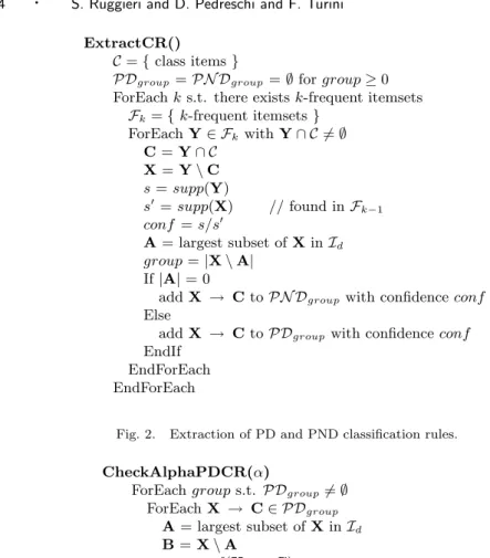
α-protective rules. This problem is solvable by directly checking the inequality of Def. 4.5 (resp., Def. 4.9), provided that the elements of the inequality are available. We define a checking algorithmCheckAlphaPDCR()in Fig. 3 that starts from the set of frequent itemsets, namely itemsets with a given minimum support. This is the output of any of the several frequent itemset extraction algorithms available at the FIMI repository [Goethals 2009]. The procedure ExtractCR() in Fig. 2 extracts PD and PND classification rules by a single scan over the frequent itemsets ordered by the itemset sizek. Fork-frequent itemsets that include a class item, a single classification rule is produced in output. The confidence of the rule can be computed by looking only at itemsets of lengthk−1. The rules in output are distin-guished between PD and PND rules, based on the presence of discriminatory items in their premises. Moreover, the rules are grouped on the basis of the sizegroupof the PND part of the premise. The output is a collection of PD rulesPDgroup and
a collection of PND rules PN Dgroup. TheCheckAlphaPDCR() procedure can
then calculate the extended lift of a classification ruleA,B → C∈ PDgroup from
its confidence and the confidence of the base ruleB → C∈ PN Dgroup.
The computational complexity in both time and space of the procedures presented in this paper is discussed in Appendix B.
ExtractCR()
C={class items}
PDgroup =PN Dgroup =∅forgroup≥0
ForEachks.t. there existsk-frequent itemsets
Fk={k-frequent itemsets} ForEachY∈ FkwithY∩ C 6=∅ C=Y∩ C X=Y\C s=supp(Y) s0 =supp(X) // found inF k−1 conf =s/s0 A= largest subset ofXinId group=|X\A| If|A|= 0
addX → CtoPN Dgroup with confidenceconf
Else
addX → CtoPDgroup with confidenceconf
EndIf EndForEach EndForEach
Fig. 2. Extraction of PD and PND classification rules.
CheckAlphaPDCR(α)
ForEachgroups.t. PDgroup6=∅
ForEachX → C∈ PDgroup
A= largest subset ofXinId
B=X\A
γ=conf(X → C)
δ=conf(B → C) // found inPN Dgroup
Ifelif t(γ, δ)≥α // resp.,glif t(γ, δ)≥α
outputA,B → C
EndIf EndForEach EndForEach
Fig. 3. Direct checking ofα-discrimination.
5.2 The German credit case study
In this section, we analyze the reference dataset in search of direct discrimination. We present the distributions of α-discriminatory PD rules at the variation of a few parameters that one can use to control the set of extracted rules: minimum support, minimum confidence, class item, and the setId of PD itemsets.
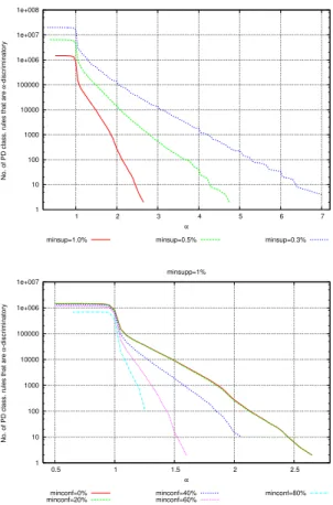
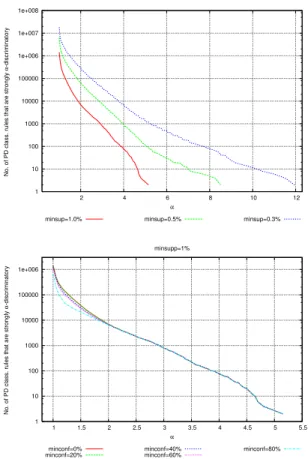
Discrimination w.r.t. support thresholds. The top plot in Fig. 4 (resp., Fig. 5) shows the distribution ofα-discriminatory PD rules (resp., strongα-discriminatory PD rules) for minimum supports of 1%, 0.5% and 0.3%. The figures highlight how lower support values increase the number of PD rules and the maximum α. Notice that, for a same minimum support, αreaches higher values in Fig. 5 than
1 10 100 1000 10000 100000 1e+006 1e+007 1e+008 1 2 3 4 5 6 7
No. of PD class. rules that are
α
-discriminatory
α
minsup=1.0% minsup=0.5% minsup=0.3%
1 10 100 1000 10000 100000 1e+006 1e+007 0.5 1 1.5 2 2.5
No. of PD class. rules that are
α -discriminatory α minsupp=1% minconf=0% minconf=20% minconf=40% minconf=60% minconf=80%
Fig. 4. The German credit dataset. Top: distributions ofα-discriminatory PD rules. Bottom: contribution of setting minimum confidence for base rules.
in Fig. 4, since strong α-discrimination of a rule implicitly takes into account the complementary class rule, which may have a support lower than the minimum (see e.g.,(a-bad)in Ex. 4.7). We report three sample PD rules with decreasing support and increasing extended lift.
a1. personal_status=female div/sep/mar, employment=1<=X<4 property_magnitude=real estate, job=skilled
==> class=bad
-- supp:(0.011) conf:(0.48) elift:(2.39)
a2. age=(52.6-inf), employment=1<=X<4, existing_credits=(1.6-2.2] ==> class=bad
-- supp:(0.005) conf:(1) elift:(3.60)
a3. age=(52.6-inf), employment=1<=X<4, savings_status=>=1000 ==> class=bad
1 10 100 1000 10000 100000 1e+006 1e+007 1e+008 2 4 6 8 10 12
No. of PD class. rules that are strongly
α
-discriminatory
α
minsup=1.0% minsup=0.5% minsup=0.3%
1 10 100 1000 10000 100000 1e+006 1 1.5 2 2.5 3 3.5 4 4.5 5 5.5
No. of PD class. rules that are strongly
α -discriminatory α minsupp=1% minconf=0% minconf=20% minconf=40% minconf=60% minconf=80%
Fig. 5. The German credit dataset. Top: distributions of strongly α-discriminatory PD rules. Bottom: contribution of setting minimum confidence for base rules.
Rule a1states that among the people employed since one to four years, having a real estate property and with skilled job, the status of being woman and not single leads to having assigned the bad credit class 2.39 times more than the average. The rule has confidence 48%, which means that the base rule has confidence 0.48/2.39 = 20%. Rule a2states that senior people employed since one to four years, having already two existing credits are assigned the bad credit class 3.6 times more than the average. Finally, rulea3reaches a lift of 9 when compared to the base rule:
employment=1<=X<4, savings_status=>=1000 ==> class=bad
-- supp:(0.002) conf:(0.11)
People with large savings are usually given good credit. However, only 2 cases out of 18 (i.e., 11%) are assignedclass=bad. Both of them are senior people!
Let us show next the elapsed time of the proceduresExtractCR()and Check-AlphaPDCR() on a 32-bit PC with Intel Core 2 Quad 2.4Ghz and 4Gb main memory. We also report the number (M=millions) of frequent itemsets in input to ExtractCR() and the number of PD and PND rules yielded in output. For
1 10 100 1000 10000 100000 1e+006 0.5 1 1.5 2 2.5 3
No. of PD class. rules that are
α -discriminatory α minsup=1.0% class=bad class=good 1 10 100 1000 10000 100000 1e+006 1 1.5 2 2.5 3 3.5 4 4.5 5 5.5
No. of PD class. rules that are strongly
α
-discriminatory
α minsup=1.0%
class=bad class=good
Fig. 6. The German credit dataset. Top: distribution ofα-discriminatory PD rules for each class item. Bottom: distribution of stronglyα-discriminatory PD rules.
frequent pattern extraction, any system from [Goethals 2009] can be adopted. All procedures reported in this paper are implemented in Java 6.
No. freq. ExtractCR() CheckAlphaPDCR() minsup itemsets No. PD No. PND Time Time
1% 6.6M 1.45M 1.27M 38s 13.5s
0.5% 26.8M 6.4M 5.3M 163s 55s
0.3% 79.0M 20.0M 15.9M 519s 165s
The elapsed times are consistent with the worst-case complexity analysis reported in Appendix B and show good scalability along with the minimum support threshold.
Discrimination w.r.t. confidence thresholds. Another widely adopted parameter for controlling rule generation is minimum confidence. The bottom plot in Fig. 4 shows how the confidence threshold of the base rule affects the distribution ofα -discriminatory PD rules. Higher confidence thresholds lead to fewer number of discriminatory rules and lower maximum extended lift values. This is consistent with the observation that the extended lift ranges over [0,1/mc], where mcis the minimum confidence threshold of base rules.
1 10 100 1000 10000 100000 1e+006 0.5 1 1.5 2 2.5 3
No. of PD class. rules that are
α
-discriminatory
α minsup=1.0%
class=bad class=good
Fig. 7. The German credit dataset. Distributions ofα-discriminatory PD classification rules for
I0
d={personal status=male single,age=(41.4-52.6]}.
On the contrary, acting on minimum confidence of the base rule does not result in an effective mechanism for unveiling additional stronglyα-discriminatory rules, as shown in Fig. 5 bottom plot.
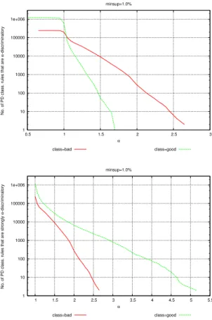
Discrimination w.r.t. class item. The contribution of the class item to the dis-tribution of discriminatory PD classification rules is shown in Figure 6, where the minimum support is fixed to 1%. The top plot highlights that rules with class item
class=badcontribute mostly to higher values of extended lift. This confirms that
the set of PD itemsetsIdfixed so far (see Ex. 4.2) characterizes groups of people that
are discriminated rather than favored. Also, notice that whenα <1, the number of PD rules with class itemclass=goodbecomes predominant. Since an extended lift lower than 1 means group under-representation, this leads to the dual conclusion that people characterized by Id are under-represented in benefit granting. Such a
dual behavior is explicitly taken into account by strongα-protection, which con-siders at the same time both under-representation and over-representation – or, in formal terms, extended lifts of bothA,B→class=goodandA,B→class=bad. As shown at the bottom plot in Figure 6, PD rulesA,B →class=good that al-low for inferring discrimination of the complementary ruleA,B→class=badare indeed the vast majority.
Discrimination w.r.t. the set of PD discriminatory itemsets. As highlighted by Figure 6 top plot, the set of discriminatory itemsets fixed so far leads mainly to discrimination againstassigning credit. There are, however, cases where discrimi-nationin favor of assigning credit is raised, as in the following:
personal_status=female div/sep/mar, property_magnitude=no known property employment=<1, other_parties=none ==> class=good
Women who are recently employed, with no known property, and no supporting party are assigned good credit score with a probability of 2.14 times the average one of people in the same conditions. This might reveal a good practice of enforcement of affirmative actions or other policies or laws in support of disadvantaged categories [Holzer and Neumark 2006].
Discrimination in favor of assigning credit can also reveal a malpractice of un-fair favoritism for certain categories. In order to illustrate this, however, we need to switch to a different set of discriminatory itemsets. Let us fix I0
d = {
perso-nal status=male single, age=(41.4-52.6]}, namely we are now interested in
discrimination in favor of male single and/or people in their 40’s. Figure 7 shows the distributions ofα-discriminatory PD rules for each class item. Contrasted to the Figure 6 top plot, classification rules with class item class=bad occur much less frequently and with lower values of extended lift, while rules with class item
class=good occur slightly more frequently and with slightly higher values of
ex-tended lift. This can be interpreted as favoring credit to people which are single man and/or in their 40’s.
6. INDIRECT DISCRIMINATION THROUGH BACKGROUND KNOWLEDGE 6.1 Motivating Example
Direct discrimination checking does not take into account PND classification rules, since they do not explicitly contain PD itemsets. Formally, a PND rule is 1-protective. In the case of indirect discrimination, as modelled in Fig. 1 right, one assumes the extreme case that PD itemsets are not available at all in the underlying dataset. Hence, only PND classification rules can be extracted. As discussed in Sect. 2, contexts of discriminatory decisions can still be unveiled in the form of PD classification rules by exploiting some additional background knowledge. Next we highlights an example over the German credit dataset.
Example 6.1. Consider again the German credit dataset, but assume now that PD itemsets have been removed from it. Also, consider the following context:
B= credit_history=critical/other existing credit
residence_since=(2.8-inf) savings_status=<100
checking_status=nochecking
The following PND classification rules can be extracted:
dbc. age=(-inf-30.2],B ==> class=bad -- conf:(0.167) bc. B ==> class=bad -- conf:(0.027)
Rule(dbc)states that young people in the contextBof people with critical credit
history, resident since 2.8 years at least, with savings at most for 100 units, and with no checkings, were assigned the bad credit scoring with a confidence of 16.7%. Rule(bc)is obtained from(dbc)by discarding the item age=(-inf-30.2]in the premise, and it has a confidence of 2.7%. As discussed in Sect. 2, without any further information, we cannot say whether rule(dbc) unveils any discrimination or not. Assume now to know (by some background knowledge) that in the context
B above, the set of persons satisfying age=(-inf-30.2] is somewhat related to the set of persons satisfying the PD itempersonal status=female div/sep/mar. If the two sets were exactly the same, we could replace age=(-inf-30.2]in rule
(dbc)with the PD item above. This would lead us to the PD classification rule:
abc. personal status=female div/sep/mar,B
==> class=bad
withglif t(0.167,0.027) = 6.19, which is considerably high.
In case the two sets of persons coincide only to some extent, we can still obtain some lower bound for theglif t() of(abc). In particular, assume that young people in the contextB, contrarily to the average case, are almost all non-single women:
dba. age=(-inf-30.2],B
==> personal_status=female div/sep/mar -- conf:(0.95)
Is this enough to conclude that non-single women in the context are discriminated? We cannot say that: for instance, if non-single women in the context are at 99% older than30.2 years, only the remaining 1% is involved in the decisions fired by
rule(dbc), hence women in the context cannot be discriminated by these decisions.
As a consequence, we need further information about the proportion of non-single women that are younger than30.2years. Assume to know that such a proportion is at least 70%, i.e. :
abd. personal status=female div/sep/mar,B
==> age=(-inf-30.2] -- conf:(0.7)
By means of the forthcoming Thm. 6.2, we can state that the rule (abc) is at least 3.19-discriminatory. This unveils that non-single women in the context were imposed a burden in credit denial of at least 3.19 times the average of people in the context. Since the German credit dataset contains the PD items, we can check how accurate is the lower bound by calculating the actualglif t() value for (abc): it turns out to be 3.37.
6.2 Inference Model
We formalize the intuitions of the example above in the next result, which derives a lower bound for (strong) α-discrimination of PD classification rules given infor-mation available in PND rules (γ, δ) and information available from background rules (β1,β2).
Theorem 6.2. Let D,B → C be a PND classification rule, and let: γ=conf(D,B → C) δ=conf(B → C)>0. Let Abe a PD itemset and letβ1, β2 such that:
conf(A,B → D)≥β1 conf(D,B → A)≥β2>0.
Called:
f(x) =β1
elb(x, y) = ½ f(x)/y iff(x)>0 0 otherwise glb(x, y) = f(x)/y iff(x)≥y f(1−x)/(1−y) iff(1−x)>1−y 1 otherwise we have: (i). 1−f(1−γ)≥conf(A,B → C)≥f(γ),
(ii). for α≥ 0, if elb(γ, δ) ≥ α, then the PD classification rule A,B → C is α-discriminatory,
(iii). forα ≥1, if glb(γ, δ) ≥α, then the PD classification rule A,B → C is
stronglyα-discriminatory. 2
Proof. See Appendix A.4.
Notice that the first two cases of the glb() function are mutually exclusive2, and that there is no division by zero3.
The ruleA,B → Destablishes how much the discriminatory features Aentail
Din the contextB, and, on the other side, the ruleD,B → Asays how much the non-discriminatory featuresDentailAin the same context. Together they provide the boundaries within which externally discovered discriminatory features can hide behind the non-discriminatory ones, given a contextB.
It is worth noting that β1 and β2 are lower bounds for the confidence values of A,B → D and D,B → A respectively. This amounts to stating that the correlation betweenAandDin contextBwithin the dataset must be known only with some approximation as background knowledge. Moreover, asβ1 and β2 tend to 1, the lower and upper bounds in (i)tend to γ. Also, f(γ) is monotonic w.r.t both β1 and β2, but an increase of β1 leads to a proportional improvement of the precision of lower and upper bounds, while an increase of β2 leads to a more than proportional improvement.
Example 6.3. Reconsider Ex. 6.1. We haveγ= 0.167, δ= 0.027, β1= 0.7, and
β2 = 0.95. The lower bound for the glif t() value of rule (abc) is computed as follows. Called:
f(x) = 0.7
0.95(0.95 +x−1),
we havef(0.167) = 0.086>0.027, andglb(0.833,0.973) =f(0.167)/0.027 = 3.19. Assume that the value ofconf(A,B → D) is known with an approximation of 5%, i.e.,β1= 0.665, whileβ2is unchanged. We havef(x) = 0.665/0.95(0.95+x−1), and sincef(0.167) = 0.082>0.027, we obtainglb(0.833,0.973) =f(0.167)/0.027 = 3.03, i.e., the inferred lower bound is proportionally (5%) lower. Assume now that
conf(D,B → A) is known with an approximation of 5%, i.e.,β2= 0.9 andβ1 is
2By conclusion(i), 1−f(1−γ)≥f(γ). Whenf(γ)≥δ, this implies 1−f(1−γ)≥f(γ)≥δand
thenf(1−γ)≤1−δ. Whenf(1−γ)>1−δ, this impliesδ >1−f(1−γ)≥f(γ).
3Iff(γ)≥δthen the divisor isδ >0. Consider now the casef(1−γ)>1−δand assume, by
unchanged. We havef(x) = 0.7/0.9(0.9 +x−1). Again f(0.167) = 0.052>0.027 impliesglb(0.833,0.973) =f(0.167)/0.027 = 1.93, which is more than proportion-ally lower than 3.19.
Recalling the redlining example from Sect. 2, an application of Thm. 6.2 allows us to conclude that black people (race=black) are discriminated in a context (city=NYC) because almost all people living in a certain neighborhood (neighborhood=10451) are blacks (this isβ2) and almost all black people live in that neighborhood (this is
β1). In general, this is not the case, since black people live in many different neigh-borhoods. Moreover, in the redlining example we had to provide, as background knowledge, only the approximationβ2. However, notice that the conclusion of the example is slightly different from the one above, stating that black people who live in a certain neighborhood (race=black, neighborhood=10451) are discriminated w.r.t. people in the context (city=NYC). Such an inference can be modelled as an instance of Thm. 6.2 that strictly requires a downward closed set of itemsets.
Example 6.4. Rules(a)and(c)from Sect. 2:
a. city=NYC c. neighborhood=10451, city=NYC
==> class=bad ==> class=bad
-- conf:(0.25) -- conf:(0.95)
are instances respectively of B → C and D,B → C in Thm. 6.2, with B =
city=NYC,D =neighborhood=10451 andC =class=bad. Hence,γ = 0.95 and
δ= 0.25. What should be a set of PD itemsets for reasoning about redlining? Cer-tainly,neighborhood=10451alone cannot be considered discriminatory. However, the pairA=race=black, neighborhood=10451might denote a possible discrimi-nation against black people in a specific neighborhood. In general, all conjunctions of items of minorities and neighborhoods is a source of potential discrimination. This set of itemsets is downward closed, albeit not in the form of 2J for a set of
items J. As background knowledge, we can now refer to census data, reporting distribution of population over the territory. So, we can easily gather statistics such as rule(d)from Sect. 2, which can be rewritten4 as:
d. neighborhood=10451, city=NYC ==> race=black, neighborhood=10451 -- conf:(0.8)
This is an instance of D,B → Ain Thm. 6.2. The other expected background rule isA,B → D, which readily has confidence 100%, i.e.,β1= 1, sinceAcontainsD. So, we have not to take it into account in this redlining example, which therefore represents a simpler inference problem than the one considered in Thm. 6.2. By the conclusion of the theorem, we obtain lower bounds for the confidence and the extended lift ofA,B → C, i.e., rule (e)from Sect. 2:
e. race=black, neighborhood=10451, city=NYC ==> class=bad
4Notice that, for an association ruleX → Y, we admitX∩Y6=∅. The assumptionX∩Y=∅
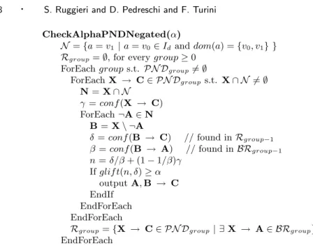
CheckAlphaPNDCR(α) Rg=∅, for everyg≥0 ForEachgs.t. PN Dg6=∅ Rg={X → C∈ PN Dg | ∃X → A∈ BRg} ForEachX → C∈ Rg γ=conf(X → C)
V =∅,generate= true // candidate contexts
ForEachX → A∈ BRg order byconf(X → A) descending
β2 =conf(X → A)
s =supp(X → A)
(i) Ifβ2>1−γorβ2> γ
Ifgenerate // lazy generation of candidate contexts
ForEachB⊆Xsuch thatB → C∈ Rg0 withg0=|B| ≤g
δ=conf(B → C) (iii) Ifβ2(1−αδ)≥1−γ orβ2(1−α(1−δ))≥γ V =V ∪ {(B, δ)} EndIf EndForEach generate= false EndIf ForEach (B, δ)∈ V (iii) Ifβ2(1−αδ)≥1−γ orβ2(1−α(1−δ))≥γ
β1 =s/supp(B → A) // found inBRg0 withg0=|B| ≤g
Ifglb(γ, δ)≥α
outputA,B → C
EndIf Else
V =V \ {(B, δ)} // no need to check it anymore EndIf EndForEach EndIf EndForEach EndForEach EndForEach
Fig. 8. Algorithm for checking indirect strongα-discrimination through background knowledge. HereBRg is{X → A∈ BR | |X|=g}.
Confidence of(e)is at least 1/0.8(0.8 + 0.95−1) = 0.9375, and then its extended lift (w.r.t. the contextcity=NYC) is at least 0.9375/0.25 = 3.75. Summarizing, the classification rule (e)is at least 3.75-discriminatory or, in simpler words, (c) is a redlining rule unveiling a “disproportionate burden” (of at least 3.75 times than the average of NYC people) over black-race people living in neighborhood 10451.
6.3 Checking the Inference Model
We measure the power of the inference model by defining theabsolute recallatαas the number ofα-discriminatory PD rules that are inferrable by Thm. 6.2 starting from the set of PND classification rulesPN Dand a set of background rules BR.
large set of background rules under the assumption that the dataset contains the discriminatory items, e.g., as in the German credit dataset. We define:
BR={X → A|XPND,APD, supp(X → A)≥ms},
as the set of association rulesX→Awith a given minimum support. While rules of the formA,B →Dseem not to be included in the background rule set, we observe thatconf(A,B → D) can be obtained assupp(D,B → A)/supp(B →A), where both rules in the ratio are of the required form. Notice that the set BRcontains the most precise background rules that an analyst could use, in the sense that the values forβ1 andβ2in Thm. 6.2 do coincide with the confidence values they limit. A straight implementation of the inference model consists of checking the condi-tions of Thm. 6.2 for each partitionD,Bof X, whereX → C is a rule inPN D. Since there are 2|X| of such partitions, we will be looking for some pruning
condi-tions that restrict the search space. Let us start considering necessary condicondi-tions forelb(γ, δ)≥α. Ifα= 0 the expression is always true, so we concentrate on the caseα >0. By definition ofelb(),elb(γ, δ)≥α >0 happens only if f(γ)>0 and
f(γ)/δ≥α, which can respectively be rewritten as:
(i)β2>1−γ (ii) β1(β2+γ−1)≥αδβ2.
Therefore,(i)is a necessary condition for elb(γ, δ)≥α. From(ii) andβ1 ≤1, we can concludeelb(γ, δ)≥αonly ifβ2+γ−1≥αδβ2, i.e.:
(iii)β2(1−αδ)≥1−γ.
Therefore, (iii) is a necessary condition for elb(γ, δ) ≥α as well. The selectivity of conditions (i,iii) lies in the fact that checking (i) involves no lookup at rules
B → C to compute δ=conf(B → C); and checking (iii)involves no lookup at the rule A, B → D to compute β1 = conf(A,B → D). Moreover, conditions
(i,iii)are monotonic w.r.tβ2, hence if we scan the association rulesX → Aordered by descending confidence, we can stop checking for a candidate context as soon as they are false. Finally, we observe that similar necessary conditions can be derived forglb(γ, δ)≥α.
The generate&test algorithm that incorporates the necessary conditions is shown in Fig. 8. As a space optimization, we prevent keeping the whole set of PND rules PN D, needed when searching forδ=conf(B → C), by keeping inRga PND rule
X → C only if there exists some background ruleX → A∈ BR. Otherwise, we could not even computeconf(B → A), needed for calculatingβ1. Computational complexity in both time and space of the CheckAlphaPNDCR() procedure is discussed in Appendix B.
6.4 The German credit case study
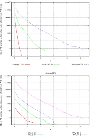
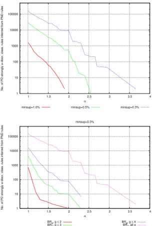
With reference to the presented test framework, Fig. 9 top plot shows the distri-bution of the absolute recall of the proposed inference model, at the variation of
αand minimum support. Even for high values ofα, the number of indirectly dis-criminatory rules is considerably high. As an example, for minimum support of 0.3%, 390 PD classification rules that are strongly 4-discriminatory can be inferred from PND rules. As one could expect, the absolute recall heavily depends on the size of the background knowledge. Fig. 9 bottom plot shows the distribution of the
1 10 100 1000 10000 100000 1e+006 1e+007 1 2 3 4 5 6 No. of PD strongly α
-discr. class. rules inferred from PND rules
α
minsup=1.0% minsup=0.5% minsup=0.3%
1 10 100 1000 10000 100000 1e+006 1e+007 1 2 3 4 5 6 No. of PD strongly α
-discr. class. rules inferred from PND rules
α minsup=0.3% BRg, g ≤ 3 BRg, g ≤ 4 BRg, g ≤ 5 BRg, all g
Fig. 9. The German credit dataset. Top: absolute recall of the inference model through back-ground knowledge at the variation of minimum support. Bottom: absolute recall at the variation of maximum length of background rules’ premise. HereBRgis{X → A∈ BR | |X|=g}.
absolute recall at the variation of the maximum length of background rules’ premise for a fixed minimum support of 0.3%. As an example, if we have background rules
X → Awith|X| ≤3, the best inference leads to two strongly 2.45-discriminatory rules. Highly discriminatory contexts can then be unveiled only starting from very fine-grained background knowledge.
We report below the execution times of theCheckAlphaPNDCR()procedure (on a 32-bit PC with Intel Core 2 Quad 2.4Ghz and 4Gb main memory) for rules in PN DandBRhaving minimum support of 1% and without/with the optimization checks discussed earlier. The set PN D consists of 1.27 millions of classification rules, and the setBR consists of 2.1 millions of association rules. Notice that the size ofBRis exceptionally large, since it is obtained starting from a dataset which already contains the PD itemsets. In real cases, only a limited number (in the order of thousands) of background rules are available from statistical sources, surveys or experts.
without checks with checks ratio
α= 2.0 434s 136s 31.3%
α= 1.8 434s 139s 32.0%
α= 1.6 434s 144s 33.2%
α= 1.4 434s 158s 36.4%
Whilst there is a gain in the execution time in using the optimizations, up to 68.7%, the order of magnitude is the same. This can be explained by observing that condition(i)allows for cutting generation&testing of candidates, but condition
(iii)allows for cutting only testing of candidates.
7. INDIRECT DISCRIMINATION THROUGH NEGATED ITEMS 7.1 Motivating Example
A limitation of the inference model based on background knowledge occurs when dealing with a binary attribute a such that a = v is PD and its negated item ¬(a=v) is PND. The most common case consists of the PD itemsex=female, and the PND itemsex=male. For D=sex=male, and A=sex=female, we have that the assumptionconf(D,B → A) = 0≥β2 >0 of Thm. 6.2 does not hold. As a conclusion, the inference model based on background knowledge cannot derive lower bounds for PND rules involving women starting from PD rules involving men. Such an inference is instead quite natural in practice. Notice that in the German credit dataset this case does not occur, since the attributesexis not binary.
Let us show next an example involving the attributeforeign worker, for which
foreign worker=no is PND whilst foreign worker=yes is PD. A rule including
foreign worker=no in its premise is considered PND. However, by reasoning as
done for binary classes in Sect. 4.3, such a rule can unveil α-discrimination of the PD rule obtained by replacingforeign worker=nowithforeign worker=yes.
Example 7.1. Consider again the German credit dataset, and assume that PD itemsets have been removed from it. Also, consider the following itemset:
B= personal_status=male single
employment=1<=X<4 purpose=new car housing=rent
The following PND classification rules can be extracted:
nbc. foreign worker=no,B ==> class=good -- conf:(1) bc. B ==> class=good -- conf:(0.9)
Rule(nbc)states that national workers in the contextBof people that are single
male, employed since one to four years, which intend to buy a new car, and have their house for rent, are assigned a good credit scoring with confidence 100%. Rule
bcstates that the average confidence of people in contextBis slightly less, namely 90%. It is quite intuitive that the increasing of confidence from 90% to 100%, yet being a small one, has to be attributed to the omission of foreign workers. Therefore, for the rule:
![Fig. 7. The German credit dataset. Distributions of α-discriminatory PD classification rules for I 0 d = { personal status=male single, age=(41.4-52.6] }.](https://thumb-us.123doks.com/thumbv2/123dok_us/527700.2562147/18.892.300.607.183.400/german-credit-dataset-distributions-discriminatory-classification-personal-status.webp)