Improving SVM Classification on Imbalanced
Datasets by Introducing a New Bias
Haydemar N´
u˜
nez
Central University of Venezuela, Venezuela
Luis Gonzalez-Abril
Universidad de Sevilla, Espa˜
na
Cecilio Angulo
Technical University of Catalonia, Spain
May 22, 2017
Abstract
Support Vector Machine (SVM) learning from imbalanced datasets, as well as most learning machines, can shows poor performance on the minority class because SVM were designed to induce a model based on the overall error. To improve their performance in this kind of problems, a low-cost post-processing strategy is proposed based on calculating a new bias to adjust the function learned by the SVM.
The proposed bias will consider the proportional size between classes in order to improve performance on the minority class. This solution avoids not only introducing and tuning new parameters, but also mod-ifying the standard optimization problem for SVM training.
Experimental results on 34 datasets, with different imbalance de-gree, show that the proposed method actually improves the classifi-cation on imbalanced datasets, by using standardized error measures based on sensitivity and g-means. Furthermore, its performance is comparable to well-known cost-sensitive and SMOTE schemes, with-out adding complexity or computational costs.
Keywords: Support Vector Machine, post-processing, bias, cost-sensitive strategy, SMOTE
1. Introduction
A major problem faced by classification learning algorithms is the imbalance between classes in datasets. It appears when there are many ex-amples of one or several classes, but very few in the remaining classes. Some domains where this situation arises are medical diagnosis, text classification, fraud detection in credit card usage, detection of communication network intrusion, among others. Since it usually represents the target of the classi-fication task, for such scenarios is very important to obtain models that ex-hibit a high prediction performance on the minority class. However, standard learning algorithms tend to produce hypothesis having a good performance only on the majority class, because they construct classification models based on error over the whole training set, independently of the representatives or balance between classes.
To solve this problem, some mechanisms exist to allow these algo-rithms showing good performance on minority class. To that effect, several strategies have been proposed, such as re-balancing the dataset with sam-pling techniques, construction of classifiers that take into account the cost of errors on different classes, combination (ensemble) of results from sev-eral classifiers trained with different data distributions (He and Garcia 2009; L´opez, Fern´andez, Garc´ıa, Palade, and Herrera 2013; Sun, Wong, and Kamel 2009).
In the case of SVM, its learning mechanism become an interesting option to deal with imbalanced datasets, because SVM build its classification model based only on a subset of training instances (Cristianini and Shawe-Taylor 2000; Vapnik 1999). However, like other machine learning techniques, SVM minimizes the error over all the dataset to generate these models, so they are biased towards the majority class when the imbalance is severe.
To enhance the performance of SVM for problems with imbalanced classes, several solutions have been proposed. Some of them are of gen-eral application, like sampling techniques to re-balancing datasets in a pre-processing stage; other, more specific, consider SVM’s particular features like those based on cost-sensitive learning (Batuwita and Palade 2013). Some re-search papers suggest using a post-processing stage in order to reduce the bias towards the majority class of the classifier learned by the SVM (He and Garcia 2009).
Following this last research line, a strategy for SVMs based on cal-culating a new bias or threshold is proposed. This new bias considers the classes’ proportion in the dataset and allows tuning the original function learned by the SVM to improve its performance on the minority class. Pro-posed solution neither introduces new parameters, nor modifies the original optimization problem for SVM training.
This paper is organized as follows: Section 2 briefly introduces the SVM learning mechanism and provides an overview of strategies to improve its performance on this kind of problems. In Section 3, the proposed post-processing procedure for determining the new bias is detailed. Section 4, presents the experiments performed to verify the applicability of the proposal, along with an analysis of results, and a comparison between performance of the new approach and a cost-sensitive scheme. Finally, conclusions and further research are presented.
2. SVM on Imbalanced Datasets
SVM is based on statistical learning theory and has been applied suc-cessfully in classification and regression problems in different domains (Cris-tianini and Shawe-Taylor 2000; Oneto, Ridella, and Anguita 2016; Vapnik 1999). The hypothesis spaces of these learning machines are hyperplanes (linear decision surfaces). Training looks for a decision function with the maximum margin of separation between classes. Thus, for a binary clas-sification task on a set of training data Z = {(x1, y1), . . . ,(xN, yN)}, with
xi ∈ X ⊆ <m,yi ∈ Y ={+1,−1}, and the decision functionf(x) = w·x−b,
the optimal hyperplane is determined as follows,
min w,b 1 2kwk 2 +C N X i=1 ξi s. t. yi(w·xi−b) +ξi ≥1, ξi ≥0, i= 1. . . N (1)
where w is the vector of the hyperplane which defines its orientation, and b is the bias which determines its position. Slack variables ξi measure the
error on the instances that violate the constraint yi(w·xi − b) ≥ 1. The
margin and minimizing the error, i.e. the higher the value of C, the SVM is more focused on minimizing errors. In a dual form, this optimization problem can be solved as,
max αi∈< N X i=1 αi− 1 2 N X i,k=1 αiyiαkykxi·xk s.t. 0≤αi ≤C, i= 1. . . N N X i=1 αiyi = 0, (2)
leading to the following decision function,
f(x) = sign N X i=1 αiyixi·x−b ! . (3)
To construct nonlinear decision boundaries, input vectors are pro-jected in an inner product space of higher dimension using a basis set of nonlinear functions. In this new space the optimal hyperplane is determined. Using the theory of kernels satisfying Mercer’s theorem, all operations can be performed directly in an input space using xi·xj =K(xi,xj). Then, the
decision function is formulated as,
f(x) = sign N X i=1 αiyiK(xi,xj)−b ! . (4)
Among all the training vectors, only a few have associated a weightαi
greater than zero in (3) or (4). These elements lie in the decision margin and are known as support vectors (SV). The unsigned valuef(x) is a measure of the distance of an example x to the hyperplane, while the sign determines the class label (positive or negative).
For moderately imbalanced datasets, empirical results show that, un-like other machine learning algorithms, SVM can produce a good hypothesis without any modification (Akbani, Kwek, and Japkowicz 2004; Imam, Ting, and Kamruzzaman 2006; Wu and Chang 2005). One explanation for such phenomenon is that SVM uses only a set of support vectors to construct clas-sification models, so negative instances that are far from the decision border will not be taken into account and SVM will not be affected by them, even
the numerous ones. However, SVM cannot overcome the problem of imbal-ance when data distribution is very imbalimbal-anced. In such cases, it has been observed that the hyperplane separation learned by the SVM is very close to the minority class, resulting in a low performance or no generalization at all for examples from this class, in comparison with those from the majority class (Batuwita and Palade 2013; He and Ghodsi 2010; Liu, An, and Huang 2006, Wu and Chang 2005).
2.1 Strategies for SVM with Imbalanced Datasets
Several strategies have been proposed to improve the performance of SVM on imbalanced datasets. Some of them are described and introduced in this section according to the moment that they can be applied during the learning process.
2.1.1 Pre-processing Strategies
They are based on re-sampling techniques to balance the dataset. One way is through the over-sampling of data from the minority class; hence, new instances are created in order to increase its proportion in the dataset. In contrast, under-sampling seeks to reduce the size of the majority class by removing a subset of these data. They are general-purpose procedures, not targeted at particular machine learning technique. One of the most commonly used is SMOTE, which employs thek-nearest neighbor technique for over-sampling the minority class (Chawla, Bowyer, Hall, and Kegelmeyer 2002; Vilari˜no, Spyridonos, Vitri`a, and Radeva 2005). Others strategies apply clustering algorithms for sub-sampling the majority class (Li, Yu, Bi and Huang 2014; Yu, Debenham, Jan, and Simoff 2006; Zhou, Ha, and Wang 2010).
There are also strategies for the SVM that seek increasing the minority class considering the margin area between the two classes (Castro, Carvalho, and Braga 2009). Other works are based on the use of SVM to obtain the positive support vectors, and over-sample from these data (Hern´ andez-Santiago, Cervantes, L´opez-Chau, and Garc´ıa-Lamont; Wang 2008). This feature has also been exploited to build under-sampling algorithms (Tang, Zhang, Chawla, and Krasse 2009; Wang 2014), where an SVM is used to build a new dataset composed only by the most informative negative support vectors and the positive data. Other solutions use sampling methods with
ensembles (Kang and Cho 2006; Liu et al. 2006; Waske, Benediktsson, and Sveinsso 2009; Yang, Zhang, Zhou, and Zomaya 2011; Sukhanov, Merentitis, Debes, Hahn and Zoubir 2015). Furthermore, there are proposals that seek over-sampling during training by using active learning (Ertekin 2013). 2.1.2 Training Strategies
These strategies include those proposals that modify the standard op-timization problem for SVM training in order to incorporate information related to the proportion of classes in the dataset. One approach of cost-sensitive learning is that incorporates into the learning problem information related with the penalties associated with wrong predictions for each class. In the case of SVM, the cost information about the two types of errors can be introduced into the formulation of the learning problem, using two regular-ization parameters, C+ and C−, associated with errors on the positive and
negative class, respectively (Ver-opoulos, Campbell, and Cristianini 1999; Cohen, Hilario, Sax, Hugonnet, and Geissbuhler 2006),
min w,b 1 2kwk 2+C+X i|yi=+1 ξi+C− X i|yi=−1 ξi s. t. yi(w·xi−b) +ξi ≥1, ξi ≥0, i= 1. . . N (5)
Some works have also added new restrictions on the slack variables ξi, in order to control the margin of separation between the two classes (He
and Ghodsi 2010; Yang, Wang, Yang, and Yu 2008). A different approach is presented in Batuwita and Palade (2010), where only one regularization parameterC is used, but information about the cost of errors is incorporated by allocating different weights to each variable ξi. Other proposed solutions
combine cost-sensitive learning with other techniques (Akbani et al. 2004; Muscat, Mahfouf, Zughrat, Yang, Thornton, Khondabiand, and Sortanos 2014; Wang and Japkowicz, 2010; Zi¸eba, Tomczak, Lubicz, and ´Swi¸atek 2014).
Other proposals are those that modify the kernel matrix according to the observed imbalance in the distribution of data, as KBA algorithm (Wu and Chang 2005). In Ram´ırez and Allende (2012) a method is proposed such that training two one-class SVM, one fitted to each class, and aggregating their decisions in a nested manner the boundary is improved. Finally, in
He, Wu, Silva, Zhao, and Qian (2015), a model-based approach integrat-ing cost-sensitive learnintegrat-ing with Gaussian Mixture Model for the imbalanced classification problem is proposed.
2.1.3 Post-processing Strategies
In general, these approaches are oriented either, towards modifying the weight vector w in the function of decision or determining a new bias, in order to adjust the decision boundary learned by the SVM to provide a good margin of separation for the positive class. For example, the z-SVM method is proposed in Imam et al. (2006), which determines the value of a new parameter z, solving an added optimization problem. This optimal parameter weights the contribution of support vectors of the minority class in the vector wof the decision function obtained after training.
In Li, Hu, and Hirasawa (2008), the bias of the decision function is modified by calculating an offset θ from the average of the unsigned values generated by f(x) for the support vectors. A similar strategy is used in Shanahan and Roma (2003), with the new offset being calculated by applying the Beta-Gamma algorithm.
Other studies suggest re-interpreting the outputs of the SVM. For example, a fuzzy decision function is applied in Li et al. (2008), whose parameters are estimated from the observed distribution in the dataset. In Wang and Zheng (2008), the decision process incorporates a post-processing module, whose construction is based on methods of information theory to define a new bias for classification.
3. A Novel Post-processing Strategy Based on the Bias Strategies proposed to improve the performance of SVM on imbal-anced datasets generally require tuning new parameters such as the sample rate or the number k of selected neighbors. Other methods can be computa-tionally expensive considering the construction of several classifiers (such as methods based on ensembles), or based on iterative algorithms, such as mod-ifying the kernel matrix (KBA) and some sampling techniques that require several over-training steps. In cost-sensitive approaches, the standard SVM optimization problem must be modified and costs of errors on the classes
must be known. Moreover, they can produce over-fitted models (Wang and Japkowicz 2010).
On the other hand, it has been empirically shown that the hyperplane learned by SVM in presence of imbalanced datasets have approximately the same orientation as the ideal hyperplane (He and Ghodsi 2010; Liu et al. 2006; Wu and Chang 2005). Reduced generalization on the minority class would be indeed associated with the bias b, as positive instances lie far from this ideal limit, i.e., the SVM learns a boundary that is too much close to this class. Other studies, such as those presented in Sun, Lim, and Liu (2009) at the domain of text classification, suggest increasing research on strategies determining new thresholds for the SVM’s decision function. Modifications should be based on the distribution of classes in the dataset, which also do not directly affect standard SVM training.
Following the latter research line, a novel post-processing strategy based on calculating of a new bias is proposed in this paper. The proportion among classes in the dataset will be considered, hence adjusting the function learned by the SVM in order to improve their performance on the minority class. The proposed solution does not involve tuning new parameters. Fur-thermore, it neither requires modifying the standard optimization problem for training the SVM, nor additional steps of re-training.
The proposal, based on the developments presented in Gonzalez-Abril, Angulo, Velasco, and Ortega (2008), modifies, after training, the separating margin of the hyperplane towards the majority class in order to achieve better generalization performance on data from the minority class. The new bias is calculated as follows (N´u˜nez, Gonzalez-Abril, and Angulo 2011).
LetZ ={(x1, y1), . . . ,(xN, yN)}be a training set, withxi ∈ X ⊆ <m,
yi ∈ Y = {+1,−1}. Also, let Z1 and Z2 be the datasets belonging to the positive class (+) and the negative one (-), respectively. The standard formulation of the bias, for the linearly separable case indicates that bias could be obtained as,
bs=
α+β
2 (6)
(bs = bstandard) where α is the maximum value of the hyperplane without
bias applied to the set of negative instances Z2, andβ is the minimum value of the hyperplane without bias applied to the entries in the minority set Z1,
that is, α= max xk∈Z2 N X i=1 αiK(xi,xk), and β = min xk∈Z1 N X i=1 αiK(xi,xk). (7)
Let us indicate that if the biasbis chosen asb=β, then all instance of the positive class are correctly labeled. Furthermore, β is the smallest value that ensures a 100% correct classification of the training vectors (Gonzalez-Abril, N´u˜nez, Angulo, and Velasco 2014).
Definition for bs in (6) has been extended for taking into account the
proportion of classes in the dataset. Hence, forN1 andN2 being the number of patterns in classes (+) and (-) respectively, a new proportional bias bp is
defined,
bp =
N1α+N2β N1 +N2
. (8)
Hence, for imbalanced problems, N1 N2, this new bias will move the decision limit towards the negative class, thus increasing the margin of separation for the positive class. Moreover, as the maximum and minimum values for the hyperplane without bias are reached on support vectors, it can be considered only these points for calculation of α and β,
α= max xk∈SV2 N X i=1 αiK(xi,xk), and β = min xk∈SV1 N X i=1 αiK(xi,xk) (9)
where SV1 and SV2 are the set of support vector in classes (+) and (-), respectively. The new decision function would simply be expressed as follows,
f(x) = sign N X i=1 αiyiK(xi,xj)−b ! . (10)
Furthermore, as the SVM decision function is generated only from the support vectors (the most informative instances for the classification task), an additional modification to this proposal exists: to consider the number of support vectors for the positive and negative classes, Nsv1 and Nsv2, respectively, rather than values N1 and N2.
Hence, a second bias bp1 is also proposed, bp1 =
Nsv1α+Nsv2β Nsv1+Nsv2
Let us see the relationship among these biases for N1 N2. In this case, the optimization problem usually provides a number of support vectors such that Nsv1 < Nsv2 and, defining R = N2/N1 and r = Nsv2/Nsv1, then 1≤r≤R (this fact can be checked in Section 4). Hence, it results,
|β−bp| = 1 1 +R |β−α|, |β−bp1| = 1 1 +r |β−α|, |β−bs| = 1 2|β−α|, (12) and 0≤ |β−bp| ≤ |β−bp1| ≤ |β−bs| (13)
that is, bs is farther from β than bp1, that in its turn, is farther away from β than bp. Thus, it can be checked that the decision function is moving
away from the zone of the positive samples, increasing, as it will be later demonstrated, the accuracy on this class. Therefore, these new biases move the hyperplane learned by SVM to obtain a better classification performance for the positive class, considering the proportions of the classes: the greater the imbalance, the greater margin of separation for the minority class.
4. Experimentation and Results Analysis
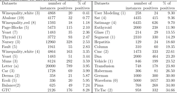
Performance of post-processing strategy proposed was tested on 34 datasets from the UCI repository (Frank and Asuncion 2010). Characteristics of the datasets are shown in Table 1. Label (+) was assigned to the class shown in brackets, and label (-) to the remaining data. The performance of the classifiers obtained by using the new biases was measured using sensitivity and geometric mean (g-means) (He and Garcia, 2009). Sensitivity measures positive accuracy, indicating how many examples of the minority classes are correctly classified; g-means evaluates the performance in terms of sensitivity and specificity (negative accuracy) as follows,
Table 1: UCI datasets used in the experimentation. These datasets are ordered from extreme to moderate imbalance.
Datasets number of % of Datasets number of % of instances positives positives instances positives positives Winequality white (3) 4868 20 0.41 User Modeling (1) 258 24 9.30 Abalone (19) 4177 32 0.77 Sat (4) 4435 415 9.36 Winequality red (8) 1593 18 1.18 Satimage (4) 6435 626 9.70 Page-Blocks (5) 5473 115 2.10 Euthyroid 2000 238 11.90 Yeast (7) 1483 35 2.36 Glass (7) 214 29 13.55 Thyroid (1) 3772 93 2.47 Segment (1) 2310 330 14.29 Nursey (3) 12960 328 2.53 Hepatitis 129 24 18.60 Fault (5) 1941 55 2.83 Column 310 60 19.35 Winequality white (4) 4864 163 3.35 Cmc (2) 1473 333 22.61 Yeast (5) 1483 51 3.44 Dna 2000 464 23.20 Muns (3) 8124 292 3.59 Vehicle (1) 846 199 23.52 Letter (a) 20000 789 3.95 Transfusion 748 178 23.80 Car (3) 1728 69 3.99 Haberman 306 81 26.50 Derma (2) 358 21 5.87 German 1000 300 30.00 Ecoli (5) 336 20 5.95 Waveform (0) 5000 1657 33.00 Balance(2) 625 49 7.24 Pima 768 268 34.00 GTC 2126 176 8.28 TicTac (2) 958 332 34.66
Sensitivity allows us to show how well the positive class is classified and g-means shows the balance between the accuracy of positive and neg-ative classes. Also, accuracy was included, as being the standard metric. For SVM training, the usual RBF kernel was used, as well as the Matlab’s Bioinformatics Toolbox for processing. The values of σ (RBF width) and C (regularization term) were obtained by exploring a two-dimensional grid: σ = {20,21, . . . ,26}, C = {20,21, . . . ,210} and the best values for accuracy for each classifier (SVM, cost-sensitive SVM and SMOTE SVM) were used.
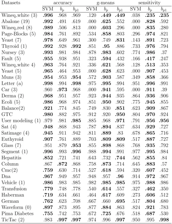
Average values for accuracy, g-means and sensitivity are shown in Table 2, for each dataset, using ten-fold cross-validation like empirical exper-imentation and repeating this procedure 10 times in order to ensure a good statistical behavior. From these results some statements can be established: • Working with imbalanced datasets, evaluation metrics like g-means and sensitivity measure the classifiers performance independently of the data distribution, so their election is correct for this kind of problems. For example, SVM has an accuracy value of 0.99 over Abalone dataset. However, it completely fails classifying the positive class, which is re-flected in the value of g-means.
Table 2: Average values for accuracy, g-means and sensitivity for each dataset, using ten-fold cross-validation (100 replications).
Datasets accuracy g-means sensitivity
SVM bp bp1 SVM bp bp1 SVM bp bp1 Wineq white (3) .996 .968 .969 .120 .449 .449 .038 .235 .235 Abalone (19) .992 .491 .619 .000 .625 .552 .000 .828 .592 Wineq red (8) .989 .506 .813 .000 .603 .296 .000 .835 .280 Page-Blocks (5) .984 .761 .892 .534 .858 .803 .296 .974 .821 Yeast (7) .978 .649 .961 .300 .749 .831 .143 .891 .723 Thyroid (1) .992 .928 .992 .851 .95 .886 .733 .976 .794 Nursey (3) .993 .981 .984 .878 .983 .602 .774 .986 .37 Fault (5) .955 .938 .951 .323 .594 .432 .166 .417 .247 Wineq white 4) .963 .764 .921 .336 .621 .568 .128 .513 .353 Yeast (5) .965 .464 .953 .000 .628 .623 .000 .907 .453 Muns (3) .954 .953 .954 .572 .903 .587 .349 .858 .366 Letter (a) .998 .994 .998 .975 .995 .994 .951 .996 .991 Car (3) .960 .973 .968 .000 .941 .595 .000 .911 .39 Derma (2) .968 .951 .957 .923 .944 .935 .864 .936 .906 Ecoli (5) .986 .968 .974 .851 .950 .902 .775 .945 .855 Balance(2) .921 .774 .845 .749 .830 .851 .623 .909 .867 GTC .980 .882 .975 .912 .920 .950 .804 .970 .924 User modeling (1) .979 .981 .985 .885 .968 .971 .791 .956 .956 Sat (4) .948 .868 .943 .787 .894 .837 .634 .929 .727 Satimage (4) .945 .911 .942 .811 .889 .83 .678 .865 .716 Euthyroid .907 .761 .889 .703 .809 .809 .517 .887 .727 Glass (7) .951 .879 .953 .855 .898 .868 .768 .935 .792 Segment (1) .996 .993 .996 .988 .994 .991 .977 .995 .984 Hepatitis .852 .721 .741 .643 .732 .744 .562 .855 .84 Column .867 .872 .868 .758 .873 .714 .645 .883 .57 Cmc(2) .759 .630 .714 .527 .618 .594 .320 .607 .452 Dna .967 .949 .957 .948 .957 .96 .914 .972 .967 Vehicle (1) .986 .983 .985 .982 .985 .985 .975 .988 .986 Transfusion .779 .748 .778 .540 .614 .557 .327 .462 .350 Haberman .719 .634 .661 .464 .617 .609 .273 .606 .512 German .762 .623 .708 .667 .660 .695 .517 .804 .680 Waveform (0) .897 .873 .895 .877 .884 .863 .824 .921 .783 Pima Diabetes .755 .742 .753 .672 .725 .676 .518 .687 .530 TicTac (2) .983 .997 .997 .974 .996 .997 .950 .995 .998
• For some datasets, despite the imbalance, the original SVM can get a reasonable model (e.g. Ecoli); but in other cases, it fails (Abalone, Winequality, Yeast).
• The new biases improve the performance of the standard SVM in all datasets with respect to g-means and sensitivity metrics. Furthermore, the performance on the sensitivity metric when using the bp bias is
better than employing bp1, in all datasets except for Tic-Tac dataset. This fact is due to that the Tic-Tac dataset is the unique of the 34 datasets such that r ≤R is not true.
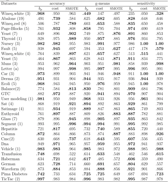
To compare the performance of this post-processing strategy with other reported in the literature, both, SMOTE and a cost-sensitive scheme were used to train a SVM on the listed UCI datasets. Comparison was only made with the bp bias. The Matlab Bioinformatic’s toolbox provides a
cost-sensitive scheme where the values for C+ and C− in (5) are calculated from
C as: C+ =C N 2N1 , and C− =C N 2N2 . (15)
It is worth noting that from the above, C = C+N1+C−N2
N1+N2 , that is, a similar
formula to the bias bp by changing C+ and C− for α and β, respectively.
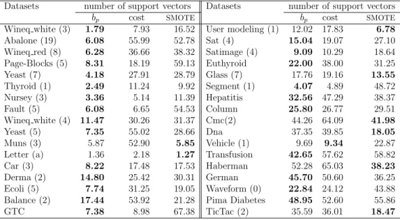
Results obtained using the same evaluation metrics, as well as the same ten-fold cross-validation structure, are shown in Table 3. Moreover, a comparison about the proportion of support vectors of the learned decision function in relation with the number of training data is offered for all the schemes in Table 4. This ratio is a measure of the complexity of the SVM classifier. Therefore, it can be concluded than both, SMOTE and cost sen-sitive approaches provide a decision function more complex and hence, as aforementioned, they can produce over-fitted models.
In order to measure the similarity of results between schemes, the Friedman test was applied (Demser 2006). This is a non-parametric test used to detect significant differences in multiple classifiers. The obtained p-values for accuracy, g-means and sensibility are 0.1076, 0.0150 and 0.0083, respectively. From these results, if a confidence level is fixed to 5%, it can be concluded the following:
• For the accuracy measure, as long as the p-value in the Friedman test is 0.1076, it can be concluded that there is no significant evidence of equivalence for the three methods.
Table 3: Comparison of the novel method vs the cost-sensitivity and SMOTE approaches. Average values for accuracy, g-means and sensitivity for each dataset, using ten-fold cross-validation.
Datasets accuracy g-means sensitivity
bp cost SMOTE bp cost SMOTE bp cost SMOTE Wineq white (3) .968 .950 .963 .449 .147 .497 .235 .050 .328 Abalone (19) .491 .739 .584 .625 .682 .605 .828 .648 .646 Wineq red (8) .506 .787 .789 .603 .653 .588 .835 .650 .458 Page-Blocks (5) .761 .932 .808 .858 .795 .704 .974 .690 .619 Yeast (7) .649 .896 .902 .749 .875 .876 .891 .860 .853 Thyroid (1) .928 .975 .989 .950 .957 .885 .976 .934 .795 Nursey (3) .982 .982 .955 .983 .991 .977 .986 1.00 1.00 Fault (5) .938 .945 .697 .594 .353 .627 .417 .178 .579 Wineq white (4) .764 .839 .897 .621 .657 .627 .513 .515 .441 Yeast (5) .464 .867 .863 .628 .843 .871 .911 .834 .775 Muns (3) .953 .962 .964 .903 .951 .981 .858 .939 .998 Letter (a) .994 .997 .998 .995 .997 .995 .996 .995 .991 Car (3) .973 .899 .903 .941 .946 .948 .911 1.00 1.00 Derma (2) .951 .931 .904 .944 .935 .917 .936 .944 .939 Ecoli (5) .968 .943 .945 .950 .976 .959 .945 1.00 .978 Balance(2) .774 .584 .813 .830 .781 .801 .909 .684 .796 GTC .882 .972 .887 .920 .941 .894 .970 .907 .904 User modeling (1) .981 .950 .949 .968 .933 .926 .956 .961 .904 Sat (4) .868 .919 .921 .894 .892 .863 .929 .861 .799 Satimage (4) .911 .934 .919 .889 .847 .863 .865 .749 .803 Euthyroid .761 .897 .887 .809 .826 .883 .887 .782 .881 Glass (7) .879 .896 .945 .898 .905 .897 .935 .863 .842 Segment (1) .993 .995 .996 .994 .994 .991 .995 .992 .985 Hepatitis .721 .817 .695 .732 .740 .589 .855 .720 .440 Column .872 .864 .866 .873 .874 .887 .883 .898 .926 Cmc(2) .630 .668 .737 .618 .643 .595 .607 .556 .435 Dna .949 .971 .965 .957 .959 .955 .972 .941 .937 Vehicle (1) .983 .983 .964 .985 .983 .972 .988 .985 .988 Transfusion .748 .698 .522 .614 .633 .548 .462 .546 .615 Haberman .634 .721 .642 .617 .485 .572 .606 .359 .490 German .623 .728 .714 .660 .691 .657 .804 .629 .557 Waveform (0) .873 .884 .853 .884 .888 .856 .921 .901 .866 Pima Diabetes .742 .733 .634 .725 .725 .649 .687 .694 .723 TicTac (2) .997 .983 .984 .996 .983 .982 .995 .987 .978
• With respect to the g-mean metric, as the p-value is 0.0150, the Fried-man test detected significant differences. Furthermore, the test indi-cates that there is not significant difference between post-processing strategy and cost-sensitive SVM methods. Nevertheless, there is
evi-Table 4: Proportion of support vectors in relation with the number of training data.
Datasets number of support vectors Datasets number of support vectors
bp cost SMOTE bp cost SMOTE
Wineq white (3) 1.79 7.93 16.52 User modeling (1) 12.02 17.83 6.78
Abalone (19) 6.08 55.99 52.78 Sat (4) 15.04 19.07 27.10 Wineq red (8) 6.28 36.66 38.32 Satimage (4) 9.09 10.29 18.64 Page-Blocks (5) 8.31 18.19 59.13 Euthyroid 22.00 38.00 31.25 Yeast (7) 4.18 27.91 28.79 Glass (7) 17.76 19.16 13.55 Thyroid (1) 2.49 11.24 9.92 Segment (1) 4.07 4.89 48.72 Nursey (3) 3.36 5.14 11.39 Hepatitis 32.56 47.29 38.37 Fault (5) 6.08 6.65 54.53 Column 25.80 26.77 29.51 Wineq white (4) 11.47 30.26 31.37 Cmc(2) 44.26 64.09 41.98 Yeast (5) 7.35 55.02 28.66 Dna 37.35 39.85 18.05 Muns (3) 5.87 52.90 5.85 Vehicle (1) 9.69 9.34 22.87 Letter (a) 1.36 2.18 1.27 Transfusion 42.65 57.62 58.82 Car (3) 8.22 17.48 17.53 Haberman 52.28 65.03 38.23
Derma (2) 14.80 25.42 30.31 German 45.70 50.60 36.25 Ecoli (5) 7.74 31.25 19.05 Waveform (0) 22.84 24.12 43.88 Balance (2) 17.44 53.92 21.28 Pima Diabetes 48.95 52.60 55.86 GTC 7.38 8.98 67.38 TicTac (2) 35.59 36.01 18.47
dence that these classifiers and SMOTE are significantly different. • With respect to the sensitivity measure, the p-value is 0.0083, that is,
the Friedman test detected significant differences. Furthermore, the test indicates us that there is significant difference among the post-processing strategy and the other two methods. Therefore, it can be concluded that the post-processing strategy is the best strategy in order to maximize the sensitivity metrics.
5. Conclusions an Future Work
From the experimental results on datasets with different degrees of imbalance, we can conclude that SVM performance is significantly improved using a new bias that considers the proportion of classes. An important benefit of the proposed approach is that the standard optimization problem associated to the SVM is not modified.
Neither new parameters must be tuned, so the computational cost is practically insignificant. By comparing this strategy with the cost-sensitive
and SMOTE approaches, the bias modification approach achieves superior performance in terms of sensitivity, and it does with a classification function far less complex in terms of number of support vectors.
As future work, a theoretical framework for studying the movements of the bias in the workspace according to their definition is being developed.
References
AKBANI, R., KWEK, S., and JAPKOWICZ, N. (2004), “Applying Support Vector Machines to Imbalanced Datasets”, in Proceedings of 15th European Conference on Machine Learning ECML’2004, pp. 39–50.
BATUWITA, R. and PALADE, V. (2010), “FSVM-CIL: Fuzzy Support Vector Machines for Class Imbalance Learning”, IEEE Transactions on Fuzzy Sys-tems, 18, 558–571.
BATUWITA, R. and PALADE, V. (2013), “Class Imbalance Learning Methods for Support Vector Machines”, in Imbalanced Learning: Foundations, Al-gorithms, and Applications, pp. 83-99, Berlin, Germany: John Wiley & Sons.
CASTRO, C. L., CARVALHO, M. A., and BRAGA, A. P. (2009), “An Improved Algorithm for SVMs Classification of Imbalanced Data Sets”, in Proceed-ings of 11th International Conference on Enginnering Applications of Neural Networks EANN 2009, pp. 108–118.
CHAWLA, N. V., BOWYER, K. W., HALL, L. O., and KEGELMEYER, W. P. (2002), “SMOTE: Synthetic minority over-sampling technique”, Journal of Artificial Intelligence Research, 16, 321–357.
COHEN, G., HILARIO, M., SAX, H., HUGONNET, S., and GEISSBUHLER, A. (2006), “Learning from imbalanced data in surveillance of nosocomial infection”, Artificial Intelligence in Medicine, 37, 7–18.
CRISTIANINI, N. and SHAWE-TAYLOR, J. (2000),An Introduction to Support Vector Machines and Other Kernel-based Learning Methods, New York, NY: Cambridge University Press, 1st Edition.
DEMSER, J. (2006), “Statistical comparisons of classifiers over multiple data sets, Journal of Machine Leaning Research, 7, 1–30.
ERTEKIN, S. (2013), “Adaptive Oversampling for Imbalanced Data Classifi-cation”, in Information Sciences and Systems, Lecture Notes in Electrical Engineering, 264, 261–269.
FRANK, A. and ASUNCION, A. (2010), UCI Machine Learning Repository, Uni-versity of California, School of Information and Computer Science. Irvine. archive.ics.uci.edu/ml
GONZALEZ-ABRIL, L., N ´U ˜NEZ, H., ANGULO, C., VELASCO, F. (2014), “GSVM: An SVM for Handling Imbalanced Accuracy Between Classes in Bi-classification Problems”,Applied Soft Computing, 17, 23-31.
GONZALEZ-ABRIL, L., ANGULO, C., VELASCO, F., and ORTEGA, J. A. (2008), “A Note on the Bias in SVMs for Multiclassification”,IEEE Trans-actions on Neural Networks, 19(4), 723–725.
HE, H. and GARCIA, E. A. (2009), “Learning from imbalanced data”, IEEE Transactions on Knowledge and Data Engineering, 21(9), 1263–1284. HE, H. and GHODSI, A. (2010), “Rare Class Classification by Support Vector
Machine”, in Proceedings 20th International Conference on Pattern Recog-nition, ICPR’10, pp. 548–551.
HERN ´ANDEZ-SANTIAGO, J., CERVANTES, J., CHAU, A. L., and GARC´IA-LAMONT, F. (2012), “Enhancing the Performance of SVM on Skewed Data Sets by Exciting Support Vectors”, in Proceedings of 13th Ibero-American Conference on Artificial Intelligence IBERAMIA 2012, pp. 101–110. IMAM, T., TING, K. M., and KAMRUZZAMAN, J. (2006), “z-SVM: An SVM
for Improved Classification of Imbalanced Data”, inProceedings of 19th Aus-tralian Conference on Artificial Intelligence AUS-AI 2006, pp. 264–273. KANG, P. and CHO, S. (2006), “EUS SVMs: Ensemble of Under-Sampled SVMs
for Data Imbalance Problems, Lecture Notes in Computer Science, 4232, 837–846.
LI, B., HU, J., and HIRASAWA, K. (2008), “An Improved Support Vector Ma-chine with Soft Decision-making Boundary”, inProceedings of 26th IASTED International Conference on Artificial Intelligence and Applications AIA’08, pp. 40–45.
LI, P., YU, X., BI, T. T., and HUANG, J. L. (2014), “Imbalanced Data SVM Classification Method Based on Cluster Boundary Sampling and DT-KNN Pruning”,International Journal of Signal Processing, Image Processing and Pattern Recognition, 7(2), 61-68.
LIU, Y., AN, A., and HUANG, X. (2006), “Boosting Prediction Accuracy on Imbalanced Datasets with SVM Ensembles”, inProceedings of 10th Pacific-Asia Conference on Knowledge Discovery and Data Mining PAKDD 2006, pp. 107–118.
L ´OPEZ, V., FERN ´ANDEZ, A., GARC´IA, S., PALADE, V., and HERRERA, F. (2013), “An Insight Into Classification with Imbalanced Data: Empir-ical Results and Current Trends on Using Data Intrinsic Characteristics”,
Information Sciences, 250, 113–141.
MUSCAT, R., MAHFOUF, M., ZUGHRAT, A., YANG, Y. Y., THORNTON, S., KHONDABI, A. V., and SORTANOS, S. (2014), “Hierarchical Fuzzy Support Vector Machine (SVM) for Rail Data Classification”, inProceedings of 19th IFAC World Congress, pp. 10652–10657.
NGUYEN, H. M., COOPER, E. W., and KAMEI, K. (2011), “Borderline Over-sampling for Imbalanced Data Classification”,International Journal of Knowl-edge Engineering and Soft Data Paradigms, 3, 4–21.
N ´U ˜NEZ, H., GONZALEZ-ABRIL, L., and ANGULO, C. (2011), “A Post-processing Strategy for SVM Learning from Unbalanced Data”, in Proceedings 19th European Symposium on Artificial Neural Networks ESANN’2011, pp. 195– 200.
ONETO, L., RIDELLA, S., and ANGUITA, D. (2016). “Tikhonov, Ivanov and Morozov Regularizationfor Support Vector Machine Learning,Machine Learning, 3, 103136.
RAM´IREZ, F. and ALLENDE, H. (2012), “Dual Support Vector Domain De-scription for Imbalanced Classification”, in Artificial Neural Networks and Machine Learning ICANN 2012,Lecture Notes in Computer Science, 7552, 710–717.
SHANAHAN, J. G. and ROMA, N. (2003), “Improving SVM Text Classification Performance Through Threshold Adjustment”, Lecture Notes in Computer Science, 2837, pp. 361–372.
SUKHANOV, S., MERENTITIS, A., DEBES, C., HAHN, J., ZOUBIR, A. (2015), “Bootstrap-based SVM Aggregation for Class Imbalance Problems”, in Pro-ceedings of 23rd European Signal Processing Conference EUSIPCO 2015, pp 155–169.
SUN, A., LIM, E.-P., and LIU, Y. (2009), “On Strategies for Imbalanced Text Classification Using SVM: A Comparative Study”, Decision Support Sys-tems, 48, 191–201.
SUN, Y., WONG, A. C., and KAMEL, M. S. (2009), “Classification of Imbal-anced Data: A Review”, International Journal of Pattern Recognition and Artificial Intelligence, 23, 687–719.
modeling for highly imbalanced classification”, IEEE Transactions on Sys-tems, Man and Cybernetics–Part B, 39, 281–288.
VAPNIK, V. N. (1999), The Nature of Statistical Learning Theory (Information Science and Statistics), New York, NY: Springer.
VEROPOULOS, K., CAMPBELL, C., and CRISTIANINI, N. (1999), “Control-ling the Sensitivity of Support Vector Machines”, in Proceedings of 16th International Joint Conference on Artificial Intelligence IJCAI 1999, pp. 55–60.
VILARI ˜NO, F., SPYRIDONOS, P., VITRI `A, J., and RADEVA, P. (2005), “Ex-periments with SVM and Stratified Sampling with an Imbalanced Problem: Detection of Intestinal Contractions”, in Proceedings of 3rd International Conference on Advanced Pattern Recognition ICAPR 2005, vol. 2, pp. 783– 791.
WANG, B. X. and JAPKOWICZ, N. (2010), “Boosting Support Vector Machines for Imbalanced Data Sets,Knowledge Information Systems, 25, 1–20. WANG, H. and ZHENG, H. (2008), “An Improved Support Vector Machine for
the Classification of Imbalanced Biological Datasets”, in Proceedings of 4th International Conference on Intelligent Computation ICIC 2008, pp. 63–70. WANG, H.-Y. (2008), “Combination Approach of SMOTE and Biased-SVM for Imbalanced Datasets”, in Proceedings of International Joint Conference on Neural Networks IJCNN 2008, pp. 228–231.
WANG, Q. (2014), “A Hybrid Sampling SVM Approach to Imbalanced Data Classification”, Abstract and Applied Analysis, Article ID 972786.
WASKE, B., BENEDIKTSSON, J. A., and SVEINSSON, J. R. (2009), “Classi-fying Remote Sensing Data with Support Vector Machines and Imbalanced Training Data”, in Proceedings of 8th International Workshop on Multiple Classifier Systems MCS09, pp. 375–384.
WU, G. and CHANG, E. Y. (2005), “KBA: Kernel Boundary Alignment Con-sidering Imbalanced Data Distribution”, IEEE Transactions on Knowledge and Data Engineering, 17, 786–795.
YANG, C.-Y., WANG, J., YANG, J.-S., and YU, G.-D. (2008), “Imbalanced SVM Learning with Margin Compensation”, in Proceedings of 5th International Symposium on Neural Networks: Advances in Neural Networks ISNN’08, pp. 636–644.
YANG, P., ZHANG, Z., ZHOU, B. B., and ZOMAYA, A. Y. (2011), “Sample Subset Optimization for Classifying Imbalanced Biological Data”, in
Pro-ceedings of 15th Pacific-Asia Conference on Advanced Knowledge Discovery and Data Mining PAKDD 2011, vol. 2, pp. 333–344.
YU, T., DEBENHAM, J., JAN, T., and SIMOFF, S. (2006), “Combine Vector Quantization and Support Vector Machine for Imbalanced Datasets”, in
Artificial Intelligence in Theory and Practice. IFIP 19th World Computer Congress, vol. 217, chapter 9, pp. 81–88.
ZHOU, B., HA, M., and WANG, C. (2010), “An Improved Algorithm of Un-balanced Data SVM”, Advances in Intelligent and Soft Computing, Fuzzy Information and Engineering, 78, pp. 549-555.
ZIE¸ BA, M., TOMCZAK, J. M., LUBICZ, M., and ´SWIA¸ TEK, J. (2014), “Boosted SVM for Extracting Rules from Imbalanced Data in Application to Predic-tion of the Post-operative Life Expectancy in the Lung Cancer Patients”,