Change-points Estimation in Statistical Inference and Machine Learning Problems

(1)

Worcester Polytechnic Institute

Digital WPI

Doctoral Dissertations (All Dissertations, All Years) Electronic Theses and Dissertations

2017-08-14

Change-points Estimation in Statistical Inference

and Machine Learning Problems

Bingwen Zhang

Worcester Polytechnic Institute

Follow this and additional works at:https://digitalcommons.wpi.edu/etd-dissertations

This dissertation is brought to you for free and open access byDigital WPI. It has been accepted for inclusion in Doctoral Dissertations (All Dissertations, All Years) by an authorized administrator of Digital WPI. For more information, please [email protected]. Repository Citation

Zhang, B. (2017).Change-points Estimation in Statistical Inference and Machine Learning Problems. Retrieved from https://digitalcommons.wpi.edu/etd-dissertations/344

(2)

Change-points Estimation in Statistical Inference and Machine

Learning Problems

by Bingwen Zhang

A Thesis

Submitted to the Faculty of the

WORCESTER POLYTECHNIC INSTITUTE In partial fulfillment of the requirements for the

Degree of Doctor of Philosophy in

Electrical and Computer Engineering by

May 2017 APPROVED:

Professor Lifeng Lai, Major Thesis Advisor

Professor Donald R. Brown III, ECE Department, Worcester Polytechnic Institute

(3)

Abstract

Statistical inference plays an increasingly important role in science, finance and industry. Despite the extensive research and wide application of statistical inference, most of the efforts focus on uniform models. This thesis considers the statistical inference in models with abrupt changes instead. The task is to estimate change-points where the underlying models change.

We first study low dimensional linear regression problems for which the underlying model undergoes multiple changes. Our goal is to estimate the number and locations of change-points that segment available data into different regions, and further produce sparse and interpretable models for each region. To address challenges of the existing approaches and to produce interpretable models, we propose a sparse group Lasso (SGL) based approach for linear regression problems with change-points. Then we extend our method to high dimensional nonhomogeneous linear regression models. Under certain assumptions and using a properly chosen regularization parameter, we show several de-sirable properties of the method. We further extend our studies to generalized linear models (GLM) and prove similar results.

In practice, change-points inference usually involves high dimensional data, hence it is prone to tackle for distributed learning with feature partitioning data, which implies each machine in the cluster stores a part of the features. One bottleneck for distributed learning is communication. For this implementation concern, we design communication efficient algorithm for feature partitioning data sets to speed up not only change-points inference but also other classes of machine learning problem including Lasso, support vector machine (SVM) and logistic regression.

(4)

Acknowledgements

First and foremost, I shall greatly thank my research advisor, Dr. Lifeng Lai. He is not only a respectable and responsible person, but also provides valuable guidance, supports and excellent atmosphere for my research. It has been an honor to be his Ph.D. student. His enthusiasm for research is very encouraging for me when I am through the hard times in my research and Ph.D. study.

Thanks to my committee members, Dr. Donald R. Brown III and Dr. Weiyu Xu for sharing their time on this thesis. Dr. Brown’s knowledge and guidance on signal estimation and detection laid a solid foundation for me in the area of signal processing and related research. Dr. Xu’s innovative ideas on research helped me a lot on the way to do research during the time when I visited the UIowa. All of my committee members provide me guidance, supports and encouragement for my research and me. I appreciate each of them for their efforts and helps they provided during my Ph.D. study. The experience of working with these three scholars in my committee is a wealth of my life.

Thanks to all my lab mates Jun Geng, Ain Ul Aisha, Wenwen Zhao, Wenwen Tu and Mostafa El Gamal. They give me a lot of help both in life and on my research. Our lab has always been a source of friendships as well as good advice and collaboration. I am especially grateful for Jun Geng, the talks with him and his ideas helps me for my research.

I would like to thank my many friends and roommates during my time at WPI. They made the life more enjoyable and comfortable.

Thanks to my family. My mother Ziping Zhang and my father Zhenpeng Zhang, the most important persons for me, give me life, love and whatever I want unconditionally. A word of thanks A special word of thanks also goes to my family for their continuous support and encouragement.

(5)

List of Figures

2.1 Illustration of model. . . 17

2.2 Change-points locations estimation using SGL,λ= 0.003778942. . . 34

2.3 Change-points locations estimation using DP,Kmax = 3. . . 36

2.4 Change-points locations estimation using DP,Kmax = 20. . . 37

2.5 Change-points locations estimation using SGL,λ= 0.01546122. . . 38

3.1 Illustration of an isolated change-pointˆtj. . . 47

3.2 Change-points locations estimation for ordinary linear regression. . . 54

3.3 l2-norm ofθˆt,t∈[n]for ordinary linear regression,λn = 0.009125759. . 55

3.4 Change-points locations estimation for logistic regression. . . 56

3.5 l2-norm ofθˆt,t∈[n]for logistic regression,λn= 0.002369588. . . 57

4.1 Feature partitioned data matrixXformmachines withPm i=1di =d. . . . 59

4.2 Number of exact communication iterations for Lasso. . . 71

4.3 Values of the objective function versus the number of iterations for Lasso d= 400. . . 72

4.4 Number of exact communication iterations for SVM. . . 74

4.5 Objective function value after minimization for SVM. . . 75

4.6 Value of the objective function with the number of dimension d = 200 for SVM. . . 75

(10)

4.7 Number of iterations comparison for different values ofα . . . 77

4.8 Number of exact communication iterations. . . 78

4.9 Objective function value after minimization. . . 79

4.10 Value of the objective function with the number of dimensiond= 200. . 79

4.11 Number of exact communication iterations. . . 80

4.12 Objective function value after minimization. . . 81

A.1 Case 1):tˆk−1 < t∗k−1 andtˆk< t∗k . . . 95

A.2 Illustration of case 1) . . . 97

A.3 Illustration of the caset∗_j−ˆtj > nδn,n >ˆtj+1−t∗j > Imin2 andˆtj+1 ≤t∗j+1.113 A.4 Illustration of the case withtˆl+1−t∗k≥Imin/2andt∗k−tˆl≥Imin/2. . . . 123

(11)

List of Tables

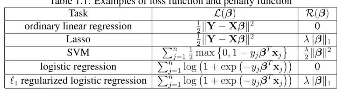
1.1 Examples of loss function and penalty function . . . 3

4.1 Basic algorithm for crime data . . . 72

4.2 Algorithm with inexact iterations for crime data . . . 73

4.3 Basic algorithm fora9a . . . 76

(12)

Chapter 1 Introduction

In this chapter, we first introduce the background of statistical learning in homogeneous models. Then we list applications in which the model is not homogeneous and thus provide motivations for change-points inference in Section 1.1. In Section 1.2, we provide a summary of related works of this thesis. In Section 1.3, we list our main contributions of this thesis. In Section 1.4, we introduce common notations used throughout this thesis. Finally, in Section 1.5, we list the organization of this thesis.

1.1 Background and Motivation

1.1.1 Statistical Learning in Homogeneous Models

Statistical learning in homogeneous models, in which the data is assumed to be generated from a single underlying model, plays a key role in almost every branch in modern science and industry. Here, we give a few real life applications:

• Distinguish cancer versus normal patterns from mass-spectrometric data [1].

(13)

like person’s age, work type, education and capital-gain etc [2].

• Identify relationship between murder rate and community population, per capita income, police operating budget and violent crime rate etc [3].

• Judge whether an email is a spam or not [2].

All these tasks are either linear regressions or classifications. Letndenote the number of sample, pdenote the number of features. For example, for the third task mentioned above, murder rate is the target variable and thus we can use a vectorY ∈Rnto represent

the murder rates ofn given samples. All other variables such as community population, per capita income, police operating budget and violent crime rate can form a matrixX ∈ Rn×p, whose jth row xj ∈ Rp corresponds to jth sample. Thus the problem can be

transformed into a linear regression and the task is to infer the linear relationship between

Y andX, which can be stated as

min β∈Rp 1 2kY−Xβk 2 2, (1.1)

where_k·k2denotes the`2norm. To avoid overfitting and to produce interpretable models,,

usually an`1 penalty is added to (1.1) and thus forms Lasso [4]

min β∈Rp 1 2kY−Xβk 2₊_λ_k_β_k 1, (1.2)

whereλ >0is the regularization parameter, and_{k · k}1denotes the`1 norm.

The other tasks mentioned above are binary classifications which can be done by either support vector machine (SVM) or logistic regression. Since they are binary classification tasks, we can take the positive labels as +1 and the negative labels as ₋1and then we form a label vectorY ∈Rn. AndX ∈Rn×pis formed the same way as linear regression.

(14)

Table 1.1: Examples of loss function and penalty function

Task _L(β) _R(β)

ordinary linear regression 1₂_kY₋Xβ_k2 0 Lasso 1₂_kY−Xβ_k2 λkβ_k1 SVM Pn j=112 max 0,1−yjβTxj λ₂kβk2 logistic regression Pn j=1log 1 + exp −yjβTxj 0

`1regularized logistic regression Pn_j₌₁log 1 + exp −yjβTxj

λkβ_k1

For SVM, we solve the following optimization problem

min β∈Rp n X j=1 1 2max 0,1₋yjβTxj + λ 2kβk 2_, (1.3)

whereyj is thejth element ofY. For logistic regression, we solve

min β∈Rp n X j=1 log 1 + exp ₋yjβTxj . (1.4)

Again to avoid overfitting and produce sparse results, we usually add a `1 norm penalty

as in Lasso to have [5] min β∈Rp n X j=1 log 1 + exp ₋yjβTxj +λ_kβ_k1. (1.5)

In these tasks above from (1.1) to (1.5), our goal is to infer a parameter vectorβ by minimizing a certain function. The optimization problem can be stated as

min

β∈RpL

(β) +_R(β), (1.6) where _L is loss function and _R is penalty function. By adding penalty, the produced models have a certain sparsity structure, which is more interpretable and hence more desirable in practice. Lasso is such an example [4].

(15)

In Table 1.1, we list corresponding_L(β) and_R(β)in the above examples. We in-fer one parameter vector β _∈ _Rp by minimizing the sum of the loss function _L(β) and penalty function_R(β). This implies thatβis same across all the samples. So one under-lying assumption is that the models in the above tasks are homogeneous and all the data samples come from one uniform model, or the model is static. It is reasonable to make this assumption for the examples we mentioned at the beginning of this section. However, as will be discussed in the sequel, it might not be the case for some other applications.

1.1.2 Change-points Inference in Heterogeneous Models

As mentioned above, a typical assumption made in the existing work is that the data come from a single underlying model [4, 6–8]. However, this assumption might not hold in certain dynamic systems.

• In building economic growth models from various indicators, it is more appropriate to assume that the available data obeys different models over different time period as the economic growth pattern undergoes structural changes over the years [9].

• In the analysis of array-based comparative genomic hybridization (array-CGH) data, the underlying model varies in different segments of the DNA sequence [10].

• In the analysis of time dependent Gaussian graphical model, which has wide-spread applications in network traffic analysis and cyber attack detections, the edge struc-ture varies [11].

In all above examples, it is of interest to identify the change-points and build proper mod-els for different regions. This motivates the study change-points inference in statistical models.

For data that come from multiple underlying models, we cannot use homogenous models. Also, since the data are from different models, the learning algorithms in

(16)

homo-geneous models do not work. To address these issues, in this thesis we focus on learning algorithm design and analysis in heterogeneous models.

More specifically, we study the change-points inference problem in this thesis. The change-point identifies the shift point from one model to another. There are two typi-cal formulations for change point problems: online and offline [12, 13]. In the online formulation, the observer receives observations sequentially. And the goal is to design real time algorithms to detect the change in the statistic behavior of the observations. To reduce the computational complexity, a statistic with a recursive form is desirable in the online detection. If such a recursive form exists, the statistic can be updated whenever a new observation arrives. For example, [14] proposes to track the gradual change of en-vironmental parameters, and its statistics are updated recursively by minimizing a regret function.There are many other interesting papers focusing on the online detection prob-lem, such as [15, 16]. In the offline formulation, initiated by [17], the observer is given a complete set of data and the goal is to estimate the location of change-points that segment the data set into several homogenous segments. The offline formulation has also attracted significant research interest (see survey [18] and Chapter 2.6 and 11 of [12]). Here, we list only a few of them to illustrate the its potential applications. For example, a direct application of the offline points estimation is data fitting [19]. The offline change-points estimation is also widely used in economic [20–22], molecular biology [10, 23], and climate data analysis [24].

In this thesis, we focus on the offline formulation with the goal of designing offline algorithms to estimate the location of change-points in a given data set. Since our data set is fixed, we do not focus on the recursive property of our algorithm. Instead, we mainly consider the consistency property and complexity of our estimator. This thesis mainly focuses on offline setting with both low dimensional and high dimensional cases studied. So we divide our work on offline change-points estimation in this thesis based

(17)

on different data dimensions. Next, we introduce three main parts of this thesis on offline change-points estimation.

Thrust 1: Low Dimensional Change-points Inference

We begin by considering offline low dimensional linear regression problems in which the underlying true linear coefficients might undergo multiple changes. Our goal is to esti-mate the number and locations of change-points that segment available data into different regions, and further to produce sparse interpretable models for each region. The problem considered here has been studied extensively in other fields [12], and existing approaches to estimate multiple change-points are mainly based on least-square fitting via dynamic programming (DP) [25–28]. This DP approach will be discussed in detail in Chapter 2.

Although one can also apply the DP approach to solve this problem, there are sev-eral challenges associated with this approach. First, the DP algorithm cannot estimate the number of change-points accurately. It should be noticed that the DP approach needs information about the true number of change-points K∗_{. However,} _K∗ _{in most cases}

are unknown. In particular, if we only know an upper-bound Kmax on the total number

of change-points, then the DP algorithm will always return Kmax change-points. This

is due to by adding new segments, one can always decrease the value of cost function. Hence, the DP algorithm cannot find the true number of change-points unless it is known perfectly. Second, the solution of the DP algorithm does not possess a sparse structure, hence, the model cannot be easily interpreted. Third, the computational complexity of the DP algorithm is high. In particular, for the model with K∗ _{change-points, the}

computa-tional complexity isO(K∗_n3₎_with_n_{being the total number of observations (samples).}

To address these challenges, we propose to solve the change-points estimation prob-lem using sparse group Lasso (SGL), a model fitting method proposed very recently in [29,30]. In SGL, the parameters are divided into groups. There are two penalty terms in

(18)

the SGL problem formulation: thel2 norm penalty, which encourages most of the groups

of the solution to be zero, and the l1 norm penalty, which will promote sparsity within

those non-zero groups. We show that after a proper transformation, the parameters to be estimated possess both inter and intra group sparsity structure. Therefore, after a proper transformation, the problem studied in this thesis fits the scope of SGL and can be solved using SGL. In particular, we reformulate the original linear regression with change-points problem into a convex optimization problem with both l1 andl2 penalties. The solution

of this convex optimization problem then directly provides the number and locations of change-points and the regression coefficients of each region. We prove that, under certain assumptions and a properly chosen regularization weight, the solution of the proposed approach possesses several desirable features: 1) thel2 norm of the estimation errors of

the linear coefficients diminishes as the number of available data increases; 2) the esti-mated locations of the change-points are close to those of the true change-points. We also propose a data-dependent method to choose a proper regularization weight. Further-more, using efficient algorithms for solving SGL problems [30, 31], the complexity of the proposed approach is much lower than that of the DP approach.

Thrust 2: High Dimensional Change-points Inference

There is a growing interest in statistical inference in high dimensional models, in which the number of features or parameters to be estimated pis on the same order of or even larger than the number of data points or observations n, i.e. p_n ₉ 0orp n [32–34]. In this thrust, we focus on change-points estimation in high dimensional linear regression models.

Our goal remains the same as in that of the low dimensional setting. Although the SGL based approach for change-points estimation possesses desirable properties for low dimensional models, the analysis in the low dimensional setting does not apply in the

(19)

high dimensional setting anymore, as it relies critically on the assumption thatpis fixed as n increases. In the high dimensional setting, we develop new tools to analyze the performance of the proposed SGL based approach. The overall strategy of our analysis is to use contradiction. To be more specific, we focus on the difference between the optimal value of the objective function and the objective function evaluated at the true parameters of the model. This difference should always be less than or equal to zero due to the fact that the optimal solution achieves the minimum of the objective function. Suppose some variables satisfying some constraints can be the optimal solution, then if that difference mentioned above is greater than zero, then we form a contradiction. This contradiction means that those constraints do not hold for the optimal solution. Then we can find properties of the optimal solution by reversing those constrains.

Using this strategy, under certain assumptions and using a properly chosen regulariza-tion parameter, we show that the estimaregulariza-tion errors of linear coefficients and change-point locations can be expressed as functions of the number of observations n, the dimension of the model pand the sparse level of the models. From the derived error functions, we can characterize the conditions under which the proposed estimator is consistent.

We further extend our study to general linear models (GLM), which is a broader class of linear models and includes classic models such as logistic regression models. We show that using our approach, if the link function in GLM model is strictly convex, then GLM enjoys the same consistency properties as those of ordinary linear models except for some constant scaling factors. The extension to GLM reveals a broader area of potential applications of the proposed approach.

Thrust 3: Speeding Up Inference Process

Here we consider how to solve change-points estimation problem more quickly. Since we have reformulated the change-points estimation problem as the SGL problem, so here

(20)

we consider how to speed up solving SGL especially for high dimensional data. We are motivated by distributed learning techniques which are increasingly utilized due to the emergence of big data.

For big volume of data, the size of optimization problem is dramatically increasing and hence each machine cannot store all the data. The whole data set is split into parts and each part is stored in one machine. For a machine learning task in this scenario, each machine can only access its local data set and cannot access the whole data set. Since each machine can only store a part of data, the way to partition the whole data set is critical. There two popular ways to partition the data set: partitioning by sample [35] and partitioning by features [36, 37].

In SGL problem formulation, the features of the data are divided into groups. Hence we consider the way of data is storage is partitioning by features. In utilizing distributed learning for speeding up change-points estimation, one of the key steps is to communicate between nodes to update the parameters in the current optimization iteration. The amount of communication has become an bottleneck for speeding up distributed machine learning tasks [35–38]. This motivates us to design communication efficient distributed learning algorithms for feature partitioned data.

One major bottleneck in the design of large scale distributed machine learning algo-rithms is the communication cost. In this thrust, we propose and analyze a distributed learning scheme for reducing the amount of communication in distributed learning prob-lems under the feature partition scenario. The motivating observation of our scheme is that, in the existing schemes for the feature partition scenario, large amount of data ex-change is needed for calculating gradients. In our proposed scheme, instead of calculating the exact gradient at each iteration, we only calculate the exact gradient sporadically. In the iterations when exact gradients are not calculated, we will use the most recently cal-culated gradient as proxy to compute the next update. We provide precise conditions to

(21)

determine when to perform the exact update, and characterize the convergence rate and bounds for total iterations and communication iterations. We further test our algorithm on synthesized and real data sets and show that the proposed scheme can substantially reduce the amount of data transferred between distributed nodes.

1.2 Related Efforts

For low dimensional setting, [14, 39–45], are most relevant to our work. [14] focuses on developing online algorithms to track agradually changingparameter in the environment. Our work, on the other hand, focus on developing offline algorithms to estimate abrupt changes in a given data set. In [39], the authors proposed an adaption of Lasso algorithm to detect changes in the mean value of a sequence of Gaussian random variables and hence the dimension is one. In [40, 41], the authors use group fused Lasso to solve the structural changes in linear regression problems. [42] considers the recovery of models that have multiple types of sparsity structure under a noiseless observation model. As will be clear in the sequel, in our work, two types of sparsity arises only in the transformed domain. This transformation imposes special constraints on the observation matrix, which does not satisfy the assumptions made in [42]. Furthermore, we consider noisy observation model and hence do not aim to recover the underlying signal exactly. [43, 44] discuss change-points detection under a Bayesian setup, i.e., there is a prior distribution on the possible locations of the change points, while this thesis is non-Bayesian. [45] discusses a method to partition observations into different subsets. Similar to [43, 44], the model assumes a prior probability of each partition. Furthermore, the algorithm needs precise knowledge of the distribution of the observations and has a very high complexity (exponential inn). Our work is different from these works in the following aspects. First, we impose an additional sparsity structure in the linear regression coefficient, which is often of interest

(22)

in practice. Hence, instead of group fused Lasso, we use sparse group Lasso to solve the problem at the hand. The additionall1term in our problem formulation brings significant

technical challenges when analyzing the performance of the algorithms. Moreover, we have analyzed the computational complexity of our proposed algorithm, while no such analysis was presented in [40, 41]. We also note that SGL has been used for anomaly detection in smart grid [46].

In addition to the above mentioned work on the change-point estimation in low di-mensional models, our work is also related to existing work on high didi-mensional uniform models [8, 47–51]. [47] discusses the restricted eigenvalue condition in Gaussian design matrices, which is quite useful in high dimensional sparse models. [8, 47, 48] study high dimensional estimation problems under uniform models. In [48], the authors study high dimensional estimation under the sparsity constraint that the parameters are in `q balls.

In [8], the authors show a very general approach to show that, under the assumption that data are from one uniform model, one can prove oracle consistency inequalities in the high dimensional case. In [49], the authors study the change-points detection problem in linear regression with identity design matrices. [50, 51] consider the detection of change-point in high-dimension data using low-dimension compressive measurements in an online set-ting. Our work is different from the works mentioned above in several aspects. First, we consider nonhomogeneous models. Second, we consider high dimensional setting. Third, we require less information about the change-points. For example, we do not need the number of change-points (as required in the DP approach) nor the prior distribution of change-points/partitions (as required in the Bayesian approach).

For speeding up distributed learning, there have been a large number of recent in-teresting works on the sample partition scenario. For example, [52] and [53] proposed Communication Efficient Distributed Dual Coordinate Ascent (CoCoA) algorithm and its variant CoCoA+. In these algorithms, each machine solves a variant of a local dual

(23)

prob-lem and then updates the global parameters at each iteration. [54] designed Distributed Approximate Newton (DANE) algorithm. DANE is suitable for smooth and strongly convex problems and takes advantage of the fact that the subproblems at local machines are similar. In [36], Distributed Self-Concordant Optimization (DiSCO) algorithm was proposed. DiSCO uses an inexact damped Newton method and in each iteration step a distributed version of Preconditioned Conjugate Gradient (PCG) method is used to com-pute the inexact Newton step. In [55–59], variants of stochastic gradient descent (SGD) are proposed.

Compared with the sample partition scenario, the feature partition scenario is rela-tively less well understood. Among limited number of works on the feature partition scenario, in [35, 38], the authors propose to use randomized (block) coordinate descent to solve distributed learning problems for the feature partition scenario. In each iteration, each machine randomly picks a set of coordinates to optimize and apply updates to the parameters and gradients. As pointed out in [35] (will also be discussed in detail in the sequel), the communication cost associated with computing gradients, which are needed to calculate the next update, is very high.

Our work is also related but different from recent interesting work on the design of optimization algorithms with inexact updates. In [60], the convergence rate of inexact update of proximal method is proved. In [61], the optimal trade-off between convergence rate and inexactness is provided. In [62], the authors use an inexact method to solve distributed Model Predictive Control (MPC) problem. In [63], the authors analyze inexact updates in the coordinate descent. The main motivation for these works is to address the case that the subproblem for each machine cannot be solve exactly. In this thesis, however, we assume that each subproblem can be solved exactly and we try to introduce inexact updates or approximations to reduce communication cost. Our works is different from the works mentioned above in several aspects. First, this thesis focuses on feature partitioned

(24)

data. Second, we use inexact updates to reduce communication cost, not based on the assumption that subproblem at each machine cannot be solved exactly. Third, we take a deterministic approach.

1.3 Contributions

We begin our work by studying multiple change-points estimation in low dimensional linear regression models. In this part, we list our contributions as follows [64].

• We transform the multiple change-points estimation problem into an SGL problem.

• We prove that the solution enjoys desirable properties: the estimation errors of the linear coefficients diminishes as the number of available data increases; the estimated locations of the change-points are close to those of the true change-points.

• We show that the complexity of the proposed approach is much lower than that of the DP approach.

Then we extend our results to high dimensional setting [65].

• We show that the estimation errors of linear coefficients and change-point locations can be expressed as functions of the number of observations n, the dimension of the modelpand the sparse level of the models.

• We can characterize the conditions under which the proposed estimator is consis-tent.

• We further extend our method to generalized linear models (GLM) and prove more general results.

For speeding up computation using distributed learning, we have the following contribu-tions [66].

(25)

• We propose a communication efficient distributed learning algorithm to speed up a wide class of learning problems.

• We provide analytical results of communication amount of the proposed algorithm.

• We provide several practical techniques and simulations to show its feasibility in practice.

1.4 Notation

Here we introduce the notation convention used throughout this thesis. We use upper case boldface letters (e.g.,X) to denote matrices and lower case boldface letters (e.g.,x) to denote column vectors. For a matrix X, we useXi,_· to denote theith row of X, and use X_·,j to denote the jth column ofX. For a positive integerk, we use[k] to denote {1,2,· · · , k}. We define[b, e] := {b, b+ 1,· · · , e}whereeandbare integers withe≥b. Similarly,[b, e) :={b, b+ 1,· · · , e−1}. We use_Rto denote the set of real number. Letf

be a function, we use_∇f(x)to denote the gradient off atx. We usec,c0 andc1, c2,· · ·

to denote positive constants.

1.5 Roadmap

Chapter 2 begins by introducing our problem formulation in low dimensional linear re-gression models. Then we show how to transform the multiple change-points estimation problem into an SGL problem. Theoretical guarantees are provided for the results of our approach. We provide simulation results of our approach.

Chapter 3 begins by extending our approach in low dimensional linear regression models to high dimensional linear regression models. Then we provide theoretical results for characterizing the estimation errors in expression of number of observations n, the

(26)

dimensionpand the sparse levels. Using these theoretical results, we can find the growth order of n, p and s to get a consistent estimator. We further extend our approach to GLM and prove corresponding analytical results, which implies our approach has a wide application range in practice.

Chapter 4 begins by introducing the concerns of high dimensional data which needs huge amount of computation power for change-points inference and other similar ma-chine learning tasks. Hence we consider utilizing distributed learning. We propose a communication efficient distributed learning algorithm and propose analytical results for the amount of communication. Furthermore, we show how to set the parameters in the algorithm and show performance of our algorithm in practice.

Chapter 5 concludes the dissertation. It outlines the contributions of the dissertation and summarizes the thesis statement of this work.

(27)

Chapter 2 Low Dimensional Change-points

Inference

This chapter begins the main part of this thesis by focusing on change-points inference in low dimensional linear regression models. In Section 2.1, we describe the model under consideration. In Section 2.2, we describe the proposed SGL based approach. In Section 2.3, we prove the consistency of the solution of our approach. In Section 2.4, the com-plexity of SGL algorithm is discussed. In Section 2.5, we provide numerical examples to validate the theoretic analysis.

2.1 Model

We consider the linear regression model

yt=β∗tTxt+t, t∈[n], (2.1)

wherextis apdimensional vector,β∗_t is apdimensional sparse coefficients vector, where

(28)

and identically distributed (i.i.d.) with_N(0, σ2₎_{. Here}_N₍₀_{, σ}2₎_{is the probability density}

function (pdf) of Gaussian random variables with zero mean and varianceσ2_.

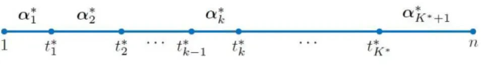
We consider the scenario that the values ofβ∗_t’s change over time. In particular, we assume that the linear model experiences K∗ _{times of changes in the values of} _β∗

t’s,

and the set of change time instances (or change-points) are denoted as T∗ ₌ _{_t∗

k, k =

1, . . . , K∗_}_{. Hence, for}₁_≤_k_≤_K∗_{+ 1}_{, we denote}

β∗_t =α∗_k, fort∗_k₋₁ ≤t ≤t∗_k−1, andα∗_k₆=α∗_k₋₁,

wheret∗

0 = 1andt∗K∗₊₁ = n+ 1by convention, and{α∗_k, k = 1,· · · , K∗}are the true

values of coefficients, which are fixed but unknown. Our goal is to estimate the change-points _{t∗_k}_{, the coefficients}_{_α∗_k} _{and the number of change-points}_K∗ _through_n _pairs

of observed data(xt, yt). Figure 2.1 illustrates the model.

Figure 2.1: Illustration of model.

LetKmaxbe a known upper bound on the number of change-points andKmax << n,

then the multiple change-points estimation problem can be written as

min β 1 n n X t=1 (yt−βTtxt)2, s.t. n−1 X t=1 1{β_t₊₁ ₆=β_{t} ≤}Kmax, (2.2)

where1{·}is the indicator function, whose value is0ifβ_t₊₁ =β_tand is1otherwise. An intuitive approach to solve (2.2) is the exhaustive search, in which one solves a

(29)

least square fitting problem for each possible change pattern, and picks the solution with the least residual square error. However, the total number of possible change patterns is PKmax K=0 n K

, which results in an extremely high computational complexity.

A more efficient way to solve (2.2) is to use DP as described below. Note that the the-oretical analysis follows directly from discussion in [28], and the pseudocode is revised from DP algorithm in [67]. Let _MK,n be the set of all segmentations with K

change-points (K + 1segmented intervals) up tonth sample. Letrk(m) = [tk, tk+1)be thekth

interval of segmentationmdelimited by change-pointstk andtk+1. Any segmentationm

of _MK,t can be written as _{[t0, t1),· · · ,[tK, tK+1)} = {r0(m),· · · , rK(m)} with

con-vention t0 = 1 and tK+1 = n + 1. Then our task is to find an optimal segmentation

m _{∈ MK,n} to minimize to total cost. Our problem is to solve

min m∈MK,n ( X r∈m min α∈Rp ( X i∈r (yi−αTxi)2 )) .

For any segmentr, we define the cost asgr(α) =P_i_∈_r(yi−αTxi)2 and the optimal

cost ascr= minα∈Rpgr(α). LetCK,n = minm∈MK,n P

r∈mcr . So we can retrieve the

update equation

∀t_≥K CK,t = min

K−1≤j≤t−1

CK−1,j+c[j+1,t] . (2.3)

CPE DP solves multiple change-points estimation problem using DP, and PRINT SOLUTION reconstructs and prints the solution.

(30)

Algorithm 1CPE DP(X,Y,p,n,K∗)

letr[0_{· · ·}K∗_,₁_{· · ·}_n_]_{be a new matrix and}_s_[1_{· · ·}_K∗_,₁_{· · ·}_n_]_{be a new matrix}

fort = 1tondo r[0, t] =c[1,t] end for forK = 1toK∗ _do fort=K tondo q =_∞ forj =K₋1tot₋1do ifq > r[K−1, j] +c[j+1,t]then q=r[K₋1, j] +c[j+1,t] s[K, t] =j+ 1 end if end for r[K, t] =q end for end for returnrands

Algorithm 2PRINT SOLUTION(X,Y,p,n,K∗)

(r, s)= CPE DP(X,Y,p,n,K∗₎ K =K∗ whileK >0do Prints[K, n] n =s[K, n] K =K−1 end while

(31)

complexity to computec[j+1,t]isΘ(t−j), then K∗ X K=1 n X t=K t−1 X j=K−1 (t₋j) = K∗ X K=1 n X t=K (t₋K+ 2)(t₋K + 1)/2 = K∗ X K=1 ((n₋K)(n₋K+ 1)(2n₋2K + 1)/12 + 3(n₋K)(n₋K+ 1)/4 +n₋K).

From analysis above, we know the complexity of DP approach isΘ(K∗_n3₎1_.

Here we list two more drawbacks of this approach. First, the time complexity of DP approachΘ(K∗n3₎_{is still very high especially when}_n _{is large. Second, the solution of}

DP is not sparse in the sense that the estimated βˆ_ts are not sparse vectors, which is not desirable when the interpretability of the model is important.

Motivating by the challenges of exhaustive search and DP approaches, we propose the SGL based approach for the proposed change-point estimation problem, which is described in the following section in detail.

2.2 Proposed SGL Based Approach

Letθ∗₁ =β∗₁andθ∗_t =β∗_t₋β∗_t₋₁fort= 2,_{· · ·}, n. Furthermore, letβ∗ = (β∗₁T,β₂∗T,_{· · ·} ,β∗_nT)T_,

θ∗ = (θ∗₁T,θ∗₂T,_{· · ·} ,θ∗_nT)T_{. Notice that both}_β∗ _and_θ∗ _are_np_{dimensional column}

vec-tors. From Section 2.1, we observe that most of θ∗_t are zero vectors (there are at most

Kmax nonzeroθ∗t vectors). Furthermore, for those non-zeroθ∗t’s, most of the entries in

1_{Throughout the thesis,}_o

p(f(n)) =g(n)means thatlimn→∞P(|f(n)/g(n)|> ) = 0for any >0;

Op(f(n)) =g(n)means that for any >0, there exists a finitec >0such thatP(|f(n)/g(n)|> c)< for anyn;o(g(n)) =f(n)means that for any positive constantc >0, there exists a constantn0>0such that0_≤f(n)< cg(n)for alln_≥n0;O(g(n)) =f(n)means that there exist positive constantscandn0 such that0_≤f(n)_≤cg(n)for alln_≥n0;Θ(g(n)) =f(n)means that there exist positive constantsc1,

c2, andn0such that0≤c1g(n)≤f(n)≤c2g(n)for alln≥n0;Ω(g(n)) =f(n)means that there exist positive constantscandc0such that0≤cg(n)≤f(n)for alln≥n0.

(32)

θ∗_t are zero, asβ∗_t’s are sparse vectors. As the result, if we view θ∗_t’s as groups within

θ∗, thenθ∗ has the following group sparse structure: most of the groups are zero, and for those non-zero groups, most of the entries within the group are zero.

LetY = (y1, y2,· · · , yn)T,e= (1, 2,· · · , n)T and X =          xT 1 xT 2 · · · xT n          , ˜ A =          Ip Ip Ip · · · · Ip Ip _{· · ·} Ip          ,

whereIp is the identity matrix of sizep×p. HenceYandEare vectors ofndimension,

andXandA˜ are matrices of sizen_×npandnp_×np, respectively. Define

˜ X=XA˜ =             xT 1 xT 2 xT2 xT 3 xT3 xT3 · · · · xT n · · · xTn             , (2.4)

then, it is easy to verify that our model can be rewritten as

Y =Xβ∗+e= ˜Xθ∗+e. (2.5) To obtain the estimates of the number and locations of change-points and linear

(33)

coeffi-cients of each region, letβ₀ =0p_×1, we propose to solve min β 1 nkY−Xβk 2 2+γλn n X t=1 kβ_t₋β_t₋₁_k₂ +(1₋γ)λn n X t=1 kβ_t₋β_t₋₁_k1, (2.6)

which can also be rewritten as

min θ 1 nkY−X˜θk 2 2+γλn n X t=1 kθtk2+ (1−γ)λnkθk1, (2.7)

where_k·k2is the`2norm,k·k1is the`1norm,λnis the regularization penalty weight, and γ _∈(0,1)adjusts the relative weight for the two penalty terms.γaffects the inter and intra group sparsity of the solution obtained from this optimization problem. The inter group sparsity is increased when we increaseγ, while the intra group sparsity is increased when we decreaseγ. Theoretically, as we can see from Proposition 1 and Proposition 2, as long as γ is a constant in(0,1), we will have the consistent results in the change-point and coefficient estimations under proper assumptions. In practice, the choice of γ depends on the application. If one expects a strong group-wise sparsity, one should select γ to be a larger constant. If, in other applications, one expects mild group-wise sparsity, one should choose γ to be a smaller constant. We will discuss how to choose λnin Section

2.3. We note that the proposed problem formulation and algorithm do not depend on the parameterKmaxor knowledge ofK∗.

Notice that problem (2.7) is of the form of SGL proposed in [30]. As illustrated in [30], the penalty term Pn

t=1kθtk2 encourages the group-wise sparsity, which implies

that in the solution of (2.7) most ofθts are zero vectors, while kθk1 encourages sparsity

within each group, which implies that in the solution of (2.7) most of entries are zero for those nonzero vectors. We also notice that (2.7) is a generalization of the problem

(34)

considered in [41], in which a particular case withγ = 1andp= 1is considered.

Let _{θˆ_t}, _{βˆ_t}, Kˆ and Tˆ_kˆ = {ˆtk, k = 1,· · · ,Kˆ} denote estimates of {θt}, {βt}, K∗ and T∗, respectively. For a given solution _{θˆ_t} of (2.7), we can obtain _{βˆ_t} from the linear relationship between θ and β. We can treat the nonzero vectors among θˆ_t’s as change-points, from which the estimate of the total number Kˆ and locations Tˆ_kˆ =

{tˆk, k = 1,· · · ,Kˆ}of the change-points can be determined.

For1_≤k_≤Kˆ + 1, we denote

ˆ

αk = ˆβt, fortˆk−1 ≤t≤tˆk−1, andαˆk 6= ˆαk−1.

By convention, we settˆ0 = 1andˆt_Kˆ₊₁ =n+ 1.

2.3 Consistency

In this section, we study the properties of the solution of our SGL based approach (2.7). We provide consistency results and discuss how to choose the regularization parameter

λnproperly.

To assist the following presentation, we define

Imin = min 1≤k≤K∗|t ∗ k+1−t∗k|, (2.8) Jmin = min 1≤k≤K∗kα ∗ k+1−α∗kk2. (2.9)

Hence, Imin is the minimal interval between two consecutive change-points, andJmin is

the minimal`2 distance between two consecutive true different coefficient vectors.

Let_{δn}be a sequence of positive quantities that decrease to zero asn→ ∞. Letxt,m

(35)

A1: 0 < l_≤ inf 1≤s<r≤n+1 r−s≥nδn µmin 1 r−s r−1 X t=s xtxTt ! ≤ sup 1≤s<r≤n+1 r−s≥nδn µmax 1 r₋s r−1 X t=s xtxT_t ! ≤L <_∞,

as n → ∞, whereµmin(·)and µmax(·)are the minimum and maximum eigenvalue of a

matrix respectively.

Intuitively, A1 means that the eigenvalues of the averaged matrix _r₋1_sPr−1

t=s xtxTt

are bounded, which indicates thatxtxTt is a well behaved matrix.

A2: Imin/(nδn)→ ∞, asn → ∞.

A2 sets a requirement on the minimum intervals between any two consecutive change-points. In particular, we requireImin to grow asngrows. This assumption is reasonable

as ifImin does not increase whenn increases, then there exists an interval whose length

is diminishingly small compared ton. It will be challenging to identify this interval from the whole data sequence.

A3: _∀1_≤m_≤p,_∀1_≤s < r_≤n+ 1andr₋s _≥nδn, lnn (r₋s)2 r−1 X t=s x2_t,m/J_min2 _→0. x2

t,m can be viewed as the power of the mth dimension of xt. Intuitively speaking, A3

implies that Jmin, the minimal`2 distance between two consecutive true different

coef-ficient vectors, cannot be too small. This is a reasonable assumption, as if Jmin is too

small, there exists a change point at which the coefficient changes very little. It will be challenging to detect such as a change.

Proposition 1. Under A1-A3, if Kˆ = K∗_{, and we choose}_λ

(36)

n → ∞, then P max 1≤k≤K∗ ˆt_k−t∗_k ≤nδ_n →1, as n → ∞. (2.10) Proof. Please see Appendix A.2.

Proposition 2. Under A1-A3, if Kˆ = K∗_{, and we choose}_λ

n such that _J_minλn_δ_n → 0 as n _{→ ∞}, then kα∗_k₋αˆ_kk2 ≤ nλn(γ+ (1−γ)√p) +IminoP(Jmin) (Imin−2nδn)l , (2.11) in probability asn_{→ ∞}, for_∀1_≤k _≤K∗_{+ 1}_.

Proof. Please see Appendix A.3.

As discussed above,K∗ _{is the true number of change-points, which is assumed to be}

a constant. Furthermore, from A2, we know thatImin is assumed to be sufficiently large,

which implies thatK∗_{cannot be arbitrarily large.}

Remark 1. Propositions 1 and 2 indicate that the proposed SGL based algorithm can lead to consistent estimations of the change-points and the linear coefficients. Proposition 1 is easy to interpret: from A2, we know thatnδn/Imin →0, which implies that the maximum

relative change-points location estimate error is diminishing. Proposition 2 is a little complicated. Actually, there are several combinations of Imin, Jmin that can make the

estimation of the linear coefficients consistent. For example, ifImin = Θ(n)andJmin is

a constant, then as long asλn→0, we havekαk−αˆkk2 →0. To see this, we first notice

thatIminoP(Jmin)/((Imin−2nδn)l)→0. Moreover,

nλn(γ+ (1−γ)√p) (Imin−2nδn)l = λn δn γ+ (1−γ)√p (Imin/(nδn)−2)l → 0 (2.12)

(37)

Proposition 2 and Jmin being a constant mentioned above) and Imin/(nδn) → ∞ as

indicated in A2.

Remark 2. Due to the special structure ofX˜ as shown in(2.4), we cannot directly apply the existing bounds on the performance of regularized M-estimator (see, e.g., [8]). Hence we need a different approach to bound thel2norm of the error in the proof of Proposition

2.

The above results require Kˆ = K∗_{. In the following, we show that even if this}

assumption does not hold, we can still guarantee certain accuracy of the estimated change-points. For two sets_S1 andS2, we define

ε(S1||S2) = sup

s2∈S2

inf

s1∈S1|

s1−s2|. (2.13)

Notice thatmax_{ε(S1||S2), ε(S2||S1)}is the Hausdorff distance betweenS1 andS2 [68].

Since_Tˆ_Kˆ andT∗ are the set of estimated change-points and the set of true change-points

respectively, so they can be written as

ˆ

T_Kˆ := ˆt1,tˆ2,· · · ,ˆt_Kˆ ,

T∗ := {t∗1, t2∗,· · · , t∗K∗}.

Using this notation, Proposition 1 can be restated as thatε(ˆTK||ˆ T∗)≤nδnandε(T∗||Tˆ_Kˆ)≤

nδnhold at the same time in probability asn→ ∞whenKˆ =K∗. The following

propo-sition is parallel to Propopropo-sition 1 for the caseK∗ _<_{K < K}ˆ

max.

Proposition 3. Under A1-A3, and chooseλn such that _J_minλn_δ_n → 0 asn → ∞, then if K∗ _<_Kˆ _≤_K_max_{, we have}

(38)

Proposition 3 implies that, if the number of the change-points is overestimated, i.e.

ˆ

K > K∗_{, then there exists at least one estimated change-point falling in the range} _nδ

n

of each true change-point. In the following, we show that the event_{Kˆ ≥ K∗}happens with a large probability.

We define Imax = max 1≤k≤K∗|t ∗ k+1−t∗k|, Jmax = max 1≤k≤K∗kα ∗ k+1−α∗kk2,

and we impose another assumption:

A4. Imin = Θ(n);Jmax =O(1);Jmin = Ω(1).

Proposition 4. Under A1-A4, and we chooseλnsuch that _J_minλn_δ_n →0asn→ ∞, then

P( ˆK ≥K∗)→1, as n→ ∞. (2.15)

Remark 3. With A4, the conclusion of Proposition 2 can be further simplified. Notice that Jmax = O(1) indicates oP(Jmin) → 0. Moreover, A2 and _J_minλn_δ_n → 0 indicates

nλn

IminJmin → 0, which further indicates

nλn

Imin → 0 as Jmin ≤ Jmax. Therefore, we can conclude

nλn(γ+ (1−γ)√p) +IminoP(Jmin)

(Imin−2nδn)l →

0.

That is, Kˆ = K∗ _{with A1-A4 can guarantee the estimations of linear coefficients are}

consistent.

(39)

such that λn

Jminδn → 0, we will have either: 1)

ˆ

K = K∗, in which case we have Propo-sitions 1 and 2 for the consistency of the estimates; or 2) K > Kˆ ∗, in which case, we have Proposition 3 for the consistency of the estimates. However, ifK < Kˆ ∗, then some change-points are not detected. Hence it is more desirable to haveKˆ _≥K∗_.

If one insists on having Kˆ = K∗_{, we have the following data-dependent method to}

choose λn. This approach is based on the Akaike information criterion (AIC) [69]. For

any givenλn, we first solve (2.7) and obtainKˆ andTˆ_Kˆ ={ˆtk, k= 1,· · · ,Kˆ}that divides

the data intoKˆ + 1regions. We define

B( ˆT_Kˆ) = 1 n ˆ K+1 X k=1 ˆ tk−1 X t=ˆtk−1 (yt−αˆTkxt)2, (2.16)

whereαˆkis the ordinary least squares (OLS) estimator in the interval[tk−1, tk−1].

Then we propose to minimize the cost function

C(λn) = ln(B( ˆT_Kˆ)) +ρnp( ˆK+ 1), (2.17)

whereρn is a designed parameter such thatρn → 0and _δρ_nn → ∞asn → ∞. In (2.17),

ln(B( ˆT_Kˆ))measures the accuracy of how well the model is fitted, andρnp( ˆK+ 1)is the

penalty of the number of estimated change-points.

Denote Ω = [0, λmax], in which λmax is the maximum value of λn such that the

solution to (2.7) is not all zero vectors. λmaxcan be easily computed. Define

Ω₋ =_{λn∈Ω|K < Kˆ ∗},Ω+ ={λn∈Ω|K > Kˆ ∗},

andλ∗ _{is any}_λ

nsuch thatKˆ =K∗.

(40)

Proposition 5. Under A1-A4, and λn Jminδn →0, we have P inf λn∈Ω+∪Ω− C(λn)> C(λ∗) →1, as n _{→ ∞}.

Remark 5. Proposition 5 provides a method to choose the regularization parameterλn

to guarantee the stronger result. In particular, if we chooseλn = λ∗ and use this value

in (2.7), then we have Kˆ = K∗ _{with probability}₁_{. On the other hand, if one does not}

insist in havingKˆ =K∗,λncan be simply chosen to satisfyλn/(Jminδn)→0. Any value

satisfying this condition will guarantee that the consistent results in Propositions 1_∼ 4 hold.

Remark 6. If we set p = 1, the problem considered in this thesis becomes a basic To-tal Variance (TV)-regularization problem [70–72]. By settingp = 1in the propositions above, we have the consistent results for this special case. Note that these results do not mean that we obtain full understanding of the TV-regularization problem. They simply imply that for the basic TV-regularization problem, we have certain consistency results regarding the change-points estimations and coefficient estimations under the assump-tions made in this thesis.

2.4 Complexity

In this section, we study the computational complexity of SGL algorithms. Denote the cost function in (2.7) as φ(θ) = 1 n Y− ˜ Xθ 2 2+γλn n X t=1 kθ_ik₂+ (1−γ)λn n X t=1 kθik₁, (2.18)

(41)

In our model, we have ann ×1 output vector Y, an n×np data matrix X˜ which can be divided into n sub-matrices, X˜(1)_,_{· · ·} _,_X˜(n)_{, and each} _X(t) _{is an} _n _×_p _matrix

for t = 1,· · · , n, and an np×1coefficient vector θ which can be divided inton p×1

sub-vectors,θ₁,_{· · ·} ,θ_n. The cost function (2.18) can be rewritten as

φ(θ) = 1 n Y₋ n X t=1 ˜ X(i)θ_i 2 2 +γλn n X t=1 kθ_ik₂+ (1−γ)λn n X t=1 kθ_ik₁, (2.19) andX˜(i) ₌ 0p×1 · · · 0p×1 xi · · · xn T .

We define another function which will be used in further analysis. Define

φinner(θk) = 1 n r(−k)−X˜ (k)_θ k 2 2+γλnkθkk2 +(1−γ)λnkθkk1+φother(k), (2.20) where r(₋k) = Y ₋ Pn t=1,t6=kX˜(t)θt and φother(k) = γλn Pn t=1,t6=kkθik2 + (1 −

γ)λnPn_t₌₁_,t₆₌_kkθik₁. φinner(θk) is a function of coefficients of groupk while keeping

the coefficients of other groups as constants.

First, we discuss a modified version of SGL algorithm in [30]. We only describe an outline of the algorithm whose details can be found in [30]. For any given λnandγ, the

(42)

Algorithm 3SGL RBCD(X,Y,p,n) initializeθto be anp_×1zero vector

r =Y₋Pn

t=1X˜(t)θt

repeatpickk= 1,· · · , nwith probability 1_n .outer Loop

r(−k) = r+ ˜X(k)_θ

k

if the optimal coefficients of groupk are identically zerosthen

θnew_k = 0

else

initializeθnew_k (0)to be ap_×1zero vector

i= 0

repeati=i+ 1 .inner Loop

θnew_k (i) = U(θnew_k (i−1)) untilconvergence θnew_k =θnew_k (i) end if r =r+ ˜X(k)₍_θ k−θnewk ) θold_k =θk θk =θnewk untilconvergence returnθ

In this algorithm, we have an outer loop which iterates over all groups until conver-gence, and an inner loop which calculates the optimal coefficients of a particular group while the coefficients of other groups are viewed as constants. The functionU in the in-ner loop is the update function. The function U takes in the old coefficients of group

k θnew_k (i ₋1) and output the new coefficients of group k θnew_k (i) until convergence. The function U can be viewed as a black box. For completeness, we expand U as its

(43)

simplified form in [30]. Let S(·) be the coordinate-wise soft thresholding operator and

(S(z, b))j := sign(zj)(|zj| −b)+, wherez is a vector, b is a scalar and (S(z, b))j is the jth element of the output vector ofS(·). Letl(r(−k),θk) = _n1

r(−k)−X˜ (k)_θ k 2 2 be the

unpenalized loss function. Then the functionU is defined as

U(θk) = 1− tγλn S(θ_k−t∇l(r₍₋_k₎,θ_k), t(1−γ)λ_n) 2 ! + S(θk−t∇l(r(−k),θk), t(1−γ)λn),

wheretis the step size of the gradient method.

The “convergence” is the termination condition, e.g.,_kθnew_k (i)₋θnew_k (i₋1)_k2 < ,

|φ(θnew_k )₋φ(θold_k )_| < , etc. In the original algorithm proposed in [30], the outer loop is chosen in a cyclical order. Since the convergence rate of cyclically block-coordinate descent method is unknown except for some special cases [73], in the algorithm described above, we modify the outer loop of algorithm in [30] to the randomized block-coordinate descent (RBCD) method in [74]. We will use Algorithm 2.4 in our simulation.

Although Algorithm 2.4 is easy to implement, it is difficult to analyze its complexity due to its inexact nature of the inner loop. In the following, we introduce the modified Signed Single Line Search (SSLS) algorithm in [31], which is more amenable to com-plexity analysis.

(44)

Algorithm 4SSLS RBCD(X,Y,p,n) initializeθto be anp_×1zero vector

r =Y₋Pn

t=1X˜(t)θt

repeatpickk= 1,· · · , nwith probability 1_n .outer Loop

r(−k) = r+ ˜X(k)_θ

k

θnew_k =argmin_θ

k{φinner(θk)} .inner Loop

r =r+ ˜X(i)₍_θ

k−θnewk )

θk =θnewk

untilconvergence returnθ

The original SSLS algorithm has a similar structure as the SGL algorithm in [30]. In the description above, we make the same modification, i.e., change the cyclical order to random order in the outer loop. The main difference between Algorithm 2.4 and 2.4 lies in the inner loop. In the inner loop, SSLS explicitly solves the optimal group coefficients for one group while keeping the coefficients of other groups as constants. The main result is in the following Proposition.

Proposition 6. For an error toleranceand a given constant confident level ρ _∈ (0,1), the complexity of the randomized block-coordinate descent method version of SSLS for the worst case isO(n2_λ−2

n )that guarantees

P(φ(ˆθ)₋φ∗ _≤)_≥1₋ρ. (2.21) Proof. Please see Appendix A.7.

The complexity relies onλn. For example, ifλn= √_ln1_n andδ= √31

lnn, a valid choice

for Proposition 1-4 under A1-A4, then the complexity is O(n2_ln_n₎_{, which is better than}

(45)

2.5 Numerical Results

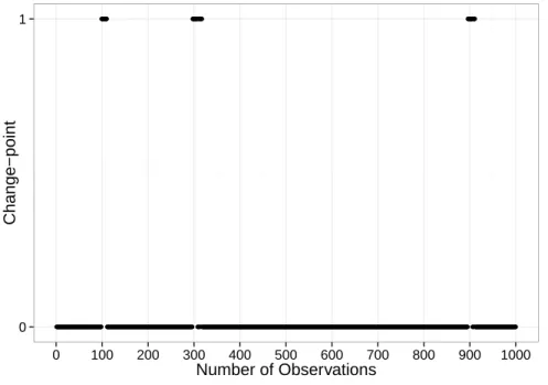
Our simulation is based on the Algorithm 1, a slightly modified version of the algorithm in [30] that has an R implementation in the package SGL. We first test our algorithm on synthesised data. We selectp= 20, and set the number of nonzero coefficients to be4. In particular, we set the first four coefficients to be nonzero in eachβ_t. In our simulation, we

set γ = 0.927, n = 1000,K∗ = 3, and the real change-points are at100,300,900. The

first four coefficients ofβ_ts are all2for pointst = 1,· · · ,99and fort = 100,· · · ,299, and are all ₋2for t = 300,_{· · ·} ,899 and fort = 900,_{· · ·},1000. Eachxt,m ∼ N(0,4),

and the noiset∼ N(0,0.01).

In our simulation result figures, x-axis represents the locations from1ton, and y-axis represents whether the data point at each location is an estimate change-point (1 means that it is an estimated change-point, i.e.,θˆt 6=0, while0meansθˆt=0.).

0 1

0 100 200 300 400 500 600 700 800 900 1000

Number of Observations

Change−point

Figure 2.2: Change-points locations estimation using SGL,λ = 0.003778942.

(46)

Further-more, the nonzero vectors are clustered around the true change-points. This implies that our approach can successfully identify the locations of change-points.

We also examine the regularization path ofθˆ300by choosing different values ofλn. If

we selectλnlarge enough, then the penalty term will dominate the SGL and encourages

the sparsity, thus the coefficients are tending to be all zeros. If we decreaseλn, the least

square term becomes more and more dominant, thus the sparsity of coefficients will de-crease. On the other hand, from our asymptotic results, we know that the accuracy will increase. Hence, in practice, we need to setλnproperly to balance between accuracy and

sparsity. From regularization path, we find that onceλnis properly chosen, our algorithm

can properly identify the important coefficients.

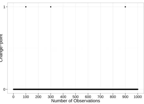
Here we compare our approach with the DP based approach. Figure 2.3 illustrates the estimated change point using the DP based approach when Kmax is set to be 3, the

true value of K∗_{. It shows that the change-points location estimates are accurate if we}

know K∗_{. However, as discussed in Section 1.1.2, if} _K∗ _{is unknown and only} _K max

is known, the DP based approach will return Kmax change-points. Figure 2.4 shows

the change-points estimates using the DP based approach when Kmax is set to be 20.

From the figure, we can see that the returned change-points estimates do not concentrate around the true change points and hence do not provide accurate estimates of the true underlying change-points. Furthermore, the coefficients of all the results by DP approach do no possess sparse structure, which means that most or even all of the coefficients are nonzero while the results of our SGL based approach possess sparsity.

Next, we test our approach on real weather data collected by NOAA. We use NCEP/NCAR Reanalysis 1 Surface Monthly Mean dataset [75]. The dataset records monthly means of precipitation for 1948-present for all locations on the globe, and each locations has

2.5◦ _× ₂_.₅◦ _{resolution. Our goal is to find change-points in climate models for}

(47)

0 1

0 100 200 300 400 500 600 700 800 900 1000

Change−point

Figure 2.3: Change-points locations estimation using DP,Kmax= 3.

South Africa and India because of their diverse geological properties. The parameters of these target locations are considered as Yin our model. Then we pick 40locations near the target locations as the _{xt_} in our model. For each location, we pick the first 400

data. Then we concatenate the dataY and_{_xt}for different locations. Hence, we have

n = 5×400 = 2000andp = 40. And in our concatenated data, the first segment, i.e.,

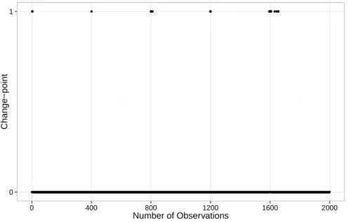
1≤n ≤400, the model describes the relationship between Eastern USA and our40data locations, the second segment, i.e.,401 _≤n _≤ 800, the model describes the relationship between Brazil and our40data locations, and so on. We choose the precipitation as the parameter to be investigated in the model, andγ = 0.8634729in our simulation.

Figure 2.5 shows thel1norm of our result. From Figure 2.5 we can see the inter-group

sparsity of the result. Furthermore, the estimated change-points are clustered around the true change-points.We also examine the regularization path. For the first estimated interval, whenλ = 0.01267545, coefficients at indices9−16and25−32are zero, that is

(48)

0 1

0 100 200 300 400 500 600 700 800 900 1000

Change−point

Figure 2.4: Change-points locations estimation using DP,Kmax = 20.

16coefficients out of40are zero, which show the sparsity within the group. Furthermore, these coefficients corresponds to locations near eastern US, western US and India. Since the data inY of segmentn= 1ton= 400is from eastern US, the result above indicates that precipitation of eastern US has a higher correlation with precipitation of locations near eastern US, western US and India than precipitation of Brazil and South Africa, since eastern US, western US and India are all located in northern hemisphere and near heavily rained regions which is consistent of [76].

(49)

0 1

0 400 800 1200 1600 2000

Change−point

(50)

Chapter 3 High Dimensional Change-points

Inference

In this chapter, we extend our analysis in low dimensional linear regression models to high dimensional setting and further extend it to GLM. In Section 3.1, we describe the model under high dimensional setting. In Section 3.2, we prove the consistency and properties of the solution of our approach. In Section 3.3, we extend our study to generalized linear models. In Section 3.4, we provide numerical examples to illustrate the performance of our approach.

3.1 Model

3.1.1 Problem Formulation

Here we consider the linear regression model in (2.1). Since this section focuses on high dimensional case, hereβ∗_t _∈_Rpis a sparse coefficients vector with sparse levelsandp/n

does not go to zero asn_{→ ∞}.