Large-Scale Vector Data Visualization Using
High Performance Computing
Ahmed S. Ali, Ashraf S. Hussein and Mohamed F. Tolba
Faculty of Computer and Information Sciences, Ain Shams University, Cairo, Egypt
email :{[email protected], [email protected], [email protected]}
Ahmed H. Yousef
Faculty of Engineering, Ain Shams University, Cairo, Egypt
email: [email protected]
Abstract —In computational flow visualization, integration based geometric flow visualization is often used to explore the flow field structure. A typical time-varying dataset from a Computational Fluid Dynamics (CFD) simulation can easily require hundreds of gigabytes to even terabytes of storage space, which creates challenges for the consequent data-analysis tasks. This paper presents new techniques for visualization of extremely large time-varying vector data using high performance computing. The high level require-ments that guided the formulation of the new techniques are (a) support for large dataset sizes, (b) support for temporal coherence of the vector data, (c) support for distributed memory high performance computing and (d) optimum utilization of the computing nodes with multi-cores (multi-core processors). The challenge is to design and implement techniques that meet these complex requirements and bal-ance the conflicts between them. The fundamental innova-tion in this work is developing efficient distributed visualiza-tion for large time-varying vector data. The maximum per-formance was reached through the parallelization of mul-tiple processes on the mulmul-tiple cores of each computing node. Accuracy of the proposed techniques was confirmed compared to the benchmark results. In addition, the pro-posed techniques exhibited acceptable scalability for differ-ent data sizes with better scalability for the larger ones. Finally, the utilization of the computing nodes was satisfac-tory for the considered test cases.
I. INTRODUCTION
The massive progress in high performance computing resources enabled the simulation of complex phenomena in unprecedented details. Examples include data from the study of weather forecasting, crash simulation, crack propagation in a material, unsteady flow surrounding flying vehicles, seismic signals from geological strata, and the merging of galaxies. A typical time varying data-set from a Computational Fluid Dynamics (CFD) simula-tion can contain hundreds of time steps, and each time step can have more than millions of data points. General-ly, multiple values are stored at each data point. As a re-sult, some datasets can easily require hundreds of giga-bytes to even teragiga-bytes of storage space, which creates
challenges for the consequent data analysis tasks. When scientists attempt to visualize and understand the data generated from simulations, the huge size of the data is one of the major challenges. To address these challenges, a lot of research work has been pursued [1, 2, 3, 4] focus-ing on large scale data visualization. However, most of the techniques were developed for the visualization of scalar data [4].
Visualization of vector data has also been an active area of research [5, 6]. For large scale time-varying 3D vector fields, fewer studies have been conducted [7, 8] for several reasons. First, the size of the vector data sets is three times or more that of the corresponding scalar field. Therefore, traditional workstations generally do not have the memory capacity or the processing power needed to visualize such huge data sets. Second, when directly applied to 3D vector data, most of the effective 2D vector field visualization methods face the “visual clutter” problem. Finally, additional attention to temporal coherence is required for visualizing time varying vector data. Consequently, previous work [5, 9] for vector field visualization focused primarily on 2D data sets, steady flow fields, and the topological aspect of the vector fields (such as, the associated seed/glyph placement problem).
In this paper, new techniques for visualizing large time varying 3D vector fields are presented. The accuracy and performance of the proposed techniques were compared to other existing ones. Distributed memory architecture is addressed therefore we have considered off the shelf sys-tems like WINDOWS and LINUX clusters as well as distributed memory high performance computers. Fur-thermore, utilizing a cluster of workstations with multi-core processors was also addressed, as the multi-multi-core processors are now main stream, with the number of cores increasing, expecting to reach hundreds of proces-sors per chip in the future [10].
II. BACKGROUND AND RELATEDWORK A.Path-line visualization
The existing techniques for vector data visualization can be classified into glyph and field line based methods [5, 6], dense texture methods [7, 8, 9], clustering-based methods [11, 12], and topology-based methods [13, 14].
In field-line based methods, Lane [5] developed a particle tracing system to generate particle traces in unsteady flow fields. The system was used to visualize several 3D unsteady flow fields from real world problems. The per-formance of the system was mainly influenced by the computational mesh, the number of time steps and the number of seed points. The disadvantage was that the particle traces were performed sequentially. Later in [15], Kenwright and Lane presented an efficient algorithm to compute particle paths, streak lines and time lines in un-steady flows with moving curvilinear grids. The time integration, the velocity interpolation, and the step size control were all manipulated in the physical space, which avoided the need to transform the velocity field to the computational space. The problem of the point location and the interpolation in the physical space was simplified by decomposing hexahedral cells into tetrahedral ones.
In the cases where the data sets are larger than the memory size of the used workstation, many research groups focused on parallel I/O operations to overcome this problem. Ueng et al. [16] presented an out-of-core approach for interactive streamline construction for large unstructured tetrahedral meshes containing millions of elements. The out-of-core algorithms use an OctTree to partition and restructure the raw data into sub-sets stored in disk files for fast data retrieval.
The rapid growth of the data set sizes raised the need for efficient visualization techniques. In this manner, the use of High Performance Computing (HPC) became a rich field of research to visualize large scale steady and time-varying scalar fields [4]. Research examples for steady flow include; Ahrens et al. [17] where a parallel data streaming architectural approach was presented to handle the large scale visualization problems on a cluster of workstations. For vector field visualization, Bruck-schen et al. [18] presented a method for real-time visuali-zation of arbitrarily large time-varying vector fields. They proposed an out-of-core scheme in which two dis-tinct preprocessing and rendering components to enable real-time data streaming and visualization. This approach yielded low latency application start-up times and small memory footprints.
Afterwards, Ellsworth et al. [19] proposed methods to produce an interactive visualization for CFD data sets using particle tracing and streak-lines. They also pre-sented an algorithm for the computations of particle trac-ing ustrac-ing a cluster of workstations. This algorithm can be adapted to work with multi-block curvilinear meshes. In addition, they discussed how scalars can be extracted and used to color the particles. This research proved that the out-of-core visualization can be scaled to more than 300 billion particles while still achieving an interactive per-formance on PC computing platform.
Researchers like Bachthaler et al. [3] adopted a texture based technique for vector field visualization on curved surfaces using parallel computation via GPU cluster computers. By using parallelization, both the visualiza-tion speedup and the maximum data set size were scaled
with the number of computing nodes. Many issues per-taining to the parallel GPU-based vector field visualiza-tion were addressed in [3]. These issues include the re-duced locality of memory accesses caused by particle tracing, the dynamic load balancing for changing camera parameters, as well as the combination of image space and object space decomposition in a hybrid approach.
Hongfeng Yu et al. [20] presented a parallel path line construction method to visualize large time-varying 3D vector fields. A 4D representation of the vector field was introduced to make a time accurate depiction of the flow field. The constructed hierarchical representation of the 4D vector field enabled the interactive visualization of the flow field at different levels of abstraction.
A.Stream surface visualization
Stream surfaces, surfaces everywhere tangent to the flow, are a viable solution for the visualization of 3D vector fields. Firstly they do not suffer from the visual complexity the same way seeding many streamlines can. Secondly, depth cues can be easily added using shading. Hultquist [27] proposed a technique for steam surface construction from stream-lines. The technique approx-imated the stream surface by triangular tilling of adjacent pairs of integrated stream-lines. This algorithm accessed the sampled field data more efficiently and provided bet-ter control over the sampling density across the width of the evolving surface representation. But, the algorithm failed in flow fields which have divergence, convergence, or curvature. In [28], V. Gelder et al. described a method for generating stream surfaces, given a three dimensional vector field defined on a curvilinear grid. The method can be characterized as semi-global; that is, it tried to find a surface that satisfied constraints over a region, expressed as integrals (actually sums, due to discreteness), rather than locally propagating the solution of a differential eq-uation. Gelder presented a method for generating stream surfaces that simultaneously solves constraints over a large region of space, rather than working in one local region at a time. Yet, there was an element of down-stream propagation. The efficiency was based on the fast procedure for solving tri-diagonal linear systems. The implementation so far had limited flexibility. Garth et al [29] presented an explicit algorithm for the integration of stream surfaces that was based upon Hultquist’s original idea [27] of advancing a front of connected stream-lines through the flow field and adaptively inserting and delet-ing streamlines where the flow diverges or converges. The algorithm eliminated this shortcoming by employing streamline integration based on arc length rather than parameter length, which proved to be a more intuitive and accurate approach for the creation of a graphical re-presentation. Schafhitzel et al [30] introduced a point-based algorithm for computing and rendering of stream surfaces in 3D flows. Surface points were generated by particle tracing, and an even distribution of those par-ticles on the surfaces was achieved by selective particle removal and creation. Texture-based surface flow
visua-lization was added to show inner flow structure on those surfaces. The visualization method was designed for steady and unsteady flow alike: both the path surface component and the texture-based flow representation were capable of processing time-dependent data. In addi-tion Schafhitzel et al. presented a real-time method for creating and rendering stream surfaces and path surfaces that enabled the user to manipulate seed curves interac-tively, even for unsteady flows. The streamlines and path-lines were generated by a GPU-based particle trac-ing algorithm. They dealt with local flow divergence by inserting and removing particles according to the particle-density criterion. Based on the particle traces, the corres-ponding surfaces were created and displayed by point set surfaces.
Garth et al. [31] presented a novel approach for the di-rect computation of integral surfaces. The approach was based on a separation of the integral surface computation into two stages: surface approximation and generation of a graphical representation. The proposed method was based on the adaptively-refined advancing front para-digm, and was applicable to visualize both stationary and time-varying vector fields. Treatment of the latter was achieved in a streaming fashion, thus allowing the me-thod to work even on extremely large datasets with thou-sands of time steps.
McLoughlin et al. [32] introduced an algorithm for the construction of stream and path surfaces that was fast, simple and didn’t rely on any complicated data structures or surface parameterization, thus making it suitable for inclusion into any visualization application. This algo-rithm will be the base-line of our new technique for stream surfaces visualizing.
In this paper, we address the problem of visualizing time varying vector data using both path-lines and stream surfaces techniques on vector data visualization. In this manner, new techniques for visualizing huge datasets are introduced. The proposed techniques best utilize a cluster of workstations with multi-core processors. Hybrid ar-chitecture is introduced, in which the distributed memory architecture is combined with the shared memory paral-lelism.
The rest of the paper is organized as follows: Section III describes the main system architecture and the prepro-cessing phase which is applied on the data before visuali-zation, while section IV describes the proposed visualiza-tion pipelining techniques. In secvisualiza-tion V, the results of the techniques applied to multiple data-set sizes are presented and discussed. Finally, section VI contains the conclu-sions and the future work.
III. ARCHITECTURE AND DATAPREPROCESSING
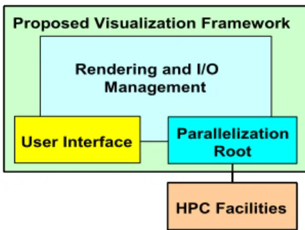
In this paper, we mainly adopted distributed memory architecture for the proposed technique. As shown in Fig. 1, the proposed visualization system consists of central rendering, I/O management, user interface and a data root for communicating with HPC facilities.
Figure 1 Visualization system components
The proposed visualization system is based on the Vi-sualization Tool Kit (VTK) [21], as an application builder for the implementation of several visualization algo-rithms. The core toolkit should be an object oriented cross-platform software package and have an easy inter-face for the classes that perform visualization algorithms, rendering and interaction techniques.
The first challenge is the huge size of the data sets un-der consiun-deration, which cannot be loaded in the main memory of a single workstation. When using distributed memory based visualization, a preprocessing step should be performed to partition the data sets. This step is per-formed by the master computing node in order to facili-tate loading data by the working computing nodes. In this manner, the input to the preprocessing step is several files. Each one contains the datasets of a specific time step. Domain partitioning is considered as one of the most eminent techniques of the out-of-core visualization researches [2].
Each of the input files is parsed and restructured in an OctTree, which has leaves at its end; these leaves represent new smaller files, which will be the input for the computing nodes. Each node in the OctTree consists of a containing cube representing a subset of the main dataset. Starting with the first file that represents the first time step, from time steps, a containing cube is gener-ated to contain all the dataset. The vertices of this cube are inserted into the parent node of the OctTree as an object. Then, the containing cube is decomposed into smaller sub-cubes using three cutting planes perpendicu-lar to the , and axes. Each sub-cube is inserted in the OctTree as a child node for the parent cube. Next, each sub-cube is examined against the stopping condition. If it doesn’t meet the condition, it will be decomposed again into smaller sub-cubes using the same method. These new sub-cubes are also inserted as children for the parent cube in the OctTree. The cubes are to be divided into smaller cubes in a breadth first manner. This process con-tinues until all leafs containing cubes of the OctTree sa-tisfy the stopping condition. A cube is considered sasa-tisfy- satisfy-ing the stoppsatisfy-ing condition, when it represents a segment of the dataset smaller than a predefined threshold. The threshold is defined by the size of the maximum dataset that computing nodes can process independently. Fig. 2 shows a 2D representation of the OctTree for a 2D data set.
Rendering and Time Management Multimodal User Interface Parallelization Root HPC Facility Proposed Visualization System
Rendering and I/O Management Multimodal User Interface Parallelization Root HPC Facilities Proposed Visualization Framework
Rendering and Time Management Multimodal User Interface Parallelization Root HPC Facility Proposed Visualization System
Rendering and I/O Management
User Interface ParallelizationRoot
HPC Facilities Proposed Visualization Framework
Rendering and Time Management Multimodal User Interface Parallelization Root HPC Facility Proposed Visualization System
Rendering and I/O Management Multimodal User Interface Parallelization Root HPC Facilities Proposed Visualization Framework
Rendering and Time Management Multimodal User Interface Parallelization Root HPC Facility Proposed Visualization System
Rendering and I/O Management
User Interface ParallelizationRoot
HPC Facilities Proposed Visualization Framework
Figure 2. Representation of the OctTree for a 2D data grid
IV. PROPOSED VISUALIZATION TECHNIQUES
The proposed technique uses domain partitioning be-tween the computing nodes along with pipelining archi-tecture to distribute computations between the computing nodes and utilize them efficiently. In this manner, the proposed technique combines the use of distributed memory architecture with the shared memory parallelism to improve performance and scalability
A. Path-Line visualization
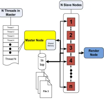
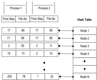
To achieve the best performance and scalability, the proposed technique tries to keep all computing nodes fully utilized all the time. The system architecture for this technique consists of one master node responsible for data preprocessing and handling of tasks, one node work-ing as data storage, one renderwork-ing node and computing nodes as shown in Fig. 3. Message Passing Interface (MPI) is used as the main communication backbone be-tween nodes [22]. After the preprocessing phase, each data file representing a time step is divided into smaller ones. These files are shared between computing nodes. Information about all the computing nodes is stored in a hash table in the master computing node. The key ele-ment of the hash table is the computing node number. The value of each key is an object containing the time step and the file number that is currently loaded in the computing node memory as shown in Fig. 4. For the path-lines to be visualized, a stack of seeding points is constructed on the master computing node and shared between all the other computing nodes.
Figure 3. The proposed Pipeline
Figure 4. Hash table of the computing nodes
The pipeline starts by constructing an OctTree on the master node, while the data set is divided into small ones and transferred to the data storage (as explained before in the preprocessing phase). Each computing node requests a seeding point to process, from the master node, and the master finds the most appropriate one to be sent. To find the mesh cell that contains this seeding point, the corres-ponding computing node searches the OctTree to find the containing sub domain. Next, the computing node applies the Fan Cell Searching algorithm [23] to know which mesh cell contains this seeding point. Then, the compu-ting node interpolates the velocity components and ap-plies the numerical integration method [24] to advance the path-line. The advancement of the path-line is re-turned to the master computing node to be inserted in the queue. Information (like time-step, file number where the seeding point is located, and the cell number that contains the most recent point on the path-line,..) is saved with the seeding point to help the master node in identifying the best computing node for further advancement as shown in Fig. 5. C2 C4 C1 C3 C10 C12 C9 C11 C22 C21 C23 C24 C14 C15 C16 C0 C1 C2 C3 C4 C9 C10 C11 C12 C13 C14 C15 C16 C21 C22 C23 C24
1
2
3
4
n
N Slave Nodes Master Node Render Node Data Storage File 1 File 2 File 3 Thread 1 Thread 2 Thread 3 Thread 4 Shared Memory N Threads in Master Thread N Node 1 Node 2 Node 3 Node 4 Node N 7 1 22 1 10 2 5 2 12 1 File NoFigure 5. Seeding points queue
When computing node requests another seeding point, from the master computing node, the master node identi-fies the file that is already in its memory. Therefore, it sends the most appropriate seeding point to this compu-ting node. This process is performed through searching the queue, for a seeding point, using the time step and the file number. If none is found, the master searches for a seeding point within the same time step only. If there is no seeding point in the same time step, or the file num-ber, the master node sends any seeding point in the next time step to the computing node. This reduces the time needed to load the data file to the computing node’s memory and decreases the number of fetch processes. During the idle time of the master node, it parses the OctTree for each seeding point in the queue to identify its containing sub-cube (file number).
In this fashion, the master computing node starts a sin-gle thread for each computing node. Each thread is re-sponsible for all the communication between the master node and the computing nodes. All these threads share the main memory of the master node, which contains the OctTree. The data storage machine uses memory caching module to reduce the reading time.
B. Computing nodes with multicore processors
The same pipelining architecture is modified to make use of computing nodes with multiple core presences employing OPENMP [25]. In this manner, each compu-ting node will serve with multiple cores running in paral-lel and sharing the same memory. Using multi-core adds some constrains to the technique in order to optimize the usage of the shared memory of the multi-core processor. If we deal with each core as a separate node, each process will load different file in the memory. As the memory capacity of the computing node can load only one data file, the maximum file size in the preprocessing step will be divided by the number of cores per processor. To achieve better utilization for the memory of each compu-ting node, the hash table, that keeps the information about the computing nodes, has to be changed to contain infor-mation about the different cores of each node as shown in Fig. 6. The master node will try to optimize the assign-ment of the seeding points using the information in the
modified hash table. This optimization comes through the assignment of the seeding points located in a single data file to the cores of a single computing node if possible.
Figure 6. Snapshot for the computing nodes hash table for multi-core implementation
C. Stream surface visualization
The implementation of the proposed technique for stream surface visualization is based on the easy integral stream surface algorithm introduced by McLoughlin [23]. This algorithm proposed a special handling for the diver-gence, convergence and rotation.
Figure 7. Convergence and divergence in the flow
The integral surface is constructed from quad primi-tives. The technique is based on two important distances to consider when constructing a new quad: the
dis-tance between neighboring flow line points that corres-pond to the same integration time t and the advance-ment distance. To obtain a smooth and accurate surfaces, the appropriate lengths of and is determined so
that we maintain an appropriate sampling rate of the un-derlying vector field. The sampling rate is guided by the Nyquist Limit, namely, the sampling frequency must be (at least) twice that of the underlying data frequency for accurate reconstruction. Thus we choose an initial :
< ½ .
Divergence and convergence is tested while advancing in the flow field. As soon as any quad reach > 1/2 Seeding Point Queue Point 1 (x,y,z) 1 - -Point2 (x,y,z) 1 17 200 Point3 (x,y,z) 12 17 327 Point4 (x,y,z) 7 4 327 Point M (x,y,z) 17 12 327 Cell No File No Time Step Point Data Node 1 Node 2 Node 3 Node 4 Node N 89 17 22 1 10 2 5 2 89 17 File No
Time Step Hash Table
89 17 89 17 50 2 13 15 78 200 File No Time Step Process 1 Process 2 1/2
d
sepβ
α
S
in+1S
i 1d
isepα
S
i+1β
d
i+1sepS
i+1n+1S
inS
i+1nS
iS
i+2and and we simply divide the
quad. When + < and and
It is handled by terminating the middle flow line. Two quad primitives are merged into a single quad as shown in Fig.7.
V. RESULTS AND DISCUSSION
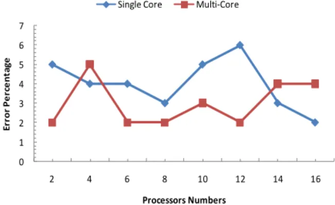
The proposed technique for path-line visualization was tested and evaluated using a 8 GB dataset of the unsteady flow in Driven Cavity [26]. The technique was tested on a cluster of workstations consists of 16 workstations. Each one has a 2.5 GH Pentium Intel processor with dual cores. To confirm the accuracy of the proposed tech-nique, the results of constructing 1000 path-lines using the proposed technique were compared to the results per-formed using VTK (stand alone on a single workstation). The maximum percentage difference introduced with different numbers of computing nodes is shown in Fig. 8 for both of the two modes (the distributed visualization only and the distributed visualization utilizing the multi-cores of each computing node). As shown, the accuracy of the proposed technique is proved, since the difference is within 2- 6%.
The results of constructing a stream surface with 1000 seeding points using the proposed technique were com-pared to the VTK results (stand alone on a single workstation). The maximum percentage difference intro-duced with different numbers of computing nodes is shown in Fig. 9 for both of the two modes.As shown the accuracy of the proposed technique is proved as the dif-ference is within 5- 10%.
Figure 8. Accuracy of the path-lines visualization technique against the results of VTK
Next, the scalability of the proposed techniques was evaluated for both of the two modes in path-lines and stream surface visualization. The processing time for constructing 1000 path-lines and a stream surface was measured as shown in Fig. 10.a and Fig. 10.b. The processing time is drastically decreased as the number of computing nodes increased with better improvement us-ing the second mode (the distributed visualization
utiliz-ing the multi-cores of the compututiliz-ing nodes). The relative speedup for both of the two modes of the proposed tech-niques is shown in Fig. 8.c. This figure indicates that better speedup can be achieved using the multi-core pro-cessors. Both implementations (modes) proved to achieve a good load balancing results as show in Fig. 10.d and Fig. 10.e. All processors achieved good processing utili-zation within an acceptable range between 85- 95% for path-lines and 80-90% for stream surfaces.
Figure 9. Accuracy of the stream surface technique against the results of VTK
VI. CONCLUSION AND FUTURE WORK A distributed path-line and stream surface based visua-lization technique for large 3D time varying vector data is presented and clearly studied. The proposed techniques partition the data sets between the available computing nodes via domain partitioning, and employ a pipelining architecture to decrease the path-lines construction time. The pipeline was modified to fully utilize the computing nodes contains multi-core processors. In this manner, the proposed techniques introduced a hybrid architecture, in which the distributed memory architecture is combined with the shared memory parallelization. The techniques were also used for steam surface visualization. The accu-racy of the proposed techniques was confirmed in com-parison with the results of the VTK (stand alone on a single workstation) with maximum difference of about 6% in path-lines visualization and 10% in stream surface visualization. Then, performance and scalability analyses were conducted for the proposed techniques using data sets with different sizes. The proposed techniques exhi-bited acceptable scalability for different data sizes with better scalability for larger data sets. In addition, the sca-lability improved drastically when utilizing the multi-cores of each computing node. This improvement came close to almost 200% for 16 computing nodes with dual core processors. As a future work, the proposed tech-nique can modified to consider more sophisticated visua-lization methods like flow volumes.
0 2 4 6 8 10 12 2 4 6 8 10 12 14 16 Er ror P e rc e nt ag e Processors Numbers Single Core Multi-Core
0 1 2 3 4 5 6 7 2 4 6 8 10 12 14 16 Er ror P e rc e nt ag e Processors Numbers
a. The processing time (in seconds) for constructing 1000 path-lines
b. The processing time (in seconds) for constructing stream sur-face
c. The speedup for constructing 1000 path-lines d. The load balance for constructing 1000 path-lines
e. The load balance for constructing stream surface Figure 10. Performance and scalability analysis of the proposed technique
REFERENCES
[1] Jinzhu Gao, Chaoli Wang,Liya Li ,Han-Wei Shen “A
parallel multiresolution volume rendering algorithm for large data visualization.” Parallel Computing. 31, 2 Feb. 2005.
[2] Claudio Silva, Jihad El-sana , Peter Lindstrom
Law-rence Livermore “Out-of-Core Algorithms for Scien-tific Visualization and Computer Graphics”. IEEE Vi-sualization, 2002.
[3] S. Bachthaler, M. Strengert,D. Weiskopf,T. Ertl.
"Pa-rallel Texture-Based Vector Field Visualization on Curved Surfaces Using GPU Cluster Computers." Proc. Eurographics PGV Sym, 2006. 75–82.
[4] Ashraf. Hussein, Hesham. El-Shishiny. "A Framework
for Visualization of Large Time-Varying Volume Data for High Performance Computing." Proc. the Center for Advanced Studies on Collaborative research. To-ronto: ACM New York, NY, USA, 2006.
[5] David Lane "A Particle Tracer for Time-Dependent
Flow Fields." Washinton, D.C.: Proc Visualization, 1994. 257 - 264.
[6] Abdelkrim Mebarki, Pierre Alliez, Olivier Devillers.
"Farthest Point Seeding for Efficient Placement of Streamlines." Proc. IEEE Visualization, 2005. 479– 486.
[7] Wijk, Jarke van. "Image Based Flow Visualization." San Antonio, Texas: Proc. Computer graphics and in-0 50 100 150 200 250 300 350 1 2 4 8 16 P roc e ss ing T im e in Se conds Processors Number Single-Core Multi-Core 0 100 200 300 400 500 600 700 800 900 1 2 4 6 8 10 12 14 16 P roc e ss ing T im e in Se conds Processors Number Single-Core Multi-Core 0 0.5 1 1.5 2 2.5 3 3.5 4 4.5 5 1 2 3 4 5 6 7 8 9 10 11 12 13 14 15 16 Spe e du p Processors Number Single-Core Multi-Core 80 82 84 86 88 90 92 94 1 2 3 4 5 6 7 8 9 10 11 12 13 14 15 16 U ti liz at ion P e rc e nt ag e (% ) Processor Id
Single Core Multi-Core
75 80 85 90 95 100 1 2 3 4 5 6 7 8 9 10 11 12 13 14 15 16 U ti liz at ion P e rc e nt ag e (% ) Processor Id Single Core Multi-Core
teractive techniques, 2002. 745 - 754.
[8] Wijk, Jarke van. "Image Based Flow Visualization for
Curved Surfaces." Proc. 14th IEEE Visualization 2003.
[9] Han-Wei Shen, David Kao "A New Line Integral
Convolution Algorithm for Visualizing Time-Varying Flow Fields." IEEE Transactions on Visualization and Computer Graphics, 4, 2 , 1998.
[10]J. Held, J. Bautista,S. Koehl. "Overview, From a Few
Cores to Many:A Tera-scale Computing Research."
In-tel. 2006.
ftp://download.intel.com/research/platform/terascale/te rascale_overview_paper.pdf.
[11]Bjoern Heckel, Gunther Weber, Bernd Hamann,
Ken-neth I. Joy. "Construction of Vector Field Hierar-chies." San Francisco: Proc Visualization, 1999. 19 - 25.
[12]M. Griebel, T. Preusser ,M. Rumpf ,M. A. Schweitzer
,A. Telea. "Flow Field Clustering via Algebraic Multi-grid." Proc Visualization, 2004. 35 - 42.
[13]Gerik Scheuermann, Alyn Rockwood, Heinz Krüger,
Martin Menzel. "Visualizing Nonlinear Vector Field Topology." IEEE Transactions on Visualization and Computer Graphics, 4, 2, 1998.
[14]James L. Helman, Lambertus Hesselink. "Visualizing
Vector Field Topology in Fluid Flows." IEEE Com-puter Graphics and Applications 11. 3, 1991.
[15]David Kenwright, David Lane. "Interactive
Time-Dependent Particle Tracing Using Tetrahedral De-composition." IEEE Transactions on Visualization and Computer Graphics. 1996. 120–129.
[16]Shyh-Kuang Ueng, Christopher Sikorski,Kwan-Liu
Ma. "Out-of-Core Streamline Visualization on Large Unstructured Meshes." IEEE Transactions on Visuali-zation and Computer Graphics. 1997. 370 - 380.
[17]James Ahrens, Kristi Brislawn,Ken Martin,Berk
Ge-veci,C. Charles Law,Michael Papka. "Large-Scale Da-ta Visualization Using Parallel DaDa-ta Streaming." IEEE Computer Graphics and Applications 21, 4 2001, 34 - 41.
[18]Ralph Bruckschen, Falko Kuester, Bernd Hamann,
Kenneth Joy. "Real-time Out-of-Core Visualization of Particle Traces." San Diego, California: Proc IEEE symposium on parallel and large-data visualization and graphics, 2001. 45 - 50.
[19]David Ellsworth, Bryan Green, Patrick Moran.
"Inter-active Terascale Particle Visualization." Washington, DC: Proc Visualization, 2004. 353 - 360.
[20]Hongfeng Yu, Chaoli Wang, Kwan-Liu Ma. "Parallel
Hierarchical Visualization of Large Time-Varying 3D Vector Fields." Proc.ACM/IEEE conference on Super-computing, 2007.
[21]William Schroeder, Kenneth Martin, William
Loren-sen. "The Design and Implementation of an Object-Oriented Toolkit for 3D Graphics and Visualization." San Francisco, California, United States: Proc. 7th conference on Visualization, 1996.
[22]National, University of Chicago-Argonne. MPICH
home page. 2005.
http://www.mcs.anl.gov/research/projects/mpi/mpich2/ .
[23]William Schroeder, Kenneth Martin, William
Loren-sen. Visualization Toolkit: An Object-Oriented Ap-proach to 3D Graphics, 4th Edition. Kitware, 2006.
[24]Philip. Davis, Philip Rabinowitz. “Methods of
Nu-merical Integration”,Second Edition. Dover Publica-tions, 2007.
[25]M. S. Müller, B. R. Supinski,B. M. Chapman.
"Evolv-ing OpenMP in an Age of Extreme Parallelism." Dres-den,Germany: Proc.5th International Workshop on OpenMP, 2009.
[26]S. Albensoeder, H. C. Kuhlmann. "Accurate
Three-Dimensional Lid-Driven Cavity Flow." Journal of Computational Physics 206, 2, 2005, 536 - 558. [27]J. Hultquist. "Constructing stream surfaces in steady
3D vector fields." Proc. Visualization. Bos-ton,Massachusetts: IEEE Computer Society Press, 1992. 171 – 178
[28]Gelder, Allen Van. "Stream surface generation for
flu-id flow solutions on curvilinear grflu-ids." Data Visualiza-tion . Proc. VisSym 01. 2001
[29]Christoph Garth, Xavier Tricoche, Tobias Salzbrunn,
Tom Bobach, Gerik Scheuermann. "Surface Tech-niques for Vortex Visualization." IEEE TCVG Sym-posium on Visualization. 2004
[30]Tobias Schafhitzel, Eduardo Tejada,Daniel
Weiskopf,Thomas Ertl. "Point-based Stream Surfaces and Path Surfaces." Proc. Graphics Interface. 2007. 289 - 296.
[31]Christoph Garth, Han Krishnan,Xavier Tricoche,Tom
Tricoche,Kenneth I. Joy. "Generation of Accurate Integral Surfaces in Time-Dependent Vector Fields." IEEE Transactions on Visualization and Computer Graphics. 14 , 6, 2008, 1404-1411.
[32]Tony McLoughlin, Robert S. Laramee, and Eugene
Zhang. "Easy integral surfaces: a fast, quad-based stream and path surface algorithm." Computer Graph-ics International. New York, 2009. 73-82 .