Consensus Network Inference of Microarray Gene
Expression Data
Suhaib Mohammed University of Exeter
Doctor of Philosophy in Biological Sciences In July 2016
This thesis is available for Library use on the understanding that it is copyright material and that no quotation from the thesis may be published without proper
acknowledgement.
I certify that all material in this thesis which is not my own work has been identified and that no material has previously been submitted and approved for the award of a degree by this or
any other University.
“Everything is theoretically impossible, until it is done”
3
Abstract
Genetic and protein interactions are essential to regulate cellular machinery. Their identification has become an important aim of systems biology research. In recent years, a variety of computational network inference algorithms have been employed to reconstruct gene regulatory networks from post-genomic data. However, precisely predicting these regulatory networks remains a challenge.
We began our study by assessing the ability of various network inference algorithms to accurately predict gene regulatory interactions using benchmark simulated datasets. It was observed from our analysis that different algorithms have strengths and weaknesses when identifying regulatory networks, with a gene-pair interaction (edge) predicted by one algorithm not always necessarily consistent with the other. An edge not predicted by most inference algorithms may be an important one, and should not be missed. The naïve consensus (intersection) method is perhaps the most conservative approach and can be used to address this concern by extracting the edges consistently predicted across all inference algorithms; however, it lacks credibility as it does not provide a quantifiable measure for edge weights. Existing quantitative consensus approaches, such as the inverse-variance weighted method (IVWM) and the Borda count election method (BCEM), have been previously implemented to derive consensus networks from diverse datasets. However, the former method was biased towards finding local solutions in the whole network, and the latter considered species diversity to build the consensus network.
In this thesis we proposed a novel consensus approach, in which we used Fishers Combined Probability Test (FCPT) to combine the statistical significance values assigned to each network edge by a number of different networking algorithms to produce a consensus network. We tested our method by applying it to a variety of in silico benchmark expression
datasets of different dimensions and evaluated its performance against individual inference methods, Bayesian models and also existing qualitative and quantitative consensus techniques. We also applied our approach to real experimental data from the yeast (S. cerevisiae) network as this network has been comprehensively elucidated previously. Our results demonstrated that the FCPT-based consensus method outperforms single algorithms in terms of robustness and accuracy. In developing the consensus approach, we also proposed a scoring technique that quantifies biologically meaningful hierarchical modular networks.
5
Acknowledgements
This research project would not have been completed without the following people. First and foremost, I would like to thank my primary supervisor, Dr. Zheng Rong Yang, for his guidance, valuable support and critical feedback throughout this project. I also extend my deepest gratitude to my secondary supervisor, Dr. Ozgur E. Akman, for his vital suggestions, and comments in and out of lab meetings. Without their support, it would have been difficult to accomplish this research. Furthermore, I would like to thank my external examiner, Dr. Guido Sanguinetti, and internal examiner, Dr. Ed Keedwell for their feedback and suggestions, which improved the quality of this thesis.
I am very grateful to my friends and lab colleagues, Varun Kothamachu, Abdul Latif, Ben Wareham, Jason Bullock for providing suggestions and support during our period of time spent in Exeter. I was fortunate to come across Erratics Cricket Club, who helped enable me to meet many wonderful people, motivating throughout the duration of the project.
I would personally like to thank my wife, Umme Salma, for her constant moral support and encouragement, especially during the most arduous periods. Despite being pregnant during my final research and thesis write up stage, she motivated me and provided me space to concentrate. I also owe a big thank you to my mother for her unconditional support and constant encouragement by telephone despite her residence in the Asian subcontinent.
Last but not least, I thank my newborn daughter, Safaa. She has given me reason to smile during the most stressful times of my thesis write-up. Finally, I extend my gratitude and thankfulness to the University of Exeter Studentship for supporting me financially during the course of my research.
Table of Contents
Abstract ... 3! Acknowledgements ... 5! Table of Contents ... 6! List of Figures ... 9! List of Tables ... 14! Authors Declaration ... 16 1. Introduction ... 17! 1.1! General Introduction ... 18!1.2! Modularity in biological networks ... 21!
1.2.1!Modularity ... 22!
1.2.2!Network Robustness ... 22!
1.3! Network graphs ... 23!
1.3.1!Directed and undirected graphs ... 23!
1.3.2!Weighted graphs ... 24!
1.4! Microarray datasets ... 24!
1.4.1!Single channel microarray experiments ... 25!
1.4.2!Two channel microarray experiments ... 26!
1.4.3!Steady-state microarray experiments ... 26!
1.4.4!Time series microarray experiments ... 27!
1.5! Reconstruction of gene networks ... 27!
1.6! Motivation behind the study ... 29!
1.6.1!Fishers combined probability test ... 32!
1.7! Aims and Objectives ... 33!
1.8! Thesis Overview ... 34
2.! Background and literature review ... 36!
2.1! Modelling gene regulatory networks ... 37!
2.1.1!Information theory models ... 38!
2.1.2!Bayesian network models ... 47!
2.1.3!Differential equation models ... 51!
2.1.4!Other approaches ... 52!
2.2! Consensus methods ... 53!
2.3! Qualitative approaches ... 53!
7
2.3.2!Union method ... 55!
2.4! Quantitative approaches ... 57!
2.4.1!Combining p-values ... 58!
2.4.2!Combining ranks ... 62!
2.4.3!Directly merging raw data ... 64!
2.5! Discussion and Conclusion ... 64
3.! A consensus approach to predict regulatory interactions ... 67!
3.1! Introduction ... 68!
3.2! Methods and Material ... 72!
3.2.1!Benchmark algorithms ... 72!
3.2.2!Generating a consensus network ... 72!
3.2.3!False Discovery Rate control ... 73!
3.2.4!Network Validation ... 73!
3.2.5!Scoring Method ... 77!
3.2.6!Estimation of significance values ... 80!
3.3! Results ... 91!
3.3.1!DREAM4 size 10 ... 98!
3.3.2!DREAM4 size 100 ... 99!
3.3.3!Consensus edges - overlap statistics ... 100!
3.3.4!Noise and Robustness ... 104!
3.3.5!Combining inference methods ... 106!
3.3.6!Comparison with existing consensus methods ... 108!
3.4! Discussion ... 123!
3.5! Conclusions ... 126
4.! Comparative analysis of network algorithms to address modularity ... 128!
4.1! Introduction ... 129!
4.2! Materials and Methods ... 132!
4.2.1!Datasets ... 132!
4.2.2!Performance measurements ... 133!
4.2.3!Results & Discussion ... 142!
4.2.4!Conclusions ... 167
5.! Application of consensus approach to study yeast network ... 169
5.1! Yeast network ... 170!
5.3! Network Validation ... 174!
5.4! Results and Discussion ... 176!
5.4.1!Hierarchical Modularity ... 185!
5.5! Conclusions ... 198
6.! Conclusion and future work ... 200!
6.1! Summary ... 200!
6.2! Limitations of the study ... 205!
6.3! Future work ... 206
7.! Appendix A ... 208!
8.! Appendix B ... 217!
9
List of Figures
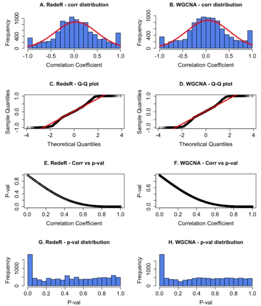
Figure 1.1: The above schematic depicts the different levels at which biological networks can be described ... 19 Figure 1.2. Sample directed (A) and undirected (B) networks with 6 nodes (A, B, C, D, E and F) representing genes (or proteins). ... 23 Figure 1.3. A sample weighted (A) and unweighted network (B). The network attributes are the same as in Figure 1.2. ... 24 Figure 1.4. Schematic illustrating the flow process of a single channel microarray (left panel) and a two-channel microarray (right panel). This figure was adapted from (Serra 2011). ... 25 Figure 1.5. The flow process for gene regulatory network using reverse engineering approaches. ... 28 Figure 1.6: A). Common approach used to build a consensus network from multiple microarray experiments using a single inference method. ... 31 Figure 2.1: Flow chart for choosing a suitable network inference algorithm depending on the type of gene expression data used. ... 38 Figure 2.2: Hierarchical modular network structure from RedeR. ... 40 Figure 2.3: A sample intersection consensus network D and corresponding adjacency matrix ... 55 Figure 2.4: A sample union consensus network D and corresponding adjacency matrix ... 56 Figure 2.5: A sample quantitative consensus network D derived from the networks A, B and C ... 57 Figure 2.6: An example 4-gene true network (A) used for building a community consensus network. ... 63 Figure 3.1: Flow process of the validation framework using benchmarked in silico datasets 74 Figure 3.2: The distribution of frequency statistics calculated using a parametric approach. 81 Figure 3.3: Workflow illustrating the process of calculating p-values from an example gene expression matrix ... 84 Figure 3.4: Illustrates a new permutation-based algorithm to estimate significance values ... 85 Figure 3.5: A: Histogram showing the distribution of correlation coefficients calculated by WGCNA ... 86 Figure 3.6: Flow process for estimating p-values using parametric and non-parametric approaches ... 87
Figure 3.7: Shows the distribution of p-values estimated using two different approaches ... 88
Figure 3.8: The distribution of frequency statistics for MI inference algorithms calculated using the non-parametric permutations ... 90
Figure 3.9: Shows gold standard true in silico network of size 100 and size 500 ... 92
Figure 3.10: Similarity between different network inference algorithms ... 93
Figure 3.11: ROC curves and corresponding AUROC estimates for individual network ... 96
Figure 3.12: Comparing the performances of consensus network by FCPT against individual network inference ... 97
Figure 3.13: Performance scores of different network inference approaches using benchmarked DREAM4 challenge in silico datasets of size 10 ... 99
Figure 3.14: Compares performance scores of different network inference approaches using benchmarked DREAM4 challenge in silico datasets of size 100 ... 100
Figure 3.15: Overlap ratio of edges predicted by the consensus network method (FCPT) and individual inference methods ... 101
Figure 3.16: Number of unique edges predicted by the consensus (FCPT) network that are not common ... 102
Figure 3.17: Sensitivity measures for edges predicted by consensus (FCPT) and individual inference methods ... 104
Figure 3.18: Comparative performance scores of individual and integrated network inference approaches ... 107
Figure 3.19: Venn diagrams showing the number of common predicted edges across different network inference algorithms ... 109
Figure 3.20: Sensitivity and specificity values obtained with qualitative consensus methods (intersection and union) ... 111
Figure 3.21: Gold standard (true) network (left plot) and predicted consensus network by FCPT at significance threshold q<0.05 (right plot) obtained from a benchmark in silico expression dataset of size 100 ... 112
Figure 3.22: Gold standard (true) network (left plot) and predicted consensus network by FCPT at significance threshold q<0.05 (right plot) obtained from a benchmark in silico expression dataset of size 500 ... 113
Figure 3.23: ROC curves and corresponding AUROC values for existing quantitative consensus approaches using benchmarked in silico datasets of size (nodes) 100 and size 500 ... 115
Figure 3.24: Performance scores of equantitative consensus methods using benchmarked DREAM4 challenge in silico datasets of size 10 ... 116
11
Figure 3.25: Performance scores of quantitative consensus methods using benchmark DREAM4 challenge in silico datasets of size 100 ... 118 Figure 3.26: AUROC scores obtained by combining different inference methods using in silco datasets ... 122 Figure 4.1: Pyramid structure of a cell’s complexity. Information quantity and level of complexity ... 129 Figure 4.2:The flow process of GO enrichment analysis for each identified module. ... 139 Figure 4.3: The workflow for deriving module and model scores. ... 142 Figure 4.4: Hierarchical and modular network consisting of 8 modules with size 100 and size 500 gene expression data. ... 143 Figure 4.5: Average silhouette width, Dunn index and Separation index calculated for different numbers of cluster modules ... 145 Figure 4.6: Number of enriched GO terms found for different number of modules generated from size 100 and size 500 in silico datasets ... 147 Figure 4.7: Percentage of annotated GO terms found for different numbers of modules generated from size 100 and size 500 in silico datasets ... 148 Figure 4.8: Gene ontology enrichment analysis for 4 cluster modules that are significantly enriched for biological processes with size 100 data ... 152 Figure 4.9: Gene ontology enrichment analysis for 8 cluster modules that are significantly enriched for biological processes with size 100 data. ... 153 Figure 4.10: Gene ontology enrichment analysis for 12 cluster modules that are significantly enriched for biological processes with size 100 data. ... 154 Figure 4.11: Gene ontology enrichment analysis for 16 cluster modules that are significantly enriched for biological processes with size 100 data. ... 155 Figure 4.12: : Gene ontology enrichment analysis for 4 cluster modules that are significantly enriched for biological processes with size 500 data. ... 156 Figure 4.13: Gene ontology enrichment analysis for 8 cluster modules that are significantly enriched for biological processes with size 500 data. ... 157 Figure 4.14: Gene ontology enrichment analysis for 12 cluster modules that are significantly enriched for biological processes with size 500 data. ... 158 Figure 4.15: Gene ontology enrichment analysis for 16 cluster modules that are significantly enriched for biological processes with size 500 data. ... 159 Figure 4.16: Module and model scores for the top enriched GO terms for different numbers of modules with size 100 data. ... 162
Figure 4.17: Module and model score for top enriched GO term found for different number of modules with size 500 data. ... 164 Figure 4.18: Model scores obtained using different network algorithms for various numbers of modules with size 100 (left) and size 500 (right) data. ... 166 Figure 5.1: Schematic depicting the gene selection process by differential gene expression analysis, contrasting consecutive comparison against non-consecutive comparison. ... 171 Figure 5.2: Statistically significant DEGs (q<0.01) changing across consecutive and non-consecutive time points. ... 173 Figure 5.3: Network validation workflow for real gene expression data. ... 175 Figure 5.4: Correlation coefficients (A and B) and mutual information values (C, D and E) generated from all gene pair interactions (edges) plotted against corresponding p-values for different network algorithms. ... 177 Figure 5.5: A-E: significance p-value distribution plots obtained from the individual network algorithms. F: the corresponding distribution of Fisher’s combined test statistic. ... 178 Figure 5.6: ROC curves showing the relationship between sensitivity and specificity for individual network inference methods (A) and consensus approaches (B) using a real gene expression dataset. ... 179 Figure 5.7: Using AUROC measures to compare the performance of the individual and consensus network inference algorithms ... 180 Figure 5.8: AUROC scores obtained using real gene expression data from S.cerevisiae with the top performing inference algorithm ... 181 Figure 5.9: A) Venn diagram comparing the statistically significant interactions (p<0.05) obtained using five different network inference algorithms. ... 182 Figure 5.10: Gold standard and predicted consensus networks. ... 183 Figure 5.11: Hierarchical and modular networks consisting of 8 modules obtained with real gene expression data. ... 186 Figure 5.12: Internal validation indices. Average silhouette width, Dunn index and Separation index calculated for different numbers of cluster modules generated from each of the network algorithms using realgene expression data. ... 186 Figure 5.13: A) Number of enriched GO terms found for different numbers of modules generated from real gene expression data at various p-value cutoffs. ... 188 Figure 5.14: GO enrichment analysis for 4 cluster modules that are significantly enriched for BPs, using real gene expression data. ... 191 Figure 5.15: GO enrichment analysis for 8 cluster modules that are significantly enriched for BPs, using real gene expression data. ... 192
13
Figure 5.16: GO enrichment analysis for 12 cluster modules that are significantly enriched for BPs, using real gene expression data. ... 193 Figure 5.17: GO enrichment analysis for 16 cluster modules that are significantly enriched for BPs, using real gene expression data. ... 194 Figure 5.18: Modular and model scores for the top enriched GO terms for different numbers of modules with real gene expresion data. ... 195 Figure 5.19: Model scores obtained using different network algorithms for a various numbers of modules with real gene expression data. ... 196 Figure 6.1: Sample network showing high degree nodes called hubs highlighted in blue.The yellow nodes signify genes. ... 206 Figure A.1: ROC curves and corresponding AUROC values for different network inference approaches using a benchmarked in silico dataset of size (nodes) 100 ... 209 Figure A.2: Comparative average performance scores of different network inference approaches using benchmarked in silico datasets generated from SynTReN of size 100 and size 500 ... 210 Figure A.3: Performance scores of different network inference approaches using benchmarked DREAM4 challenge in silico datasets of size 10. ... 212 Figure A.4: Performance scores of different network inference approaches using benchmarked DREAM4 challenge in silico datasets of size 100. ... 213
List of Tables
Table 3.1: Descriptions of the benchmark in silico networks and corresponding datasets used in the validation framework ... 75! Table 3.2: Summary of the confusion matrix used to classifiy edge predictions. ... 78! Table 3.3: AUROC scores obtained by applying different inference methods to in silico datasets of size 100 and size 500 ... 105! Table 3.4: Average processing times (in seconds) for different consensus methods ... 119! Table 3.5: AUROC scores for different consensus methods obtained from SynTReN datasets ... 120! Table 4.1: Benchmark network inference algorithms and corresponding data types they support. ... 132! Table 4.2: Functional top ranked modules from different network algorithms that show statistically significant (p<0.05) association to biological process in GO enrichment analysis for size 100 data. ... 163! Table 4.3: Functional top ranked modules from different network algorithms that show statistically significant (p<0.05) association to biological process in GO enrichment analysis for size 500 data. ... 165! Table 5.1: Performance statistics for individual network inference methods ... 185! Table 5.2: Functional top ranked modules from different network algorithms that show statistically significant (p<0.05) association to biological process in GO enrichment analysis from real gene expression data. ... 197! Table 6.1: The gain in average performance by consensus network in terms of fold changes from different sized datasets. ... 203! Table A.1: Consensus-predicted unique edge-lists those are not common across individual network inference algorithms using real gene expression data from S.cerevisiae. ... 214! Table B.1: Functional modules predicted from RedeR for different cluster module sizes that show statistically significant (p<0.05) association with biological process (BP) in GO enrichment analysis for size 100 data. ... 217! Table B.2: Functional modules predicted from WGCNA for different cluster module sizes that show statistically significant (p<0.05) association with biological process (BP) in GO enrichment analysis for size 100 data. ... 218! Table B.3: Functional modules predicted from SIMoNE for different cluster module sizes that show statistically significant (p<0.05) association with biological process (BP) in GO enrichment analysis for size 100 data. ... 219!
15
Table B.4: Functional modules predicted from RedeR for different cluster module sizes that show statistically significant (p<0.05) association with biological process (BP) in GO enrichment analysis for size 500 data. ... 219! Table B.5: Functional modules predicted from WGCNA for different cluster module sizes that show statistically significant (p<0.05) association with biological process (BP) in GO enrichment analysis for size 500 data. ... 221! Table B.6: Functional modules predicted from SIMoNE for different cluster module sizes that show statistically significant (p<0.05) association with biological process (BP) in GO enrichment analysis for size 500 data. ... 222! Table B.7: Functional modules predicted from RedeR for different cluster module sizes that show statistically significant (p<0.05) association with biological process (BP) in GO enrichment analysis with real gene expresson data. ... 223! Table B.8: Functional modules predicted from WGCNA for different cluster module sizes that show statistically significant (p<0.05) association to biological process (BP) in GO enrichment analysis with real gene expresson data. ... 224! Table B.9: Functional modules predicted from SIMoNE for different cluster module sizes that show statistically significant (p<0.05) association to biological process (BP) in GO enrichment analysis with real gene expresson data. ... 226!
Authors Declaration
This work includes material from published papers from conference proceedings, which contribute to the content of the thesis. These published papers, are contributions to the thesis content during the period of the author’s study at the University of Exeter. All other material which is not my own, has been identified and referenced accordingly. I hereby declare that I am the sole author of this thesis.
Published papers from the conference proceedings
• Mohammed, S., Akman, O. E., & Yang, Z. R. (2014). A consensus approach to
predict regulatory interactions. In 2014 7th International Conference on Biomedical Engineering and Informatics (pp. 769–775). Dalian, China: IEEE. doi:10.1109/BMEI.2014.7002876 (Included in Chapter 3)
• Mohammed, S. (2013). Comparative analysis of network algorithms to address
modularity with gene expression temporal data. In ACM Conference on Bioinformatics, Computational Biology and Biomedical Informatics Proceedings (Vol. 978–1–4503, pp. 876–882). Washington, USA: ACM Digital Library. doi:10.1145/2506583.2506698 - (Included in Chapter 4 and Chapter 5)
17
Chapter 1
Introduction
Abstract
This chapter provides a general introduction to the subject of modelling biological networks; the discussion of different biological networks applied in systems biology research, the purpose of biological network inference and the implication of transcriptional networks. Elementary concepts and definitions of network properties, and biological data used for network reconstruction are also discussed. Finally, the motivation for this study, including its novelty aspects are discussed.
1.1
General Introduction
A cell is a functional unit of life that serves as a building block for all living organisms. The large quantity of coded information stored in the DNA of a cell’s genes coordinates complex biological processes. Complexity is the hallmark of cellular systems. The regulatory interaction between the genes and its products (proteins) orchestrates this complexity. As a result the biological information is transferred via several pathways (e.g. signalling, regulatory and metabolic), which form complex regulatory networks between biological entities such as DNA, RNA, proteins and metabolites. Therefore, a key challenge is to understand the structure and relationship between genes that coordinate multiple functions of a living cell within a dynamically changing environment (Bennett et al. 2008).
The post-genomic era is invariably shifting from annotating individual genes and proteins to understanding complex interactions between biological entities inside the cell, to investigating regulatory signalling and metabolic pathways when exposed to external perturbations (Cassman et al. 2007). In order to understand this complexity, contemporary scientists depend on the “reductionist” approach - employing mathematical modeling tools and techniques to understand biological complexity at molecular levels. This approach has been pursued in the past two decades to characterize and identify regulatory interactions, starting from a gene or protein of interest, and trying to uncover its involvement in the same or different pathways. By integrating knowledge of biological data using hypothesis-driven research and employing mathematical modeling tools, we can explore the functions of genes and proteins, and gain insights into the mechanisms underlying biological activity.
Systems biology aims to understand the physiology of living systems on a whole, rather than in parts (Ma’ayan 2011). Networks or graphs provide mathematical abstraction when representing a broad variety of complex systems, such as the internet, social interactions, and
19
biological and ecological systems (Albert R 2002; Barabási & Oltvai 2004). To some extent, biology researchers embrace the network description as it compactly depicts the control system of the cell, which represents the expression of all genes in tight coordination (Haiyuan Yu, Nicholas M Luscombe 2003) as shown in Figure 1.1.
Figure 1.1: The above schematic depicts the different levels at which biological networks can be described. Gene A shows the autocrine effect, in which it regulates its own gene transcription; the product of gene A also influences the transcription of gene B, with gene B having an effect on the transcription of gene C.
Biological networks are composed of nodes and edges. The former represent biological entities, whilst the latter illustrates the regulatory relationship between the entities. High throughput technology data - like transcriptomics, proteomics and metabolomics - have enabled researchers to consider genome-wide approaches to understand and analyze biological entities on a global level. Cellular components do not work alone, but instead, interact with each other within a highly complex structure. The schematics in Figure 1.1 depict the central dogma of molecular biology, whereby genetic material (DNA) is
transcribed into RNA molecules, and then translated into proteins. The proteins are the end products and carry out a vast array of functions, including acting as transcription factors (TFs) that promote (or repress) transcription, catalyzing metabolic reactions and transporting molecules at different locations (Desvergne et al. 2006).
In order to uncover the complex behavior of the biological system, it is imperative to define biological entities and their interactions within a model (Hecker et al. 2009). Therefore, representing the complex interactions between genes and proteins using networks enables us to visualize and unfold the mechanism of the underlying biological process. Biological networks can be reconstructed using various network inference algorithms (Hecker et al. 2009; Markowetz & Spang 2007). Once an algorithm is chosen, optimized parameters are required to fit the data used in the reconstruction process.
Contemporary experimental technologies provide heterogeneous high-throughput data that enables us to measure biological networks and their components at various levels. These include mRNA transcripts measurements, protein abundance and metabolite quantification. The summary of such networks at multiple levels is described below.
• Transcriptional networks describe the transcriptional regulation of genes through
proteins called transcription factors (TFs). Nodes indicate genes (or proteins), and edges denote physical or regulatory interactions. A directed edge between a source and target gene, represents a transcriptional activator (positive regulation) or inhibitor (negative regulation) that controls the production of an RNA or protein molecule. Such networks - also referred to as gene regulatory networks (GRNs) - encapsulate direct and indirect regulatory relationships between genes. For example, in Figure 1.1, gene A shows the autocrine effect as it regulates its own gene transcription through synthesised protein. Gene A also influences the transcription of gene B, which has an effect on the transcription of gene C. To study the physical interaction between a TF
21
and the promoter of a target gene, the Chromatin immunoprecipitation (ChIP) experiment is commonly performed to determine whether a particular protein (TF) binds to the specified DNA sequence (Promoter) (Carey et al. 2009).
• Protein networks describe the physical interactions between their components, like
binding and complex formation. In such graphs, also referred to as protein-protein interaction networks, a node indicates a protein, whilst an edge represents the interaction between two nodes (molecules). A yeast-two-hybrid screen is used to experimentally verify the physical interactions between pairs of protein molecules (Miller & Stagljar 2004).
• Metabolic networks describe a set of metabolites and the corresponding set of
chemical reactions, which are associated with the metabolites. In such networks, metabolites are assigned as nodes and the edges represent the biochemical reaction catalysed by an enzyme (protein) between a substrate-product pair (Hatzimanikatis et al. 2004). Mass-Spectrometry (MS) techniques are widely employed to identify potential metabolites (Weckwerth 2003).
1.2
Modularity in biological networks
Uncovering the topology and dynamics of biological networks can provide useful insights into how a cell responds to a specific external perturbation, when executing complex biological processes. Outlined below are some of the notable characteristics of biological networks that enable us to understand their function.
1.2.1 Modularity
One prominent characteristic of biological networks are their embedded modular structure (Barabási & Oltvai 2004). A modular system is composed of subsystems which each perform specific functions autonomously. A biological network - which is sparsely interconnected - exhibits such modularity, which in turn facilitates specific biological functions. Specifically, densely populated sets of nodes (genes or proteins) - that are linked functionally or physically and which regulate a signaling or metabolic pathway - are called hubs (Blais & Dynlacht 2005). These densely colonized hubs display a modular structure, sharing common biological functions and showing similar expression patterns in response to external perturbations to the subnetwork. For example, those groups of genes that are co-regulated with respect to time govern the different stages of the cell cycle (Simon et al. 2001).
Hierarchical modular architecture is an extension of modularity that delineates how biologically related functional modules are organised within the network. Many biological networks - ranging over metabolic, protein and genetic interactions - show signatures of hierarchical topology, in which functional modules do not independently coexist, but combine in a hierarchical fashion for governing entities of biological process (Ravasz & Barabási 2003; Yu & Gerstein 2006).
1.2.2 Network Robustness
Biological systems are robust, responding to various external and internal perturbations, whilst still being able to perform their biological functions (Barabási & Oltvai 2004). In a topological sense, environmental perturbations and other effects cause mutations of genes under which the networks continuously evolve. To cope with the effect of these perturbations, biological networks adapt their robustness in order to attain phenotypic stability. The mechanisms through which the networks are rewired to resist these changes and
23
restore stability are redundancy (i.e. duplication of the genome), positive and negative feedback control, and degeneracy (i.e. different biological entities of the network performing the same function in order to yield the same effect or output) (Barabási & Oltvai 2004; Blais & Dynlacht 2005). It has been argued that modules facilitate this adaptation of robustness, as they are able to maintain a cellular function despite the malfunctioning of genes under specific external perturbations. For example, the mutation of many single genes by deletion in Saccharomyces cerevisiae has had an insignificant effect on the organism’s growth rate (Breslow et al. 2008).
1.3
Network graphs
A network is represented by a graph in mathematical terminology. A graph G with no multiple edges and loops is a pair of sets (V(G), E(G)) where V(G) represents a set of nodes or vertices, and E(G) represents a set of edges, each of which links two nodes.
1.3.1 Directed and undirected graphs
Figure 1.2. Sample directed (A) and undirected (B) networks with 6 nodes (A, B, C, D, E and F) representing genes (or proteins). Edges represent the directional interaction between two genes/proteins and their functional relationship.
A directed graph is one in which edges have specific directions or arrows, whereas in an undirected graph, edges have no directions. A directed edge indicates a causal relationship between two nodes if an edge exists. A sample directed and undirected graph is shown in Figure 1.2(A-B), where each node corresponds to a gene and edges corresponds to the relationship between two genes.
1.3.2 Weighted graphs
Figure 1.3. A sample weighted (A) and unweighted network (B). The network attributes are the same as in Figure 1.2.
A weighted graph is one where each edge has an associated weight, reflecting the strength of the connection between the two nodes. The weights can be either positive or negative numbers, indicating whether the edge represents activation or inhibition respectively. By contrast, an unweighted graph has no weights associated with its edges. A simple weighted and unweighted graph is shown in Figure 1.3(A-B).
1.4
Microarray datasets
The generation of high throughput data has become increasingly prevalent over the last decade. Microarray technology, in particular, has enabled expression levels to be measured
25
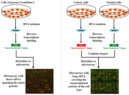
for large number of genes. The underlying principle across all microarray experiments is the same. A microarray consists of a silicon chip or glass slide that carries a large number of immobilized short single-stranded DNA sequences (ssDNAs) - more commonly known as probes. Hybridization experiments are carried out with labeled mRNAs, which attach to the probes with a reverse complementary sequence. Gene expression levels are quantified by a counting the number of labeled mRNAs bound to each probe using a scanning device. The most common microarray platforms are the single channel experiment and the two channel experiment (Ness 2006), both shown in Figure 1.4.
Figure 1.4. Schematic illustrating the flow process of a single channel microarray (left panel) and a two-channel microarray (right panel). This figure was adapted from (Serra 2011).
1.4.1 Single channel microarray experiments
A single channel experiment is also known as an oligonucleotide microarray. This means that in one experiment, only one target sample is analysed. In this platform, genes are represented
by a set of short ssDNA carrying probes - oligonucleotides (i.e. 25 mer probes). Target mRNAs are labelled fluorescently and probe-target hybridization is quantified by the detection of fluorescence signals using a scanning device (Figure 1.4-left panel). These arrays provide raw measures of expression for each individual gene (i.e. absolute expression levels). Popular single channel arrays are Affymetrix Gene Chips. A key advantage of oligonucleotide microarrays is their high specificity. For example, during the design process of the oligonucleotide sequence for a particular gene, each gene of the target gene sequence perfectly complements another; concomitantly, its partner sequence is deliberately designed to have a single base mismatch in its centre. This minimises the effects of non-specific binding.
1.4.2 Two channel microarray experiments
Two channel microarrays are also known as cDNA (complementary DNA) microarrays. These use single-stranded cDNA sequences as probes. This platform allows the sampling of mRNA from two different conditions within the same experiment, labelled with two distinct types of dyes – Cy3 (green) and Cy5 (red). Essentially, one of the labelled dyes is used as a control and the other as the experimental condition of interest (for example – disease, time point, etc.), as shown in the right panel of Figure 1.4. Target mRNAs are labelled with fluorescent dyes and expression levels are quantified by two scanning devices that detect Cy3 and Cy5 signals respectively. These arrays measure the relative difference in gene expression levels.
1.4.3 Steady-state microarray experiments
Steady-state microarray experiments sample the expression of all mRNAs at a single time point following the perturbation of a target gene (Wang et al. 2013). Here, perturbation refers
27
to the genetic manipulation of the genome (knock-out, knockdown or over-expression). Steady-state data does not capture the dynamics of the biological system, but it provides information as to how the expression levels of all the genes are influenced by that of a particular gene.
1.4.4 Time series microarray experiments
Time series microarray data is used to explore the dynamics of biological systems when exposed to environmental perturbations (e.g. chemical stress, heat shock, and drug treatments) (Wang et al. 2013). Here, all mRNAs are sampled at consecutive time points, from the time the external signal is introduced into the system. Time series data captures the dynamics of the experiment, and it allows delineating directional interactions between genes to understand the cause and effect relationship. The profile obtained by plotting gene expression against sampling time then quantifies the expression dynamics (Androulakis et al. 2007).
1.5 Reconstruction of gene networks
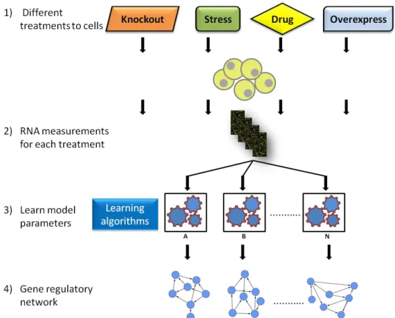
The reconstruction of GRNs based on gene expression data is known as network inference or reverse engineering. GRN reconstruction primarily uses RNA expression levels measured by microarray experiments across different experimental conditions (Figure 1.5). Typically two types of data are used: steady state and time series (see 1.4.3 and 1.4.4 above). GRN reconstruction has two main aims: locally, to determine how one gene's activity affects another gene’s activity; and globally, to determine how genes collectively respond to a perturbation. The inferred interactions can, for example, be TF-gene interactions or gene-gene interactions (Hecker et al. 2009).
In the past few years, several network inference algorithms have been developed. However, identifying GRNs in an accurate and robust manner still remains a challenge (Penfold & Wild 2011). These algorithms are broadly graded into two classes: 1) algorithms that attempt to uncover “physical interactions” - these aim to identify protein-gene interactions (i.e. TF binding on the cis-regulatory region of a target promoter genomic DNA sequence); and 2) algorithms that attempt to uncover “influence interactions” by identifying the regulatory relationship between genes based on expression dynamics (i.e. gene-gene interactions). Here, both classes are referred to collectively as “regulatory interactions”.
Figure 1.5. The flow process for gene regulatory network using reverse engineering approaches. A and B represents different network inference algorithms and N indicates the number of algorithms used.
29 1.6 Motivation behind the study
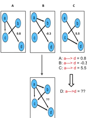
Recent evidences have suggested that when different inference methods are applied to the same microarray dataset, inconsistent predictions occur (De Smet & Marchal, 2010; Maetschke, Madhamshettiwar, Davis, & Ragan, 2014; Marbach et al., 2010) which is not surprising - as depicted in Figure 1.5, a gene pair interaction (edge) predicted from one network inference algorithm may not always be necessarily predicted by the other. One way of dealing with this discrepancy in predictions is to combine the results obtained from different inference algorithms, thereby forming an ensemble that delivers more robust predictions. Furthermore, this is an intuitive step for better coverage of gene interactions, consequently, it increases sensitivity. There are two ways to build up such an ensemble: conservative (qualitative) or profitable (quantitative). The conservative method provides a simple way of combining predictions to deliver a consensus output, based on the consistency of patterns or topology, without much importance given to numerical values. That is, the common predicted edge interactions by network algorithms used. Despite their simplicity, a major drawback of conservative methods is that they fail to provide quantifiable measures and so important interactions can be missed. The profitable method combines the predictions obtained from independent studies using statistical techniques (Borenstein & Rothstein 2007). This meta-analysis approach has been successfully applied in diverse areas - from genomic research for detecting differentially expressed genes by combining multiple gene expression profiles (Chang et al. 2013) to medical research for integrating the results of independent clinical trial studies (DerSimonian & Laird 1986). Therefore, the success of meta-analysis approaches in other disciplines motivated us to investigate its potential to produce more robust, and accurate networks that solves network inference problem.
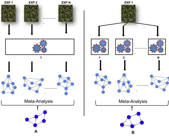
In recent years, there have been several studies exploring meta-analysis techniques for combining results in the field of network inference (Tseng et al. 2012; Steele & Tucker
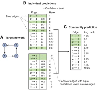
2008). However, most studies focused on combining predictions from multiple expression datasets using a single inference method, as shown in Figure 1.6A. For instance, Wang et al (Wang et al. 2006) combined networks from multiple time series microarray experiments performed in different conditions to construct a GRN using linear programming. Similarly, Niida et al (Niida et al. 2010) built a cancer transcriptional network using a conservative meta-analysis approach. More specifically, a meta-network was deduced after superimposing consistent networks that were predicted, after EEM based algorithm was applied to each of the several cancer microarray experiments. In another study, Steele et al (Steele & Tucker 2008) applied statistical meta-analysis approach to construct a consensus Bayesian network by combining edge interactions using results obtained from single Bayesian inference algorithm using multiple microarray datasets. They implemented inverse-variance weighted method (IVWM) (DerSimonian & Laird 1986) as a meta-analysis approach that allowed to aggregate statistical confidence measure attached to each edge from different predicted Bayesian networks. In a recent study, Marbach et al (Marbach et al. 2012) built a community-based consensus network by combining the networks predicted by a variety of inference methods, for different microarray datasets measured in diverse model organisms. They employed a vote counting meta-analysis approach, using the Borda count election method (BCEM) to combine the ranks obtained from the different predicted networks.
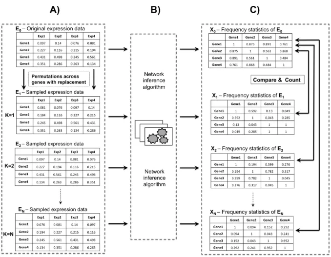
31
Figure 1.6: A). Common approach used to build a consensus network from multiple microarray experiments using a single inference method. B). Proposed approach to build a consensus network for one experiment using multiple inference methods. EXP indicates microarray experimental conditions; 1, 2 represents different network inference algorithms and N indicates the number of algorithms used.
By contrast to the well-established single inference method approach used in these studies, building a quantitative consensus network from multiple network inference algorithms using a single microarray experimental condition is still in its infancy (Figure 1.6B). Mendoza et al (Mendoza & Bazzan 2012), explored the benefits of consensus networks which includes BCEM to optimize the reverse engineering of GRNs on the same expression dataset. However, they focused on building consensus networks from only two network inference algorithms; Boolean networks and Bayesian networks. Indeed, generating an accurate consensus network, and more robust to experimental noise that in this fashion is the most discussed topic in laboratories (Bilal et al. 2015). There has been no detailed
quantitative analysis of consensus networks which requires further investigation. This is where we start this work, thus motivating us to combine the predictions generated from each network algorithm statistically to form an ensemble that delivers robust predictions for one experiment. The collective knowledge obtained by integrating multiple inference methods (the“Wisdom of crowds”) is greater than that conferred by any individual method (Marbach et al. 2012). Considering the advantages and disadvantages of each inference method is a critical part of this procedure.
1.6.1 Fishers combined probability test
Fisher’s combined probability test (FCPT) was proposed by R.A. Fisher (Fisher 1932) for combining p-values from a group of independent statistical tests - usually from multiple studies under the same null hypothesis. The null hypothesis states no treatment effect, and the p-values of each individual study are independent, uniformly distributed random variables that represent the probability of the observed significance level being attained in the experiment under the null hypothesis. FCPT has been previously employed in genomic research for combining p-values. For example, Hess et al. (Hess & Iyer 2007) successfully used this method to combine p-values from the probe level test of significance for detecting differentially expressed genes from Affymetrix microarray gene expression data.
The FCPT is defined below in the context of combining edges from multiple networks:
Fi =−2 log
j=1 n
∑
( )
Pij ≈ X22n(1.1)
Here, Fi signifies the combined p-value for a particular edge i, Pij represents the edge weight (p-value) for the jthhypothesis test (i.e. the jth network algorithm), and n corresponds to the number of independent tests performed (i.e. the number of network algorithms applied). The
33
score for a candidate edge is calculated by taking the product of the p-values computed from each network algorithm, then applying the negative logarithm (Fisher 1932). This measures the approximate chi-square distribution on scaling by a factor of two, with 2n degrees of freedom, X2
2n
.
Despite its simplicity, the FCPT has the potential to combine extreme probability values generated from independent tests, to deliver robust predictions (Hess & Iyer 2007). In addition to its simplicity, the major advantage of this method is that it allows the gene interaction weights to be standardized to a common scale, and provides probabilistic measures to detect if a gene interaction is significant. This motivated us to investigate its potential to solve the network inference problem.
1.7
Aims and Objectives
In this thesis, we aim to explore the use of consensus learning approaches as a means to enhance the quality and robustness of the predictions made by network inference algorithms for GRN reconstruction. The broader aim of this thesis is to provide a theoretical framework to evaluate some of the more popular qualitative and quantitative consensus techniques used for combining edge predictions from independent inference algorithms. More specifically, the novel contributions of this thesis are outlined below:
1. We developed a new network inference method, referred to as the quantitative consensus network method. This uses FCPT to combine the significance values assigned to each network edge by the inference algorithms to produce a consensus network. We provide evidence in this thesis that FCPT provides a robust and efficient inference method by applying it to a variety of in silico benchmark datasets (Chapter
3) and also to some real experimental datasets (Chapter 5). The development of the quantitative consensus network method involved the following:
o A non-parametric based random sampling algorithm was derived, in order to convert the statistical scores associated with each network edge to significance values (p-values) (Chapter 3).
o In order to control false positives, the single hypothesis testing strategy from FCPT was then further enhanced using a multiple hypothesis testing strategy - the False Discovery Rate (FDR) control for edge prediction (Chapter 3). 2. We also proposed two new scoring methods: module score and model score. Module
score quantifies biologically meaningful modular networks that show statistically significant association of its genes to a biological process, while model score quantifies the ability of a network algorithm to predict biologically relevant modular networks from in silico data (Chapter 4) and real experimental data (Chapter 5)
1.8
Thesis Overview
This thesis is organized into six chapters. An abstract is included at the beginning of each chapter summarising its content.
Chapter 1 provides a general introduction to the field of biological networks, which includes the motivation for the study and a description of its novel contributions.
Chapter 2 provides background and literature review of GRNs, whilst introducing the different reverse engineering techniques used in reconstructing GRNs. This chapter is further extended to review the existing qualitative and quantitative consensus learning methods - used to combine multiple network predictions - and to discuss statistical meta-analysis approaches in the field of bioinformatics and medicine.
35
Chapter 3 investigates a new network inference approach referred to as the quantitative consensus network. This is built on using the FCPT to integrate the predictions obtained from multiple inference algorithms. In this chapter, a new non-parametric algorithm was also presented which uses a random sampling approach by permutation analysis to transform the statistical scores associated with each network edge into significance values (p-values) in order to convert all predictions into a common metric. Furthermore, the consensus network by FCPT was tested and validated using a variety of in silico expression datasets for different experimental scenarios. We assess and discuss the potential advantages of consensus networks over individual networking methods, and compare existing qualitative and quantitative consensus techniques for robustness and efficiency.
Chapter 4 presents module and model scores by examining existing network inference algorithms for their ability to produce biologically meaningful hierarchical modular networks when tested with in silico expression data. Furthermore, the assumptions and limitations surrounding these scores were also described.
Chapter 5 examines the application of the new consensus network algorithm by FCPT to identify genome-wide regulatory interactions from real high-throughput expression data from a simple eukaryote. The performance measures achieved from FCPT were compared against those identified from other qualitative and quantitative consensus methods and other individual networking methods. Furthermore, this chapter presents modular and model scores for biologically meaningful hierarchical modular networks with real data.
Chapter 6 concludes the thesis. The limitations of this present study and the direction of future works are also discussed, relating back to the claims made in Chapter 1.
Chapter
2
2.
Background and literature review
Abstract
This chapter provides some background on the various types of existing network inference approaches currently used to study GRNs, further extending to provide a brief overview of the existing qualitative and quantitative consensus approaches (meta-analysis) currently applied for combining predictions from multiple network inference methods.
37
2.1
Modelling gene regulatory networks
The primary objective of modelling a gene regulatory network (GRN) is to identify the following types of interactions: 1) Physical (protein-gene) interactions – these occur between a transcription factor (TF - a protein) and its target genes, i.e. TF binding to a sequence motif on the promoter of a target gene; 2) Influence (gene-gene) interactions – such interactions encapsulate a causal relationship between two genes by relating the expression of a gene i to that of a gene j (Bansal et al. 2007).
In the last decade, many network inference approaches have been developed which are used to reconstruct GRNs from microarray gene expression data. The methods predominantly used are broadly classified into the following categories:
1. Information theory models 2. Bayesian network models 3. Differential equation models
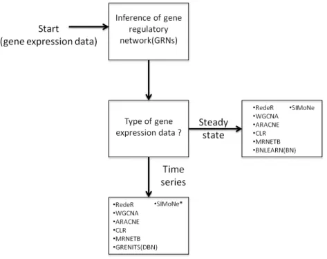
Depending on the type of gene expression data available, the network inference algorithm can be chosen accordingly to predict regulatory interactions, as shown schematically in Figure 2.1.
Figure 2.1: Flow chart for choosing a suitable network inference algorithm depending on the type of gene expression data used. (BN): Bayesian network; (DBN): Dynamic Bayesian network; (*): Algorithm that requires to change parameters depending on the type of the data.
2.1.1 Information theory models 2.1.1.1 Correlation networks
One of the simplest network modelling approaches is the correlation based network (Stuart et al. 2003). Here, the interaction between each pair of genes is weighted using the Pearson or Spearman correlation coefficients computed from their expression profiles, resulting in an undirected network. Two genes are characterised as connected only if the correlation coefficient between their expressions is above a specified threshold. The value of the threshold determines the sparseness of the network. These networks are also known as co-expression networks and capture the linear dependence between genes. A correlation coefficient close to zero is a strong indicator of independence between any gene pair.
39
The Pearson Correlation Coefficient (PCC) rxy is calculated between gene x and target gene y as shown in equation (2.1): rxy = n xiyi i=1 n
∑
− xi i=1 n∑
yi i=1 n∑
n xi2 i=1 n∑
−( xi i=1 n∑
)2 n yi2 i=1 n∑
−( yi i=1 n∑
)2 (2.1)In this equation, n represents the number of experimental sampled measurements of gene x and gene y. Correlation coefficients ranges between +1 and -1. A high positive correlation indicates high similarity between the expression profiles of two genes (x and y). While, high negative correlation indicates the expression profiles of both genes are in opposite direction. Spearman’s Rank Correlation Coefficient !xy instead uses ranked expression profiles to
calculate the distance measure between genes x and y using PCC as specified in equation (2.2) ρxy =1− 6 di 2 i=1 n
∑
n(n2 −1) (2.2)Here, di signifies the difference in rank order between genes x and y over n sample measurements.
The correlation based benchmark algorithms used for consensus analysis are RedeR and WGCNA that are described below.
RedeR
The RedeR algorithm reconstructs a hierarchical nested network using gene expression data (Castro et al. 2012). It manages and organizes network data structure using mixed graphs in two different layers. In the first layer, a directed acyclic graph (DAG) is defined where each
node has one parent, multiple branches, and no feedback cycles. The second layer connects the DAG components to produce a hierarchical topology in an undirected graph (UDG), as illustrated in Figure 2.2.
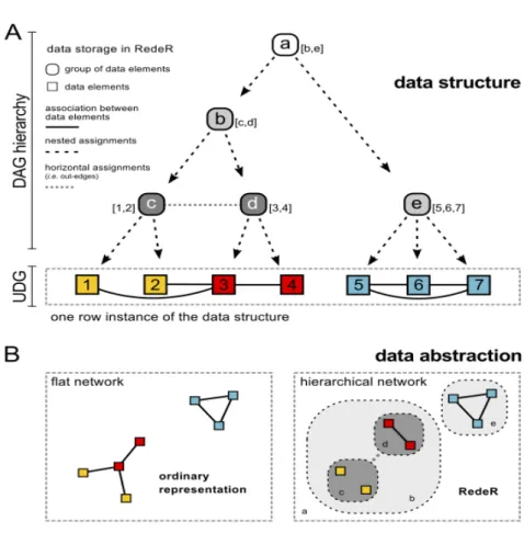
Figure 2.2: Hierarchical modular network structure from RedeR. A) Data structure connecting a directed acyclic graph (DAG) and an undirected graph (UDG) in two different layers. Here, letters a,b,c,d and e denote modules and numbers 1 to 7 represents genes. B) Data abstraction outlines the hierarchical network (right) in contrast to the flat network (left). The figure was adapted from (Castro et al. 2012).
Euclidian distance was calculated to derive a dendogram from complete linkage clustering for reconstructing the hierarchical network. The associations between co-expressed genes were calculated using Spearman’s rank correlation coefficient, !, as defined in equation (2.2).
41 WGCNA
The WGCNA (Weighted Correlation Network Analysis) algorithm produces a modular network of highly correlated genes using an unsupervised clustering technique in a two step process (Langfelder & Horvath 2008).
In the first step, the signed co-expression similarity network Sij is defined and utilized as an intermediate quantity to calculate a weighted adjacency matrix Aij. The Sij network is computed using co-expression (using Pearson Correlation Coefficient) measures that identify interacting patterns between gene i and gene j. The weighted adjacency matrix is calculated by raising the co-expression similarity Sij to a soft power β:
Sij = 1+corr(xi,xj) 2 (2.3) Aij = S β ij (2.4)
The values of Aij range between 0 and 1, denoting minimum and maximum edge strength respectively between node i and node j. β was fixed at its default value of 6 in our analysis. The correlation coefficients were transformed back to derive PCC values using the modified equation below. 1 2 (1/ ) − = ij β ij A r (2.5)
The second step identifies functional modules associated with the co-expression network using a hierarchical clustering method. The dendogram associated with these hierarchical clustering branches correspond to modules. To derive the desired number of modules, the hierarchical tree was cut at a desired height and correspondingly the optimized Module Eigen dissimilarity threshold was fixed (Langfelder & Horvath 2008).
WGCNA has successfully been used to determine cluster modules from microarray gene expression data in the yeast cell cycle, the human brain and the mice liver (Langfelder & Horvath 2008).
2.1.1.2 Mutual information
Mutual information based networks rely on the entropy scores (known as Shannon’s entropy) computed from gene expression measurements that indicates how much information obtained from the expression profile of one gene predicts the behavior of the other gene (Steuer et al. 2002). Like correlation analysis, mutual information determines the degree of statistical interconnection between two random gene variables. However, mutual information captures the degree of non-linear dependence between two genes based on their discretised expression profiles. Given two random variables Xi and Xj representing the expression levels of two genes i and j, the mutual information (MI) between gene i and gene j is defined as
MIij =Hi+Hj −Hij (2.6)
where
Hi= p X
(
i =x)
log2 p X(
i =x)
x∑
(2.7)is the entropy for the expression of gene i - a measure of information content in the distribution pattern of expression levels across measurements – and
Hij =− p X
(
i =x,Xj =y)
log2 p X(
i =x,Xj =y)
y
∑
x∑
(2.8)is the joint entropy for genes i and j. Entropy is calculated using discrete probabilities, and therefore applies histogram techniques. The entropy is higher when the distribution of gene expression is more randomly distributed and reaches a maximum when distribution is
43
uniform. From this definition, the two random gene variables Xi and Xj are statistically independent if the MI is zero, i.e. if the joint entropy Hij=Hi+Hj, meaning that p(Xi=x,Xj=y)=p(Xi=x)p(Xj=y). A higher MI indicates that the two gene variables are
non-randomly associated.
The mutual information derived statistic scores by weight are applied by network inference algorithms like ARACNE (Algorithm for the Reverse engineering of Accurate Cellular Networks) (Margolin et al. 2006), CLR (Context Likelihood to Relatedness) (Faith et al. 2007), and MRNETB (Maximum Relevance Minimum Redundancy Backward) (Meyer et al. 2010) to study large scale regulatory networks.
ARACNE
ARACNE (Algorithm for the Reconstruction of Accurate Cellular Networks) identifies the transcriptional regulatory network (TRN) between genes and their products using microarray gene expression data (Margolin et al. 2006). ARACNE predicts the association between genes through statistical dependency in two main steps.
In the first step, ARACNE derives a MI matrix, Mij=MIij for all input pairs of genes i and j in the expression dataset using the definition in equation (2.6). The gene expression data is continuous, so is discretized with the equal width binning method. The empirical probability distribution estimator for the assessment of a mutual information score is applied using the function build.mm with the number of bins set to n, where n denotes the number of experimental samples (Meyer et al. 2008).
The second step is a pruning procedure based on the Data Processing Inequality (DPI). The DPI is formally defined using a triplet of nodes {Xi;Xj;Xk}, where gene Xi interacts with gene Xj through gene Xk (Xi ! Xj ! Xk) then the edge that is weakest, which is considered as an indirect interaction, say{Xi;Xj} is removed if the mutual information weight
is below min{Mik,Mjk}-eps, where eps is a numerical threshold that is set to 0.15. The eps was relaxed from the default (0.05) as it was observed to be too stringent in our study. ARACNE has been successfully applied to study TRNs in human B cells and has outperformed Bayesian networks and several other inference methods (Margolin et al. 2006).
CLR
The CLR (Context Likelihood to Relatedness) (Faith et al. 2007) algorithm is built upon a MI-based relevance algorithm that is primarily used for clustering (Butte & Kohane 2000). The CLR algorithm has two main steps. In the first step, it calculates the MI matrix, Mij, for all input pairs of genes i and j in the expression dataset (as in ARACNE). In the second step, the algorithm eliminates false interactions by computing Z-scores. For each input pair of genes i and j, a Z-score, Zij is calculated from an empirical MI density for all regulators of the target gene Zj and an empirical MI density for all targets of the regulator gene Zi. CLR identifies possible interactions whereby MI values are significantly above the empirical distribution of MI values. That is, instead of considering mutual information values Mij for random gene variables Xi and Xj , it calculates Z-scores, Zij = Zi2+Z2j where,
In equation (2.9), µi represents the mean and σi the standard deviation of the empirical distribution of mutual information values {Mik; k=1,…,n}. The CLR algorithm has been successfully applied to decipher the E.coli TRN (Faith et al. 2007) .
Z
i=
max
k0,
M
ik-
µ
iσ
i!
"
#
$
%
&
(2.9)45 MRNETB
The MRNETB (Maximum Relevance Minimum Redundancy Backward) algorithm is an improved version of MRNET that depends on the feature selection strategy known as MRMR (Maximum Relevance Minimum Redundancy). That is, to select genes, a sequence of supervised learning is applied by MRMR, wherein each gene is played as a regulator. For example, consider a supervised learning task, where X is a set of input variables and Y is the output. A score, S is used to sort X by rank, calculated using the difference between maximum relevance (MI of output gene variable Y) and minimum redundancy (mean MI of the penultimate ranked gene variable X). The higher ranked variables indicate direct interactions whereas lower ranked variables are considered as indirect interactions. Specifically, MRMR starts by selecting a variable Xk that has the highest mutual information
Mkj to the target Xj. It then selects the variable Xi that has high mutual information Mij to the
target Xj and at the same time has low mutual information Mkj to the previously selected variable. A major limitation of MRNET is that it used forward selection strategy that strongly depends on the first variable selected (i.e. variable having the highest MI with the target gene). If the first variable selected is not a true target then maximizing MRMR may not be advantageous. In contrast, MRNETB uses a backward elimination combined with sequential search to rank all candidate edges (Meyer et al. 2010).
MRNETB infers edges in a two-step process. In the first step, it estimates MI values same as in ARACNE and CLR. In the second step, MRNETB initiates the selection of edges from a set XSj through backward elimination employing the MRMR principle to rank features using
the score Sj containing all variables (XSj ⊆ X \ Xi) and then removes Xi iteratively that
actuates maximal increase of the XSj score until the termination criteria is reached i.e. when
The enhancement of the process is achieved by sequential replacement, where at each step, the status of selected and non-selected variables is swapped so that the maximal increase in the objective function (i.e. XSj score) is reached. MRNETB algorithm was implemented using
the minet package (Meyer et al. 2008), and it has been previously applied to study SynTReN derived and DREAM4 challenge benchmark da