MCC-IMS data analysis using automated spectra processing and explorative visualisation methods

(1)

MCC-IMS data analysis using automated

spectra processing and explorative

visualisation methods

Zur Erlangung des akademischen Grades eines

Doktors der Naturwissenschaften an der

Technischen Fakultät der Universität Bielefeld

vorgelegte Dissertation

von

Alexander Bunkowski

15. August 2011

(2)

(3)

3 Alexander Bunkowski

Adalbert-Stifter-Str. 4 33613 Bielefeld

[email protected]

Supervisors: Prof. Dr. Jens Stoye

PD. Dr. Jörg Ingo Baumbach

(4)

(5)

Summary

Ion Mobility Spectrometry (IMS) is a method to characterise chemical substances on the basis of velocity of gas-phase ions in an electrical field. The data resulting from an IMS measurement is a number of spectra sorted by retention time. Each spectrum contains a series of values and each value represents the amount of ionised molecules at one specific drift time. Recent advantages in the field of Ion Mobility Spectrometry lead to an highly increased amount of data per measure-ment as well as measuremeasure-ments per experimeasure-ment. Due to the usage of a Multi-capillary Chromatographic Column (MCC) as pre-separation tech-nique the task of analysing and interpreting the resulting data com-pletely changed and now includes a pseudo coloured image in addition to the classic spectra data. Analysing and comparing a high number of these images and their corresponding spectra is almost impossible and extremely time consuming with the methods used so far.

Different methods for spectra processing, data analysis, visualisa-tion and project management were developed and combined in one software called ’IMS Peaklist & Heatmap Explorer’ (IPHEx) to challenge this task. IPHEx is the first software system supporting the analysis, management, and visualisation of large amounts of MCC-IMS measure-ments in parallel. It is currently used for the investigation of metabolo-mic experiments with a focus on the analysis of exhaled air, headspace samples of cell and bacteria cultures, as well as general screening of ambient air. While the main methods of IPHEx are designed to pro-cess three dimensional data obtained from different MCC-IMS devices, it also handles GC-MS based data for comparison and substance iden-tification as well as several other information obtained from flat and Excel files. It became the standard analysis platform at the

(10)

Institut für Analytische Wissenschaften ISAS e.V._{for MCC-IMS data and}

showed its potential during the examination of experiments performed in cooperation with theLungenklinik Hemer - Zentrum für Pneumologie und Thoraxchirurgie_{, the} University Göttingen - Department of Anes-thesiology, Emergency and Intensive Care Medicine_{, the}Charité - Uni-versitätsmedizin Berlin _{and several others. It is also used for}

exper-imental purposes at the Korea Institute of Science and Technology, Saarbrücken _{and the} B&S Analytik GmbH, Dortmund_.

The application to many different experiments and tasks demon-strates that the requirements have successfully been addressed and the software and therefore the underlying methods and concepts are suited to analyse large amounts of IMS data in an efficient way. With IPHEx, a complete analysis environment exists, which offers a solution for all analysis, management, and visualisation tasks which are nec-essary to perform a comprehensive investigation of large amounts of MCC-IMS data.

(11)

CHAPTER

1

Motivation and overview

Ion Mobility Spectrometry (IMS) is a method to characterise chemical substances on the basis of velocity of gas-phase ions in an electrical field.

The first developments in the field of molecule detectors and ion-mobility were done by the U.S. Army during the 1960s to detect nerve agents. With a type of ion mobility cutoff filter, ions over a certain size which are typical for nerve agents could be distinguished from smaller ions, commonly formed in clean air. An overview of the different con-tracts and patents which were set up during this time is given in the book Ion Mobility Spectrometry_{of Eiceman and Karpas [1].}

When the first civil research programs in Ion Mobility Spectrometry for chemical analyses started in 1970 at the University of Waterloo in Canada, a single spectrum per measurement could be obtained in about five minutes [2]. Further major developments were performed by Baim and Hill in 1982, allowing among other advantages, the usage of gas chromatographic methods to pre-separate a sample and thus the recording of several spectra per measurement [3].

In 1971, the first modern breath tests were performed by Linus Paul-ing by detectPaul-ing volatile organic compounds (VOC) in cryogenically concentrated samples of human breath. Assays using gas chromatog-raphy/mass spectrometry have since identified more than 3000 differ-ent VOCs in human breath [4].

The here presented work was performed at the ISAS Leibniz-Institut für Analytische Wissenschaften - ISAS - e.V. _{which started research}

in the field of Ion Mobility Spectrometry in 1991. Until 1996 no

(12)

separation technique was used and thus only single spectra recorded and investigated. With the first usage of a Multi-capillary Chromato-graphic Column (MCC) to perform a pre-separation, complex mixtures containing many different chemical compounds could be analysed. Several hundred spectra per measurement were recorded from now on and as a result of that, new methods were demanded to handle, anal-yse, and visualise this greatly increased amount of data. About one second is needed to record a single spectrum, and depending on the aim of an analysis about five hundred spectra are recorded per sample, resulting in a record time below ten minutes per measurement. This low time enables to record many measurements per project, which further increases the amount of data to handle. After an initial intro-duction of the IUPAC-Format for IMS spectra [5] this data was stored in an specialised data format for GC/IMS applications [6, 7].

To cover these requirements, different methods for spectra process-ing, data analysis and visualisation were developed. All of these were combined in one Software called ’IMS Peaklist & Heatmap Explorer’ (IPHEx) to enable a fast and coherent analysis of IMS data with all its associated information.

The following chapters describe the methods and concepts which are necessary to enable the analysis of MCC/IMS data as well as the result-ing software system and the application of it. Chapter 2 begins with an overview of the scientific background of IMS and its applications. It provides information about the origin of the investigated samples, de-scribes the used techniques and devices and gives an overview about the data and the general analysis procedure.

Chapter 3 analyses the requirements which have to be addressed to enable a successful MCC/IM data analysis and leads to a number of different data structures, processing approaches, and graphical user interfaces which have to be established.

The structure of Chapter 4 follows the order of necessary methods to enable the data analysis from spectra pre-processing to peak detec-tion and data analysis, concluding with methods for visualisadetec-tion and exploration.

Chapter 5 describes the IMS Peaklist and Heatmap Explorer _IPHEx,

which was built to apply the developed methods to IMS data and visu-alise, manage and compare their results. It starts with a description of the different data structures that are created and used by the software and a detailed description of the user interface and its different com-pounds. It also includes a description of the general workflow of IPHEx and shows how the different parts of the software are typically applied to perform an IMS data analysis with IPHEx.

(13)

9 In Chapter 6 examples of metabolomic experiments and their analy-sis using the IPHEx software are described. Using the IPHEx software system, a detailed and fast analysis of large data sets and an integra-tion of various existing informaintegra-tion is possible, which is necessary to analyse these kind of metabolomic experiments.

A discussion of the System is provided in Chapter 7 followed by an outlook in Chapter 8.

(14)

(15)

CHAPTER

2

Background

This chapter introduces the scientific background of IMS and its appli-cations. The different terms, areas and instruments which are needed to understand the basics of this thesis are pointed out. The first part describes the general field in which this work is settled and provides information about the origin of the investigated samples. It is followed by a description of the used techniques and devices and concludes with a specification of the generated datasets and an overview of the data analysis procedure.

2.1. Metabolomic analysis

Metabolites are substances which are created and/or used by the meta-bolism of an organism. The study of chemical processes involving metabolites provides a view inside the biochemical status of a cell or an organism. All metabolites of an organism are termed metabolome. The qualitative and quantitative analysis of all metabolites, present at one specific time in an organism, a tissue or a cell, is termed meta-bolomics [8]. It can give insight into the functions of unknown genes, cell systems or organisms, with respect to the response to external stimuli. By comparing metabolite occurrences and their levels in two or more sets of samples, significant differences may be identified. For example comparing metabolites from subjects suffering from a disease and healthy subjects can help to develop new diagnoses and treat-ments.

(16)

These comprehensive analyses are based on modern analytical and computational approaches and can be divided into two general steps. At first, the biological samples have to be extracted, eventually derivati-sised and measured with a proper analytical method. The second step is the identification of the measured analytes with the use of existing databases and the comparison of different samples using computa-tional approaches. For global metabolic profiling, the most popular analytical methods used today are based on mass spectrometry, es-pecially in combination with gas or liquid chromatographic systems [9, 10].

In this work, volatile organic compounds are analysed to retrieve information about metabolites by screening either the exhaled air of humans (breath analysis), or the gas space above a biological sample (headspace analysis).

2.1.1. Breath and headspace analysis

Blood and urine analysis are standard techniques in medical examina-tions for various tasks and deliver information about the health status of a patient. During the last years several studies showed that exhaled air is a carrier of information about the metabolic state, including infor-mation about infections, medications, and diseases [11, 12, 13]. In the majority of present studies, a non invasive method for early diagno-sis or therapy monitoring should be developed by identifying disease-specific biomarkers in the breath of patients.

Headspace analysis is the analysis of all chemical compounds present in the gas space above a sample. A solid, liquid or gas sample is recorded and used for the determination of volatile organic compounds. This technique has evolved over many years and gained worldwide ac-ceptance for example to analyse blood and urine as well as residual solvents in pharmaceutical products.

The primary aim of these analyses in this context is to support and extend the field of breath diagnostics with laboratory studies of bio-molecules at comparatively low pressure. For example the identifica-tion of volatile organic compounds which are caused by clinically im-portant bacterial species (see 6.2) under controlled laboratory condi-tions can help to determine an infection with the respective bacterium of the human lung. Furthermore the metabolic profile of lung cancer cell lines can be compared to those from normal lung cells to support the task of diagnosing lung cancer effectively. Other applications, for example the comparison of the metabolome of cells grown on different medium, or under different experimental conditions are possible.

(17)

2.2. Ion mobility spectrometer ₁₃

Existing analytical methods used to perform breath and headspace analysis based on mass spectrometry are gas chromatography mass spectrometry (GC-MS) [14, 11], proton transfer reaction mass spec-trometry (PTR-MS) [15, 16], and selected ion flow tube mass spectrom-etry (SIFT-MS) [17, 18]. Beside these mass spectromspectrom-etry based ap-proaches there also exist different types of sensors [19, 20, 21, 22, 23], electronic noses [24, 25], and ion mobility spectrometry which was used in this work and is described in detail in the following section.

The IMS technology is very well suited to perform breath analysis because of several different facts:

Humid air can be analysed directly, which is a major problem for many other analytical approaches. The detection limit goes down to the level of picogram per litre.

A relatively low technical expenditure is necessary for the con-struction of an IMS, which directly results in lower costs of the device compared to the mass spectrometry based methods. The small size, low weight and power consumption as well as the

short time needed to acquire a measurement are further practical advantages of the technology.

Due to these facts, an installation and usage of the IMS device inside a hospital and thus a direct sampling of the breath is possible. This negates the influences of adsorbents or tedlar bags on the sample which are otherwise needed to transport a breath sample to a labora-tory. Even ambulant examinations and usage at general practitioners are possible and will become more likely once the technology develops further.

2.2. Ion mobility spectrometer

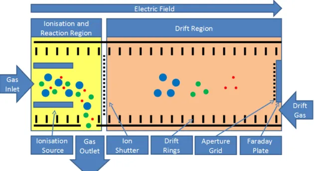
The term ion mobility spectrometer refers to the operating principle of the device. The gas phase ion mobilities of analytes are measured by ionising the gas and moving them under ambient pressure with a weak electrical field towards a Faraday plate after passing an electrical ion shutter (see Figure 2.1).

The measurement starts when the sample is brought into the ioni-sation and reaction region. The different molecules are ionised using a 63N β_{-radiation source. While the ion shutter is closed the probe}

leaves the reaction region through the gas outlet. During a short open-ing stage of the shutter a small amount of the ionised probe is brought into the drift region. Under the influence of an electrical field the ions

(18)

Figure 2.1.: _{IMS with closed ion shutter and a probe in the drift region.}

The sample enters the device trough the gas inlet on the left side and moves towards the faraday plate at the right side.

drift towards the Faraday plate at the end of the drift region and col-lide with drift gas molecules coming from the opposite direction. Due to this, the ions are decelerated in a varying manner depending on their structure and reach a steady drift velocity. In the ideal case, if no chemical reactions take place, the ions separate into different clus-ters and reach the Faraday plate. There, the ions are neutralised upon collision, causing a current flow of 10 to 1000 pA, which is amplified and converted into voltage. This time depended current is measured during an interval of half the shutter opening time and is called the ion mobility spectrum. The drift velocity (_d_{, in units of cm/sec) normalised}

to the strength of the electric field (E_{, in units of V/cm) is termed the}

ion mobility:

_d=K E _(2.1)

The proportionality coefficient, K, is called the mobility coefficient of the ion in units of cm2V−1sec−1_{. Calculated mobility coefficients}

are usually normalised to the reduced ion mobility (k₀_{) as shown in}

Equation 2.2 with the values P₀ _{= 760 Torr and} T₀ _{= 273 Kelvin while}

P and T are the respective measured values inside the drift tube. T is temperature in Kelvin and P is pressure in torr of the gas atmosphere through which the ions move.

(19)

2.2. Ion mobility spectrometer ₁₅ k₀=K T₀ T P P₀ (2.2)

Reactant ions are formed continuously by the radioactive ionisation source and are brought into the drift region due to the electrical field. When no analyte molecules are available, the reactant ions move to-wards the Faraday plate and form a spectrum which contains the Re-actant Ion Peak (RIP) [1].

2.2.1. Experimental setup

The detection of metabolites in complex mixtures like headspaces of cell and bacteria cultures as well as human breath results in a high number of detected analytes.

Figure 2.2.:_{Complete experimental setup of an IMS coupled to a}

multi-capillary chromatographic column and a sample loop to al-low the recording of headspace and breath sample under controlled conditions.

To avoid overlapping of the signals and to improve the separation and identification capabilities, a multi-capillary chromatographic col-umn (MCC) is used for separation. To keep the speed of the pre-separation constant under varying conditions, a heating unit is used to stabilise the temperature at a constant value. Furthermore, a sam-ple loop is used to buffer the samsam-ple and transport it into the MCC at a constant pressure, using a drift gas (Figure 2.2). The integration of the MCC increases the recorded data from one spectrum per sample

(20)

to a set of several hundred spectra. Thus a third parameter called retention time is added to each signal, in addition to the 1/ k₀ _and

sig-nal intensity. In general, an asig-nalysis with this experimental MCC-IMS setup consist of a number of measurement sequences recorded under different experimental conditions or taken from different persons. A sequence consist of an instrumental blank, a sample of the room air or the medium, and the measurement of the exhaled air or headspace sample. The instrumental blank is taken to exclude general contamina-tion of the device and ensure that no substances are left from previous samples. A room air or medium sample is analysed to identify sub-stances which occur in the ambient air or medium and thus are taken to account afterwards when analysing the sample. The third and most important record is the probe sample, carrying information about the volatile organic compounds of the target. The comparison of these measurements to identify analytes and determine similarities and dif-ferences between classes of measurements is the general aim of an experiment.

2.2.2. MCC-IMS Data

The data resulting from an MCC-IMS measurement is a file with a number of spectra sorted by retention time. Each spectrum contains a series of values and each value represents the amount of ionised molecules at one specific drift time.

Each spectrum consist of a number of single scans which are aver-aged to one spectrum (Figure 2.3). The time needed for one single scan is 100 milliseconds, typically 10 scans are used to build one spec-trum which leads to an acquisition speed of one specspec-trum per second. This is necessary to improve the noise to signal ratio and thus separate weak signals from noise.

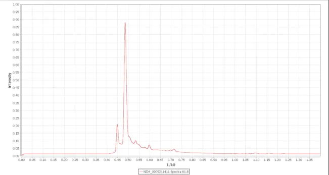
Typically a measurement consist of 500 single spectra, where each of them contains 2000 values. This leads to a set of one million data-points, where each datapoint consist of the three parameters retention time, drift time and intensity. Each spectrum contains a dominant sig-nal, called the Reactant Ion Peak which is caused by the ionisation source of an IMS and further peaks which contain information about the measured substances of the sample.

(21)

2.3. Data analysis procedures and related work ₁₇

Figure 2.3.:_{One IMS spectrum, averaged over 10 single scans. The}

x-axis shows 1/ k₀ _{, while the y-axis is ued to display the} signal intensity.

2.3. Data analysis procedures and related

work

In 1991, when the first IMS was used at the ISAS, no MCC was used for pre-separation and thus only one spectrum per measurement was recorded [26]. The resulting spectrum, containing about 2000 data-points, was investigated with common available software applications like Microsoft Excel and Origin (www.originlab.com). Due to the low complexity, no dedicated software was needed. With the application of the MCC in 2001 [27] the amount of data highly increased, since multiple spectra per measurement were recorded and new strategies to analyse the datasets were developed. A first step was to convert the set of single spectra into a matrix and visualise it with the help of Origin as a pseudo colorised map. With a combination of these maps and selected single spectra the analysis was done completely manu-ally. A second factor which increased the amount of data was a change of the experimental focus in 2002 from single compound analysis [28] to complex applications like process analytics [29], emission of sur-faces [30], cell and bacteria cultures [31] and the analysis of exhaled air. Due to the complexity and aims of those experiments, more mea-surements per experiment were recorded and compared with respect to external stimuli. Analysing and comparing a high number of these

(22)

images and their corresponding spectra is almost impossible with the methods used so far.

The analysis of MCC-IMS data can not be performed with available spectrometric software for MS with chromatographic columns, since the structural differences are too big. This is mainly because GC-MS/LC-MS analysis is based on investigating two dimensional total ion count spectra and using the mass decomposition spectra to identify compounds at specific locations, while the MCC-IMS data needs to be analysed based on a three dimensional, image like spectrum. On the other hand, existing image analysis tools are hard to apply because they lose the information of the underlying spectra.

Several people were acquired as diploma, master, and PhD students to investigate those problems. The first one was Sabine Bader who worked on the identification and quantification of peaks in spectromet-ric data [32, 33]. After her work, several diploma and master theses were set up by the ISAS in cooperation with Dortmund University and Bielefeld University to find solutions for the data analysis process. As a result of this process, one software called BBImsAnalyse _was

devel-oped and will be described in the following section.

2.3.1. BBImsAnalyse Software

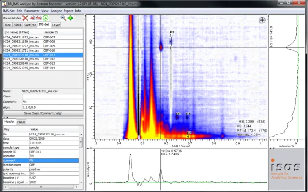
The BBImsAnalyse Software was developed by Bertram Bödeker during his diploma thesis [34] at the ISAS and was the first software explicitly designed for MCC-IMS data analysis based on a heatmap representa-tion. It offers preprocessing functions a well as the possibility to setup a basic annotation layer for regions. It is also possible to compare different measurements based on layers with an integrated tool and export resulting values to an excel file for further analysis.

Visualisation

Within the central window of 2.4, the whole chromatogram from the data file is shown as two-dimensional-plot, where the signal height is colour-coded.

A single peak can be marked by a mouse-click with a cross line. Thus, the single spectrum at the selected retention time becomes available in lower window and one single chromatogram at the se-lected ion mobility in the window on the right side.

Also in the lower window the parameter of the data point at the cur-rent mouse position like 1/ k₀ _{, k0, and the intensity are visible.}

Analo-gous, in the right window the retention time at the position of the cross line is shown.

(23)

2.3. Data analysis procedures and related work ₁₉

Figure 2.4.:_{Screenshot of the BBImsAnalyse software user interface.}

A heatmap in the centre visualises one measurement, the bottom and right parts show representation of single spec-tra which were selected.

To compare different peaks, it is necessary to mark the peak position in the central window manually one after the other [35].

Peak comparison

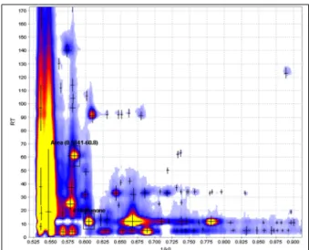
The Software enables the selection of an area in the heatmap directly and the search of the same area in further measurements. The find-ings can be visualised as shown in Figure 2.5 together with some peak characteristics. In this case eucalyptol as an analyte frequently found in human breath samples was used to illustrate the application of the peak comparison procedure [36].

2.3.2. VisualNow

The BBImsAnalyse Software was further developed, improved, used, and renamed to VisualNow by the B&S Analytik GmbH, Dortmund _[37,

38]. Those improvements include the possibility to analyse and com-pare an increased amount of measurements and apply statistical val-ues as well as Box-and-Wisker-Plot visualisation to the results.

(24)

Figure 2.5.: Peak comparison of a marked area in 20 different samples of human breath ordered by signal intensity from the up-per left (highest value) to lower right (no relevant signal intensity) [36].

(25)

CHAPTER

3

Requirements

The previous chapter showed that current developments in the appli-cation of the MCC-IMS technology make an analysis with existing soft-ware tools complicated and time consuming. With the change from a single spectrum per measurement to several hundreds and a drasti-cally increasing number of measurements per experiment, new con-cepts for data handling and analysis need to be discovered.

Two main requirements can be formulated, regarding the current de-velopments and problems.

A method needs to be found to enable a combination of spectra based and image based analysis features in one environment. A high number of measurements and analysis results need to be

stored and maintained in a project oriented way.

To achieve both goals, they need to be analysed in detail as each of them consists of several tasks to solve and require the design of different data structures, processing approaches, and graphical user interfaces.

3.1. Spectra and image analysis

The data recorded by an MCC-IMS is always effected by a certain amount of noise. To improve the visualisation and all subsequent anal-ysis, filtering methods need to be applied to reduce these negative

(26)

effects. Since there exist several different MCC-IMS devices, and small differences of device parameter and ambient effects can influence the measurement, it is necessary to ensure that the data can be com-pared to each other. Therefore different alignment and baseline cor-rection methods should be applied. The reactant ion peak (RIP) which is caused by the ionisation source of an IMS needs to be regarded in de-tail, because it dominates every spectrum and can overlay important signals, which causes problems in further analysis and visualisation. The key information every IMS measurement contains is the informa-tion about the type and amount of substances in the sample. Therefore functionality to annotate, identify and quantify peaks needs to be pro-vided. In the ideal case, the data matrix is transformed into a list of all contained substances which forms the fundament for all subsequent analysis. To enable this and provide a general analysis environment for MCC-IMS measurements, visualisation methods are required. Since the data contains more image like information than other spectrometric methods but also contains more value based and axis depended data than standard image processing tasks, a combined analysis needs to be done based on both, the generated image and the individual spec-tra. A visual analysis environment needs to provide an overview as well as functionality to zoom and filter, and provide details-on-demand [39].

3.2. Project and result management

All measurements are typically taken in an experimental context, mean-ing there exist several measurements that are related to a specific analysis goal and thus need to be compared. Therefore, a list of all measurements which belong to one experiment should be provided by a project managing interface. All measurement files contain cer-tain parameters and labels which were assigned during the sample recording and should be provided within this project manager as well. Additionally there often exists external information which is related to the measurements. In case of headspace samples this can be infor-mation about the medium, type and number of cells or age for ex-ample. When analysing exhaled air, there typically exists information about the respective person, like type of disease, gender, age and values that originate from blood or similar analysis. This additional information is important for further analysis and can be divided into two general types. The first one to group the measurements into dif-ferent classes to compare those classes against each other, and the other one to include additional parameters for the analysis. Such

(27)

in-3.3. Required data formats and concepts ₂₃

formation is termed meta information and needs to be displayed in the project manager. The information about the type and amount of substances in each sample should be included in the project manager view as well. Therefore a procedure needs to be developed to select specific substances or regions of measurements and provide methods to sort, filter and compare them.

Combining all this information in one view would allow a structured analysis of a large set of measurements. Since the amount of data to display can become large, techniques to select relevant information and hide currently unnecessary data need to be included. For those experiments with a high number of measurements it is important to avoid the need of displaying every single measurement and analysing it by hand and one by one. Only a few measurements should be viewed as representatives of their respective classes or even one for the whole experiment. Methods should be provided to identify and filter peculiar measurements and highlight them for further investigation. Further-more peaks should be detected automatically because labelling them by hand can be extremely time consuming if not impossible in large projects. Nevertheless a software system should provide a method to perform a manual validation and editing of the peaks to correct possi-ble errors and handle unexpected cases. The last point which should be regarded to reduce the time needed to analyse projects with a high number of measurements is that in many cases for similar projects there exists a subset of necessary analysis and annotation tasks which are identical. Therefore, functionality should be provided to transfer information between projects and compare them.

3.3. Required data formats and concepts

The analysis of the requirements lead to a number of necessary data formats and concepts which need to be handled and provided.

3.3.1. Measurement files

The first and most obvious necessary data format is a representation of the measurement file itself. The file consists of a header which con-tains many information about the device and measurement param-eters as well as some information about the recorded sample which can be created while recording it. Furthermore it contains a list of all recorded spectra with information about retention time, drift time and spectra number. Each of those spectra is a list of measured val-ues. The format of this file is a simple character separated values file

(28)

whose structure was defined by the ISAS. A data object needs to be created which enables access to the header information and all spec-tra together with the retention time and drift time coordinates.

3.3.2. Peak lists

A second data structure is needed to determine and compare the type and amount of substances in each sample. This structure called peak list needs to cover information about all peaks that occur in one mea-surement and is represented as a list of peaks. The parameter to de-scribe one peak are peak position, consisting of retention time position and drift time position, the area of all elements belonging to a peak, the volume and the maximal intensity of the peak. As this information is very important for the analysis and an exchange with other software tools may be wanted, a simple exchange format is needed. Therefore peak lists should be saved in a tab separated text file where each line represents one peak and thus contains all necessary parameters sep-arated by tabs. A header as first line is needed to define the type of parameter in each column.

3.3.3. Area annotations

The identification of a peak should be treated separately from the peak lists, since the parameter of a detected peak can not change, but the assignment of a substance name to a peak can change or become more precisely once an analysis progresses or the databases for iden-tifications grow. The position parameter of identified substances typ-ically contains a small range of drift and retention times where they can occur. Therefore an annotation type needs to be defined which contains the name of the substance, describes the position of a sub-stance in form of a retention time index and a drift time index, as well as tolerance values for both indices. Existing annotations need to be read from external locations and a mechanism to define and save such annotations to use them in further projects should be established.

3.3.4. Heatmap images

A visual representation of the data is necessary to explore and work with the measurements, visualise peak lists, and define annotations. A suitable concept for this task is the generation of a heatmap image. A heatmap is a graphical representation of data that offers a possibil-ity to visualise three parameters of a large number of data objects in

(29)

3.3. Required data formats and concepts ₂₅

Figure 3.1.:_{Example of a heatmap created from a MCC-IMS}

measure-ment with labeled peaks and annotations.

one image. Using this method, two parameter of an object are used to determine the position of a pixel inside the image while the third parameter is encoded by colour. The term heat _{is used because}

typ-ically low values are represented by blue colour and implicate a low temperature while higher values are represented by red and yellow colours which are often associated with high temperatures. Using the retention time and drift time indices of all values of a measurement as coordinates and the intensity values to encode the colour enables the visualisation of a whole measurement as one image. Furthermore peak coordinates can be drawn on this image and annotations to iden-tify and compare peaks can be defined. An example of a heatmap with peak coordinates and annotations is shown in Figure 3.1.

3.3.5. Meta information

Meta information is additional available information for measurements and typically provided in a table format which was defined by the lab personnel. It contains information about persons whose exhaled air was measured or about type and properties of headspace samples. One line of such a table contains a sample ID or filename of the associ-ated measurement as an identifier and a number of additional entries which reflect classes, diseases, cell type and number, or parameters from former blood and urine analysis. This additional information is called meta information and needs to be integrated into an analysis environment. Functionality to extend this information or create it in case it is inexistent needs to be provided.

(30)

3.4. Data analysis strategies

Once these requirements are fulfilled and the required data formats are designed, strategies need to be found to perform a detailed analysis of the resulting data.

class value substance a substance b

measurement 1 a 34 0.26 0.56 measurement 2 a 73 0.32 0.74 measurement 3 b 45 0.65 0.54 measurement 4 b 83 0.19 0.57 measurement 5 c 24 0.18 0.75

Table 3.1.: _{One simple table structure which includes basic information}

to analyse a project.

The general goal of an analysis is to compare the level of one or more substances in a set of measurements. When all required data is integrated into a project environment, a table view should be provided with one row per measurement and one column per relevant data type (Figure 3.1). The relevant data types are those that assign values or classes to measurements which originate from the measurement files, the meta information, and the quantified peaks which were selected via an area annotation. Depending on the type and aim of the experi-ment, different analysis and visualisation techniques are necessary to gain insight into the data and possibly reveal dependencies and spe-cific characteristics.

Figure 3.2.: Two possible visualisations of a series of thirteen substance values taken from different measurements.

The easiest case would be an investigation of one single substance in a set of measurements and can be visualised in a diagram where the x-axis is used to display the measurements and the y-axis is used to display the amount of a substance or value. A chart which uses lines

(31)

3.4. Data analysis strategies ₂₇

or bars seems to be a viable representation of each series (Figure 3.2). Special attention needs to be given to the order of the measurements on the x-axis. If the experiment contains some kind of time dependent analysis, the order can be given by the time, otherwise an order needs to be defined.

Figure 3.3.:A bar chart visualisation of a series of thirteen substance values, using two different colours to distinguish assigned classes

Many experiments aim at comparing the level of substances in dif-ferent classes of measurements. This case can be covered by perform-ing a bar-chart visualisation and assignperform-ing the same colour to all bars which originate from same classes (Figure 3.3).

Figure 3.4.:_{A box plot to visualise the intensitiy distribution of one}

sub-stance in four different classes.

When the amount of measurements, classes or substances to com-pare exceed a certain number, bar and line charts are no longer appli-cable due to the limited number of simultaneously displayable series. For this task, box plots seem to be a feasible solution (Figure 3.4). A high amount of substances and classes can be visualised in parallel this way, while the number of peak intensities is unlimited since they are grouped to boxes.

Another analysis goal is a determination of dependencies between substance intensities or between series which are available as meta

(32)

information and substances. A low number of these can be analysed by plotting them all into one diagram in the previously described way. But again, when the number of series exceeds a feasible number, other techniques are required. A correlation analysis can be performed us-ing the correlation coefficient, to determine the similarity of two series. This can be visualised, for example, by assigning all series to both axes of a diagram and visualise the correlation coefficient at their intersec-tions.

An existing standard analysis and visualisation technique which is often performed in this kind of experiments is the principal component analysis. Especially when different classes are assigned to measure-ments and a lot of substances should be regarded, it can be used to investigate differences between the classes.

To verify the results of an analysis it is important to provide a method to display the origin of the regarded values. Every value which was vi-sualised with the above described charts and diagrams needs to be linked to the underlying peak and it is position inside the heatmap image of a measurement. This allows to verify if one or more par-ticular values which are important to corroborate an analysis result were recorded correctly and are not influenced or caused by noise, misalignments or device errors. Therefore the heatmap image, project environment and diagrams need to be closely connected to each other to allow a tracking of the intensity values back to peak structures.

3.5. Summary

The detailed analysis of the requirements to perform a MCC-IMS data analysis can be summarised to a final list.

Methods to perform filtering, alignment, peak detection, and vi-sualisation for general processing of IMS data need to be defined and implemented.

Explorative analysis of heatmaps with functionality to annotate substances is a key feature to gain inside into MCC/IMS data and needs to be designed and integrated carefully.

Project oriented management of measurements and meta infor-mation with integrated inforinfor-mation about quantified peaks and identified substances needs to be provided.

Analysis of a project needs to be designed based on comparison and investigation of quantified peaks.

(33)

3.5. Summary ₂₉

Parallel work on different projects is needed to transfer knowledge from existing projects to new ones and minimise redundant work. To cover the requirements and handle the necessary data formats and concepts, methods to process and analyse MCC-IMS data were designed and are shown in the following chapter and a software system was created which is described in Chapter 5.

(34)

(35)

CHAPTER

4

Methods

Based on the requirement analysis in the previous chapter four differ-ent types of methods have to be addressed to enable the analysis of IMS data. The structure of this chapter follows the order of necessary methods for this task from spectra pre-processing to peak detection and data analysis, concluding with methods for visualisation and ex-ploration.

All figures and visualisations in this chapter were created with the IPHEx software which is described in Chapter 5 based on original data-sets taken from the experiments shown in Chapter 6.

4.1. Spectra pre-processing

The intensity matrix as described in Section 2.2.2 is influenced by dif-ferent negative effects which need to be compensated when analysing measurements. Pre-processing of IMS data is divided into three differ-ent types. Normalisation and alignmdiffer-ent methods are crucial to com-pare different measurements to each other and verify that identical substances from different measurements have comparable drift- and retention times as well as comparable intensity values. Baseline cor-rection and RIP compensation methods are needed to separate signals from the background and enable a interpretable visualisation. Filtering methods are necessary to denoise the data for peak detection meth-ods and increase the quality of heatmap visualisations.

(36)

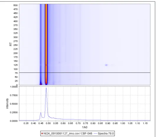
Figure 4.1.: Heatmap with detail view of a selected single spectrum. The heatmap consists of 500 single spectra which are pseudo coloured using a heatmap paint scale.

4.1.1. Normalisation and alignment

To align spectrometric data, sampling points have to be found which refer to identical substances and occur in every measurement. Align-ment methods for IMS technology benefit from the fact that the RIP (see Section 2.2) occurs in every measurement and that its intensity refers to the strength of the ionisation energy of an IMS.

1

/ k

₀

alignment

The first step in the alignment process is transforming the 1/ k₀ _axis

by moving the spectra until the RIP 1/ k₀ _{value matches the default}

position of 0.485. For this procedure, termed 1/ k₀ alignment_{, the}

po-sition of the RIP needs to be determined exactly. A spectrum subset needs to be selected which ensures that the maximum of the RIP is not influenced by analytes or disturbing effects. The probability for analytes to occur decreases over the retention time, because most of

(37)

4.1. Spectra pre-processing ₃₃

the molecules of a volatile gas sample have a small collision cross sec-tion and pass the MCC in a short amount of time. Therefore, the last 100 spectra of a measurement are used for the subset. The RIP is de-tected by finding the maximum of every spectrum of the subset and putting its 1/ k₀ _{value into a sorted list. Afterwards the median of this}

list delivers the 1/ k₀ _{position of the RIP. Due to the robustness of this}

procedure this can be done fully automatically without additional user input or parameter settings.

Intensity normalisation

The next step is a normalisation of the intensity axis to verify the com-parability between measurements. This is important especially when comparing data recorded by different devices. Therefore, the abso-lute values are transformed to values relative to the maximal available ionisation energy. Since the maximum of the RIP reflects the maximal available ionisation energy of one specific IMS, the maximal intensity of the subset formed for the 1/ k₀ _{alignment is chosen for}

normalisa-tion.

Retention time alignment

The chromatographic column is responsible for the pre-separation a-long the retention time axis and divides the sample into a number of single spectra. The time needed for analytes to pass the column de-pends on several factors such as temperature, pressure, and condition of the inner surface. Although much effort is put into keeping these fac-tors stable, small variations cause analytes to occur at slightly different retention time points. These so called retention time shifts_{need to be}

corrected to allow exact comparison between measurements and ana-lyte identification. The RIP can not be used as a reference here since it occurs in every spectrum. Furthermore no reference analyte is brought into the probe and no analyte could be found which occurs constant in every measurement. But experiments showed that there are ex-periment specific analytes which can be manually chosen to align the retention time axis. For example in cell culture probes (see Section 2.1.1) there are analytes which are caused by the medium and such caused by the cells. Since the aim of these experiments is to compare different cell cultures on the same medium or, vice versa, the same cell culture on different media, analytes c₁, . . . , c_n _{can be found that}

occur in every measurement. A retention time target RT T(c) _{for at}

least one of such constantly occurring analytes has to be chosen to find a retention time alignment factor (RT F) _{for each measurement.}

(38)

This is done by dividing the target position of an analyte RT T(c) _by

the actual position of an analyte in the measurement RTA(c)_, RT F=

RT T(c)

RTA(c) (4.1)

.

After scaling the retention time of every spectrum of a measurement with this factor, the retention time axis is called aligned _{and can be}

used for comparison and identification. If more constantly occurring analytes with differing retention times are available, this process can also be done more than once on specific retention time intervals, but experiments showed (see Chapter 6.3) that the correction using one analyte is sufficient for further analysis and using more analytes can lead to false deformations.

4.1.2. Baseline correction and RIP compensation

While the fact that the RIP occurs in every spectrum is a great advan-tage for 1/ k₀ _{alignment and intensity normalisation, it is also}

obstruc-tive for further analysis and visualisation. It dominates every measure-ment but contains nearly no relevant information about the analytes of a sample.

Figure 4.2.: _{Influence of the RIP compensation filter on an IMS heatmap.}

Left: Raw measurement; Right: Compensated RIP

One major problem is the so calledRIP-tailing_{, the part of every}

spec-trum from 0.50 to 0.80 1/ k₀ _{where the RIP increases the baseline of a}

whole spectrum with a diminishing value. This causes a difficult sep-aration of peaks from noise and problems when altering the colour

(39)

4.1. Spectra pre-processing ₃₅

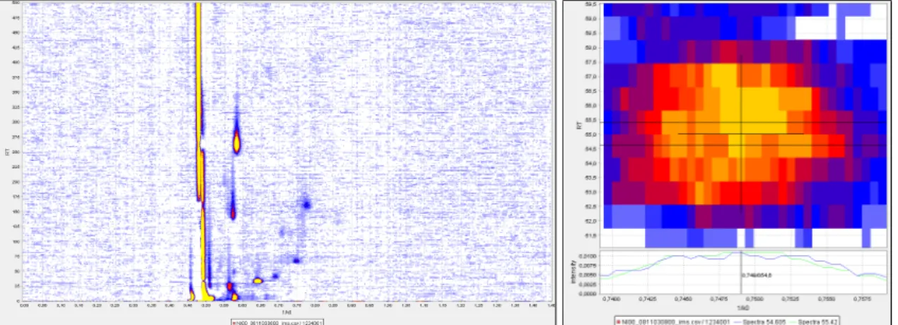
Figure 4.3.:Two heatmap images of a measurement with compensated RIPwithout_{applying any filter methods. The left part shows} a complete measurement while the right part shows a de-tailed zoomed view of one single peak.

space of a heatmap for better peak visualisation as shown in the left part of Figure 4.2. To compensate for this effect, the RIP needs to be determined and subtracted from every spectrum. Therefore, all values with the same 1/ k₀ _{are brought into an ascendingly sorted list and the}

25% quantile for every 1/ k₀ _{is selected. These values form the} low quantile spectrum _{and represent the part of a measurement which all}

spectra have in common. The quantiles are chosen because the the-oretically necessary minimum of each 1/ k₀ _{is zero in most cases due}

to noise and thus unusable for this task. Subtracting the low quantile spectrum removes the RIP together with its tailing and also corrects the baseline of every spectrum.

4.1.3. Filtering

Different filter operations are necessary to remove noise from the mea-surement and thus improve the quality of the data for further process-ing steps and visualisation. To determine the quality of filter operations and to verify that the position and quantification of analytes is not al-tered, control criteria are chosen. The first criterion is the area from 0.1 to 0.4 1/ k₀ _{where no analytes can occur. The second criterion is}

the position and intensity of peaks in the measurement. An optimal filter reduces the noise of the first area while keeping the values of the peaks constant.

Two different filters showed an improvement of the data under these conditions and were therefore composed as a default filter pipeline for IMS data. The filter pipeline first uses a median filter and afterwards a Gaussian filter to remove noise from the data. An example of the

(40)

performance of this filter pipeline is given here, the detailed examples to show the result of the single filters are available in the Appendix.

The median filter approach was chosen to eliminate single noise frag-ments from the data. Basically it replaces every value of the measure-ment with the median of the neighbour values. As Figure 4.3 shows, the number of values of a measurement which do not form peak struc-tures and thus contain no information needed for further analysis is high.

ˆ

ƒ(, y) =medn

(s,t)_∈Sy

{g(s, t)_}. _(4.2)

Since the time needed to process and visualise measurements de-pends on the number of datapoints to handle, reducing them without losing information is advantageous. In the pipeline the filter uses a five times five area as neighbour values, resulting in a list of 25 values to determine the median. The median filter is applied first to elimi-nate single isolated values which otherwise would be blurred and thus turned into several values by following filters.

The Gaussian filter was applied to smooth the remaining values and preprocess them for the peak detection and visualisation methods. It is termed Gaussian filter because the resulting impulse response is a Gaussian function. G(, y) = _p 1 2πσ2 e− 2₊y2 2σ2 (4.3)

Where Sigma_{is the standard deviation of the Gaussian distribution.} s(, y) = X

(,j)_∈M

ƒ(+, y+j)h(, j) _(4.4)

Equation 4.3 can be used to create a gaussian filter mask G _and

Equation 4.4 shows how to convolute a given mask h _{with the original}

heatmap image f_.

In the filter pipeline it is used with the smallest possible two dimen-sional mask size three times three, to prevent a distortion of the later determined peak intensities.

The effect of the filter pipeline on MCC-IMS data is shown in Figures 4.3 and 4.4.

4.2. Peak detection

Peak detection is the process of generating a list of detected peaks out of the intensity matrix of every measurement. This is needed for two main reasons. Firstly it is much faster to process a list of peaks than to

(41)

4.2. Peak detection ₃₇

Figure 4.4.:Two heatmap images of a measurement with compensated RIP after applying the filter pipeline. The left part shows a complete measurement while the right part shows a de-tailed zoomed view of one single peak.

process the complete data matrix of an MCC-IMS measurement. Sec-ondly, the alignment of the axis is not accurate down to the level of single data points. The position of the maxima of identical analytes can vary through different measurements. Although these variations are usually low, it eliminates the possibility of direct datapoint compar-ison through different measurements.

A suitable method to detect peaks in this kind of data is the water shed transformation_{, which was successfully applied by Wegner et al}.

for spot detection in two-dimensional gel electrophoresis images [40]. They illustrate the idea of this transformation by thinking of the data as a topological permeable map which is submerged into an imagi-nary water basin. In case of MCC-IMS data the map has to be flipped that the peaks touch the water surface first. The water that enters the map forms a pool for every elevation and with the rising water level more pools emerge which are called regions_{. The borders where two}

regions touch each other are termed water sheds_{. This concept is}

im-plemented by putting all values of a measurement into a list, descend-ingly sorted by their intensities. In addition a segmentation matrix of the same size is initialised. For each item the adjacent fields of the segmentation matrix are checked. One of three actions is performed afterwards, depending on the number of regions to which these adja-cent fields belong:

a) If none of the adjacent fields are defined inside the segmentation matrix then a new region is created. An identifier for this region is defined at the respective position and the point is added to this region.

(42)

b) If one of the adjacent fields already belongs to this region, then the current point is added to a region and marked in the segmen-tation matrix.

c) If adjacent fields of an entry belong to different regions, the coor-dinates are marked as water shed in the segmentation matrix. The result of this method is a list of regions which are surrounded by water sheds. The maximum of each region is used to determine the maximum of a peak and all members of the region are used to determine the volume.

After the peak detection all detected and quantified analytes of one measurement are available as a list of peaks. The 1/ k₀ _{and RT}

param-eters of a peak are termed peak position _{and the peak maximum is}

termed peak intensity_.

4.3. Data analysis

After the successful peak detection, areas need to be defined to com-pare peaks from different measurements. Those areas consist of a name, a RT and a 1/ k₀ _{parameter to determine its position, and two}

values to define the tolerance values for each parameter. Those val-ues can either be taken from a list of known substances which were already determined in previous MCC-IMS measurements or by setting up a new area with a user interface.

Subsequently a dataset can be regarded as a table with one line for each measurement and one column for each substance as proposed in Figure 3.1 in the Requirements chapter. The main IMS data analysis questions which occur in the biological, chemical and medical context are then settled in the field of correlation and classification.

Correlation analysis is always needed when additional experimen-tal parameters are known and dependencies between these parame-ters and occurring substances or dependencies between multiple sub-stances should be detected.

Classification analysis enables the partition of measurements into different groups. This can be done by unsupervised techniques to de-tect similarities between measurements without any prior knowledge or supervised when the groups are already known.

For these kind of data and questions a vast number of methods is available. Commonly used techniques like support vector machines

and artificial neural networks _{are able to perform supervised}

classi-fication techniques, but the explanation of the results is difficult to understand, since they contain a black box model. This means that

(43)

4.3. Data analysis ₃₉

there is no information available how important a specific analyte is for the classification result or which analytes are characteristic for a class. Since this information is necessary or even the aim of many IMS experiments, especially in the breath diagnostics field, analysis methods which contain any kind of black box are not suited to chal-lenge this task. Unsupervised techniques like clustering methods are as well difficult to apply because the similarity between the different measurements is usually high. Many regions of the measurements are often similar and substances which are important for a specific exper-iment need to be determined. Therefore, approaches to analyse IMS data based on peak intensities while retaining the information about the peak characteristics and their related classes are described in the following.

4.3.1. Defining intensity thresholds

The basic criteria for a data analysis of spectrometric data are the de-tected and quantified peaks. One key question in the IMS data analysis context is if there exist one or more peaks whose intensities corre-spond to a previously defined class of measurements. Such relation between classes and intensities can be used to predict classes of so far unknown datasets, and gives information which peaks and thus an-alytes are possibly produced or caused by measurements of one class. This question can also be formulated as the search for an intensity threshold which allows the separation of a dataset into the previously defined classes.

The ideal case would be that one peak occurs on exactly the same position in every measurement of one class and never in any other. Since the position and intensity of peaks can be influenced by many different factors like pressure, temperature, air flow, and assigned classes can be inaccurate the chance that such peaks exist and can be found is low.

A more probable case is shown in Figure 4.5 where a relation be-tween peak and class is visible although no clear separation is possi-ble. Tolerance values have to be defined to determine the maximal al-lowed difference between the identified position of an analyte and the detected peak positions. To enable the partitioning into two classes, an intensity threshold has to be defined. All measurements with a spe-cific peak equal or above this threshold are regarded as members of the first class, all other as members of the second class. An intensity threshold is considered as appropriate when the number of wrongly assigned classes through this procedure, compared to the previously defined classes, is low.

(44)

Figure 4.5.: _{The left part shows the peak intensities of 4-Heptanone in}

two different classes. A relation between classes and peak intensity seems probable. The right part shows the distri-bution of the peak positions. While most of the peaks are very close to the proposed position of 4-Heptanone in the centre, some differ within defined tolerance boundaries

As an experiment typically consist of a high number of measure-ments and detected peaks, a manual analysis is time consuming in the best case and impossible in the worst case. An optimisation of the tolerance values can increase the chance of detecting intensity thresh-olds and increase the quality of an analysis. These findings lead to the development of an automatic procedure to rate peaks based on their relation to a class and determine their optimal boundaries.

4.3.2. Detecting optimal intensity thresholds

To detect appropriate intensity thresholds, the high number of possi-ble peaks and thresholds need to be rated by an automatic process. Therefore a scoring procedure was developed to determine the quality of all possible thresholds.

To determine if two peaks from different measurements belong to an identical analyte, two initial tolerance values are defined, one for retention time and one for 1/ k₀ _{. For the retention time tolerance, 10%}

of the peak’s retention time plus a fix value of 5 seconds is chosen. The percentaged value fits the tolerance to flow factors which can vary between different pre-separation columns while the fix value covers position shifts caused by noise. Since the 1/ k₀ _{values of peaks are}

known to be very constant, the tolerance has to cover only small shifts caused by noise, leading to a tolerance value of 0.015 1/ k₀ _.

All detected peaks from all measurements are inserted into a list, sorted by their retention time. For every peak in the list, a subset is created which contains all peaks with a retention time difference smaller than or equal to the tolerance. This is done by first moving down in the list starting at the peak’s original RT until the tolerance or

(45)

4.3. Data analysis ₄₁

Figure 4.6.:_{Peak intensities of 4-Heptanone displayed as bars and}

la-beld with previously known classes A and B. The inten-sity is shown on the left axis. The separation accuracy graph shows the percentaged number of correctly assigned classes when assigning all measurements containing peaks with an intensity equal to or higher than this value to class A and all others to class B. The right axis shows this per-centage.

the end of the list is reached, afterwards moving up in the same man-ner. From this subset, all elements are removed where 1/ k₀ _distance

to the peak exceeds the 1/ k₀ _{tolerance. Peaks from this subset which}

belong to an identical measurement are a strong evidence that the tol-erance values are too high and should be altered to prevent this effect. The peak which is closest to the starting peak is kept while the others are moved to a duplication list to create optimised tolerance values.

Using this method, a subset of peaks is assigned to every detected peak. To rate them, the peaks of every subset are sorted in descending order by their intensity. Now a score is assigned to every possible intensity threshold by counting the number of correct threshold based class assignments compared to the known classes to find appropriate intensity thresholds. Figure 4.6 shows an example where one of two possible optimal scores is achieved when setting the threshold to an intensity of 0.0083 resulting in separation between samples nr. 30 and nr. 31. Separating at this point assigns 44 of the 51 measurements to the correct class which equates approximately 86.3 percent. This score gives information about the quality when assigning all measurements that contain this peak with an intensity higher or equal to a first class and below this intensity to a second class.

(46)

Figure 4.7.: Automatic centering effect of the scoring procedure. The black crosses mark the positions of the peaks. The purple cross is the center used to form the subset shown in the left diagram, the green cross is the center for the subset shown in the right diagram. The maximal achieved score is written in each diagram, showing that the subset formed by the peak in case 2 is a better separation criterion than the subset formed by the peak in case 1.

Sorting the list of all peaks descending by their assigned accuracy score orders them by their performance when using them as a sepa-ration criteria. Comparing every peak to every other peak inside the tolerance boundaries leads to multiple entries which have a very simi-lar position and thus refer to the same analyte. Although they have a very similar position, some of them differ in their assigned score which can be seen in Figure 4.7. Peaks which have a higher distance to the centre of their possible group typically achieve a lower accuracy score. This is because a peak in a measurement that does not fit into the tolerance boundaries is considered as not present and marked with an intensity value of zero. Under the assumption that these excluded peaks are approximately equally distributed in the two classes, this results in an automatic detection of an optimal score centre.

4.4. Visualisation and exploration

A visual representation of the data which displays all information about an experiment and allows detailed examination of different areas is one of the most important parts of an IMS analysis. The pre-processed and aligned spectra need to be displayed together with detected peaks

(47)

4.4. Visualisation and exploration ₄₃

and identified analytes and defined tolerance boundaries. This is nec-essary for verification of quality and results of the measurements as well as quality of the performed pre-processing, alignment, peak de-tection an intensity thresholding methods. Interactive visualisation also allows to identify important analytes and areas of the measure-ment as well as general interpretations.

Since all analysis of IMS data are based on parallel examinations of many measurements, techniques for parallel visualisations are neces-sary. The key informations every IMS measurement contains are the concentrations of the analytes. These are described through the pa-rameters of the detected peaks. Visualising and comparing a high number of these parameters gives information about the characteris-tics of analytes and thus enables interpretation and understanding of the data.

4.4.1. Heatmap visualisation

The normalised spectra are composed to an intensity matrix and dis-played as a heatmap. A heatmap is a visualisation technique where three parameters of an arbitrary number of data points can be dis-played in parallel. Two parameters describe the position of each pixel on a two dimensional map, the third parameter is encoded by the colour of the pixel.

Figure 4.8.:_{Colour space used to generate the heatmap visualisation.}

The position of each IMS data point on this map is determined by its 1/ k₀ _{value in horizontal position along the X-axis and its RT value in}

vertical position along the Y-axis. The intensity is mapped to a colour space shown in Figure 4.8. Intensity values which are lower or equal zero after the pprocessing are excluded from the visualisation to re-duce the time needed for generation and thus enable a fast browsing through a high number of measurements. The emerging free areas in the heatmap are use to paint grid lines for precise determination of 1/ k₀ _{and RT values of analytes on the axis. The colour space is}

(48)

Figure 4.9.: Visualisation of the intensity distribution of one single peak. The bar chart and the boxplot on the left show the distri-bution of the selected analyte on the right in 4 different classes. The intensity of the selected analyte is higher in classes B and D than in classes A and C. The lower part of the right picture shows one selected spectrum, marked with a black line in the heatmap.

designed to map values between zero and one to a colour range start-ing with white gostart-ing on to blue, red, and endstart-ing with yellow for high intensities.

4.4.2. Peak intensity visualisation

After a successful peak detection and the definition of tolerance bound-aries, all intensity values of peaks which satisfy the constraints can be visualised in different ways. Since many experiments aim at the c