News text generation with adversarial deep learning

News text generation with

adversarial deep learning

Filip Månsson, Fredrik Månsson

MASTER’S THESIS | LUND UNIVERSITY 2017

Department of Computer Science

Faculty of Engineering LTH

News text generation with adversarial deep

learning

Filip Månsson

Fredrik Månsson

September 6, 2017

Master’s thesis work carried out at Sony Mobile Communications AB.

Supervisors: Håkan Jonsson,[email protected] Pierre Nugues,[email protected]

Abstract

In this work we carry out a thorough analysis of applying a specific field within machine learning calledgenerative adversarial networks, to the art of natu-ral language generation; more specifically we generate news text articles in an automated fashion. To do this, we experimented with a few different architec-tures and representations of text, evaluated the results and used the information retrieved from the results, to create a model that should give the best result. For evaluation, we used perplexity and human evaluation. We also looked at the token distribution to see which model captures the texts most successfully. We show that it is possible to use generative adversarial networks to gen-erate sequences of tokens that resemble natural language, but this does not yet reach the quality of human-written text. Further hyperparameter tuning and using a narrower-subjected corpus could improve the output.

Keywords: Machine learning, generative adversarial learning, GAN, natural lan-guage generation

Acknowledgements

We would like to thank both of our supervisors for helping us with this project and taking the time and effort to answer our questions as well as providing us with valuable feedback. We also want to send our regards to our parents and siblings for their support throughout our lives.

Contents

2.2.1 Convolutional neural networks . . . 12

2.2.2 Recurrent neural networks . . . 12

2.2.3 Long short term memory . . . 13

2.2.4 Residual learning . . . 13

2.3 Generative Adversarial Networks . . . 13

2.3.1 Generator . . . 15 2.3.2 Discriminator . . . 15 2.3.3 Cost function . . . 15 2.3.4 Algorithm . . . 15 2.3.5 Known issues . . . 16 2.4 Wasserstein-GAN . . . 16 2.4.1 Generator . . . 17 2.4.2 Critic . . . 17 2.4.3 Cost function . . . 17 2.4.4 Algorithm . . . 18 2.4.5 Known issues . . . 18 2.5 Improved Wasserstein-GAN . . . 19 2.5.1 Cost function . . . 19 2.5.2 Algorithm . . . 20 2.5.3 Known issues . . . 20 2.6 Text Representation . . . 20

3 Approach 23 3.1 Overall Approach . . . 23 3.2 Setup . . . 23 3.2.1 Corpus . . . 23 3.2.2 Training . . . 24 3.3 Models . . . 25 3.3.1 Baseline . . . 25 3.3.2 GAN model . . . 25 3.3.3 WGAN models . . . 25 3.3.4 Motivation of approach . . . 29 4 Evaluation 31 4.1 Metrics Used . . . 31 4.1.1 Perplexity . . . 31 4.1.2 Human evaluation . . . 32 4.2 Results . . . 32

4.2.1 Results using characters . . . 33

4.2.2 Results using words . . . 33

4.2.3 Generated text . . . 43 4.3 Final Model . . . 47 4.4 Human Evaluation . . . 50 4.5 Discussion . . . 51 5 Conclusions 55 5.1 Conclusions . . . 55 5.2 Future Work . . . 56

Appendix A Generated articles 63

Chapter 1

Introduction

This chapter gives a brief overview of the topic at hand and the problem formulation of the thesis as well as related work. We also provide a short description of the contributions.

1.1

Overview

Recently there have been an increasing number of reports about the impact that fake news has on the world, not exclusively constrained to elections but also to other influential areas of the global market such as the stock market (Rapoza, 2017). The source of the fake news can be driven by the purpose of actually affecting an outcome or simply to increase the living standard by making a quick and simple profit of them (Kirby, 2016). What these sources have in common is that there is a human being behind the texts.

Over the past few years machine generated texts become more and more common within all from news articles (Eidnes, 2015) and scientific reports to plays inspired by Shakespeare (Karpathy, 2015). Today there are several different methods and techniques available for producing texts of various types and qualities. As computation power grew with time, so did the complexity of the models capturing the languages. Many of the more successful models are based on deep learning and neural networks (Karpathy, 2015). A more recent model not primarily used for text generation is the generative adversarial network, (GAN).

The main idea behind GAN (Goodfellow, 2017) is that instead of training one network you train two and you train them against each other as in the mini-max game. One of the players in the game is called the generator, whose purpose is to generate samples that resemble those drawn from the training data. The other player is thediscriminator, re-sponsible for classifying samples as real or generated. The generator is trained to produce samples that deceive the discriminator, while the discriminator is trained on the classified samples as in traditional supervised learning.

1.2

Problem Definition

The goal of this thesis is to implement and make use of GANs for generation of news articles. The primary objective is to make the articles readable with less emphasis on truthfulness. Therein we will also get an understanding of the potential within automatic text generation and possibly also generate a corpus containing fake articles as an aid for creating methods of classification. We will look into how text has been generated previ-ously using machine learning methods and then try to incorporate the learned information into the attempt of utilizing a GAN for the purpose of generating news articles. We will at-tempt to use a few different architectures, evaluate these, and finally use the insights made to create a better model.

We are specifically going to look at the original GAN andWasserstein-GAN(WGAN) for text generation. We will train models with different settings and architectures and evaluate them using perplexity and human evaluation. We will also look at the distributions of tokens within the texts.

1.3

Related Work

The topic of text generation is gaining more attraction and research regarding this area is on the rise. The following text piece discusses research that is related to our work.

Text generation has been done by different approaches such as a sequence to sequence model by Sutskever et al. (2014) where they translated English texts to French by using two

long short term memory(LSTM) networks: one encoder and one decoder. The nature of this model also allowed for a varying input length as the output from the encoder is always mapped to a vector of a fixed size. The result of the implementation showed comparable to a referencestatistical machine translation system(SMT). This good result was partly achieved due to the fact that they were using LSTM cells, cells that are specifically designed to remember long term dependencies. The authors also stated that they achieved a better result by reverting the input to the translator.

When it comes to generating realistic images GANs have proven to be successful. However, regarding the task of generating text or any kind of task which involves text as input or output, the use of GANs has not yet been as satisfactory. Many of the issues concern the representation of text as a continuous space according to Goodfellow (2017). GANs have only recently been applied to text generation; for instance Li et al. (2017) has applied them to dialogue generation using reinforce algorithms. The authors use a GAN and compares the performance with more common methods of dialogue generation. The paper also introduces some useful tricks such as teacher enforced training to guide the generator towards the right path. This is done during the generation process of the training, by having a “teacher” intervene and force the generator to output the correct response.

A known problem with generating discrete outputs such as words is the inability to back-propagate useful information from the discriminator to the generator. Kusner and Hernández-Lobato (2016) overcome this problem by using the Gumbel-softmax distribu-tion and managed to generate discrete sequences of elements.

Another approach was investigated by Zhang et al. (2016), where they use an LSTM network as generator and anconvolutional neural network(CNN) network as

discrimi-1.4 Contributions

nator. The LSTM network worked as an encoder, mapping from an encoded feature vector (word embeddings) to the succeeding word; in this case the output is in the form of one-hot encoding i.e. a binary vector of the same size as the vocabulary and the only legal combination of values are those with a single one and all others are zeroes. So a word will be represented by a vector of zeros except for at the specific words index, where there is a one. A sentence was constructed by always choosing the word with the highest proba-bility given the previous word/vector and by applying anargmaxfunction to the output of the generator. This was repeated until the generator reached the end of a sentence (a special token). The discriminator is pretrained by being fed real sentences and sentences with swapped word order. By doing so it should learn the structure of sentences. The problem with discrete outputs was then solved using an approximated discretization by using asoftmaxfunction followed by anargmaxoperation. By feeding generated sen-tences and real sensen-tences to the discriminator, they carried out training in an adversarial way, where a form of feature matching was used instead of the original objective function proposed by Goodfellow et al. (2014).

1.4

Contributions

We hope the results produced by this thesis will help Sony Mobile Communications in the evaluation of the potential of GANs. The goal is to contribute to the research on how to represent words and how to use GANs to generate text. The thesis will hopefully also aid with the creation of a corpus useful when investigating methods for detection of fake news and thereby prevent some spread of misinformation.

From what we can see we are the first to have our model output embeddings directly instead of using a one-hot encoding. We are also among the first to use the WGAN structure for generating text.

Chapter 2

Background

This chapter covers the background of text generation and more about neural networks as well as deep learning. More information is also provided concerning generative adversarial networks of different flavors.

2.1

Text Generation

Natural language generation (NLG) is the science of “linguistic manipulating of data” and “NLG manipulates (linguistically) deeper information to produce shallower information” (Evans et al., 2002). As a result of this definition, it is not enough to simply parse the data or keep the same level of information (as for instance creating a summary or translating a text), but by using the data to produce new information.

There exists several techniques for NLG including rule-based, statistical and data-driven. Rule-based models rely on hand-written specialized rules for generation. Included in the rule-based models are also template-based where the models make use of predefined phrases or grammar. The problem with these are that they often require many rules to be crafted and the resulting model will often be restricted to a small specialized domain as well as a small vocabulary. This in turn means that the model may perform very well but it lacks flexibility (Manishina et al., 2016).

Statistical models (usually some combination of N-gram models) are based on counts retrieved from the training data. The models allows for explicit modeling of the context and joint probabilities. The issue with these models arise because they are limited to what they see and their assumption of independence. This results in that these models can’t capture any long term dependencies (not longer thanN).

1 0 1 0

Kernel

Data

Feature map

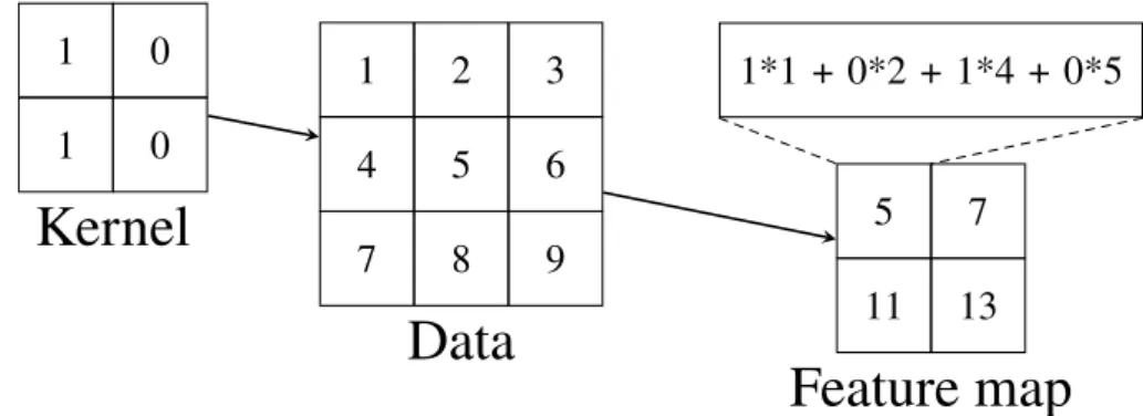
Figure 2.1: Illustrating a simple 2D convolution with a kernel size of 2x2 and a stride of 1. Here we use the “valid” technique where we restrict the output to only consist of points where the kernel completely fits within the input.

2.2

Neural Networks

Deep learning uses neural networks (or artificial neural networks) as building blocks. This name comes from the idea that the models used in deep learning has been engineered to mimic or take inspiration from the brain. In the early beginning of neural networks, as early as the 1940s, they were using simple linear models to classify the inputs as belonging to one of two classes. Today a lot of the trained models rely on algorithms that were developed by the early researchers but could not be applied as the computation costs where too high. Neural nets have also had an recent upswing as it has become easier to find large data sets, which in turn means that it requires less tuning of the nets, (Goodfellow et al., 2016, p. 13-20).

2.2.1

Convolutional neural networks

Convolutional neural networks (CNN), are a type of network that is applied on matrix or grid-like data. The first word in the name, i.e. convolution, reveals that the main operation in this type of network is the convolution operation. You can think of a convolutional op-eration as taking the weighted average of several data points. When dealing with chunks of data in matrix form this can be seen as the dot product. You place the aforementioned weights in a matrix called the kernel of the wanted size. Usually the kernel is much smaller than the matrix containing the data and therefore you will need to stride, meaning that you slide the kernel over the data matrix. The final result or the output of the convolutional op-eration is called a feature map. See Figure 2.1 for a visual demonstration of a convolution, (Goodfellow et al., 2016, p. 330-334).

2.2.2

Recurrent neural networks

Recurrent neural networks (RNN) is another flavor of neural networks. Unlike the CNN that specialized in processing grid-like data structures the RNN model was created to man-age sequential data. Recurrent neural networks make use of parameter sharing across the

2.3 Generative Adversarial Networks

model layers. The sharing of parameters makes it possible to generalize and use the same weights over different positions in time. This means that it doesn’t matter whether for in-stance a word is at the first position of the sentence or in the last, the model will treat it the same way, (Goodfellow et al., 2016, p. 373-374).

2.2.3

Long short term memory

Normally RNNs are capable of using context information i.e. predicting the next word given the previous, but this becomes harder as the distance between the dependencies within the sequences grows. For instance given the sequence “My name” even the standard RNN model should be able to simple predict that the next word is “is”. Consider the sequence “Last summer I went to Denmark for vacation. It was ... I have decided that next year I will return to” we want the model to predict “Denmark” but it is not easy for the model to remember the dependency. Long short term memory network (hereon referred to as LSTM) is a variant of RNN developed to solve this issue. The key concept to LSTMs is the cell state, a memory keeping track of vital information that the cell has seen. This state can for instance contain information about the subject of the sentence as is it a thing or a person and based on that use the correct pronoun. In each interaction with a LSTM cell, the internal workings decides what to do with the state, whether to remove or add information to it, (Olah, 2015).

2.2.4

Residual learning

A more recent technique introduced into the deep learning community is the use of residual learning (goes also under the name residual block or resblock). The main purpose behind residual learning is to remove the degradation of training accuracy introduced by the depth of a model. The solution is to use a shortcut from the input of the block to the output. This has shown great empirical results, (He et al., 2015).

2.3

Generative Adversarial Networks

Generative adversarial networks (GANs) were first introduced by Goodfellow et al. (2014) and have become very popular. Despite its rather new entry to the family of machine learning techniques, it has shown great results when applied to image synthesizing.

Generative adversarial networks belong to the family of generative models. Given a set of training data from a distribution, GAN models will learn a distribution representing an estimate of the original data distribution. The model can either represent an actual dis-tribution or it can generate samples from one. Often it is the latter, generation of samples, which is more common.

Training models often mean that you need to have a data set with labels for all data. However generative models can be trained with a data set containing a mix of both labeled and unlabeled data, removing an otherwise limitation caused by some lack of information (Goodfellow, 2017).

Conventional training in machine learning is based on minimizing the differences, usu-ally MSE (Mean squared error), between the output and the target. This is clearly not

pos-Real samples Generator

Real and gen-erated samples

Discriminator

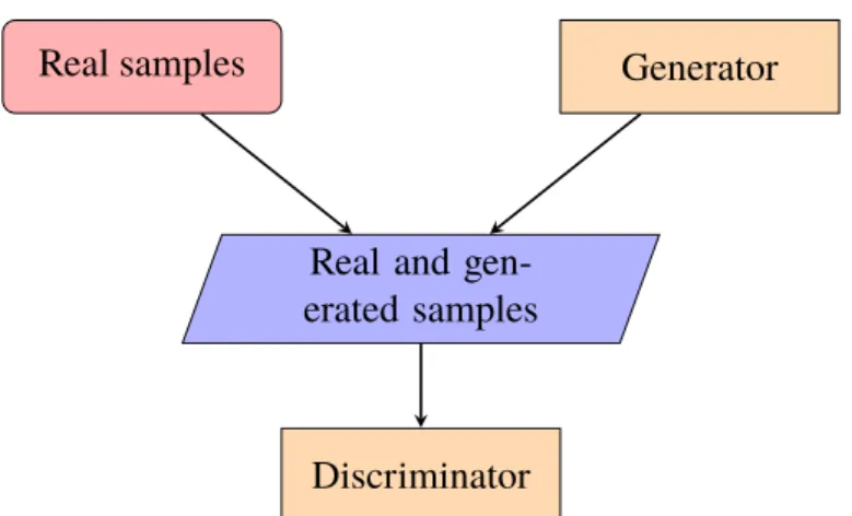
Figure 2.2: Illustrating the overall structure of the GAN

sible when there might be multiple targets which brings us to another advantage of GANs: the property to cope with outputs which are multi-modal, i.e. each input may correspond to multiple outputs, which are all correct. This was illustrated in Lotter et al. (2015) where the task was to predict the next frame given previous frames in a video. In the video, a human looking face was rotating at random speed. There are therefore multiple frames that all could be correct. By using the approach of GANs, the predicted frame was clearer suggesting it had chosen a single frame and not an average of frames as was the case when using a MSE loss.

If we instead look at what kind of data text is, how could this multimodal property show? We know for instance that there are multiple ways of describing an object. Consider for instance the task of describing a car. The car has four wheels, a steering wheel, windows and so on. But it also has a color. We can change the description of the car by giving it another color. The descriptions are no longer the same since the colors are different but they are all correct since they all describe the same object, a car.

The ability to generate samples originating from a distribution means that we do not actually need to explicitly learn a complete distribution. This is especially important when the distribution is high dimensional or for some other reason hard to represent or learn. Representing all possible articles would require a hyperspace of infinite dimension. Rep-resenting all English words or a fraction of them is tractable but then you need to learn what words should be in an article, in what order, how long should the article be and so on in order to generate new ones.

Generative adversarial networks consist of two models, a generator and a discrimina-tor. By having samples of data drawn from a distribution representing our target distri-bution, the generator’s purpose is then to use noise as input, often a uniform distridistri-bution, and generate samples that look like they were drawn from the same distribution as the data samples. The discriminator is fed with data samples from the “real” distribution and samples that are fake, generated by the generator, and is then asked to predict which ones are real and which ones are fake. The output from the discriminator is then propagated to the generator so as to update, improve and generate more realistic samples. You can think of it this way: the generator acts as a criminal producing counterfeit money and the discriminator as the police trying to discriminate fake money from real. For an overview of the network see Figure 2.2.

2.3 Generative Adversarial Networks

2.3.1

Generator

The generator is defined as a functionGthat is differentiable with respect to its parameters

θgand inputz. zis to be considered as noise drawn from a distributionPz, e.g. some Gaus-sian (normal) distribution. The generator will then mapzto samplesG(z) corresponding to a sample drawn from the generator’s distributionPgwhich will hopefully after training be the same as the true data distribution Pdata. The mapped samples G(z) are fed to the discriminator and the generator is then trained to fool the discriminator by having it give high probabilities to the generated samples.

2.3.2

Discriminator

The discriminatorDis just like the generator differentiable with respect to its parameters

θdand inputxandG(z), wherexis real data samples drawn from thePdatadistribution. The discriminator then outputs a value representing the probability of the sample belonging to the real data distribution Pdata. The discriminator will then be trained, in a supervised setting, to give a high probability to real data samples and a low to samples generated by the generator.

2.3.3

Cost function

In a more mathematical perspective, the generator and discriminator cost functions are related by Equation 2.1. min G maxD ExvPdata(x) logD(x)+ EzvPz(z) log(1−D(G(z))) ! (2.1) Where_ExvPdata(x)andEzvPz(z)are the expected values of thePdata andPzdistributions. Optimizing Equation 2.1 with respect to the discriminator will result in minimizing the Jensen-Shannon divergence betweenPdataand thePgdistribution, see Equation 2.2.

JS(Pdata,Pg)= DK L Pdata Pdata +Pg 2 ! +DK L Pg Pdata+Pg 2 ! (2.2) whereDK Lis the Kullback-Leibler divergence:

DK L(Pdata(x)||Pg(x))=

Z ∞

−∞

Pdata(x)

Pg(x) Pdata(x)dx

Since the generator’s cost function is dependent on the discriminator’s parametersθd, and the discriminator’s cost function is dependent on the generator’s parametersθg, the solution will also be equivalent to a Nash equilibrium which will be where the generator’s cost function is minimized with respect toθgand the discriminator’s cost function is minimized with respect toθd, (Goodfellow, 2017).

2.3.4

Algorithm

Algorithm 1 describes how the training procedure is carried out in generative adversarial networks.

Algorithm 1Implementation of GAN

1: procedureGAN

2: fornumber of iterationsdo

3: fornumber of steps to runDdo

4: z← minibatch of m samples from Pz(z).

5: x← minibatch of m samples from Pdata(x).

6: Update D by maximizing: 7: D← ∇θd 1 m m P i=1 logD(x(i))+ log(1−D(G(z(i)))) 8: z←minibatch of m samples from Pz(z).

9: Update G by minimizing: 10: G ← ∇_θg1 m m P i=1 log(1−D(G(z(i)₎₎₎

2.3.5

Known issues

We have already mentioned a vital problem with GANs and that is their inability to gener-ate discrete outputs such as words. The reason behind this is that the generator needs to be differentiable and thus can only have continuous data as input (Goodfellow et al., 2014).

When convergence is reached the generator should produce samples similar to those drawn from Pdata. However, GANs consist of two networks trained by maximizing and minimizing the cost function depicted in Equation 2.1. This is unfortunate since updating one of the networks may be the same as moving the other network in the opposite direction, away from convergence and in worst case the Nash equilibrium will never be reached. The two networks will then get stuck and the outputs only oscillate between the same points.

One of the problems originating from non-convergence ismode collapseor sometimes referred as thehelvetica scenario. Mode collapse occurs when the generator maps differ-ent samples from Pzto the same point x. As mentioned by Goodfellow et al. (2014) the generator must not be trained too much, effectively overpowering the discriminator, since an optimal generator is the Dirac delta functionδ(x) where xare points the discriminator give high probabilities. This will of course result in a reduction ofPg approximation of Pdata. There are also problems concerning the power or capacity of the discriminator and the generator. If the discriminator is very confident and can sort out real and generated samples with high accuracy, the gradients backpropagated to the generator will vanish, meaning the generator will not improve any further. This scenario may happen any time, especially in the very beginning of training since the generator will not produce any real-istic samples at that time, (Goodfellow, 2017).

2.4

Wasserstein-GAN

Since the original paper about GANs was published there has been efforts to improve GANs and remove some of the known problems (mode collapse, stability). Wasserstein-GAN (WWasserstein-GAN) is one of them and was introduced by Arjovsky et al. (2017). They investi-gated how to best measure the divergence or distance between two distributions since this will largely affect the convergence. If the measure is weak, it will be easier to converge to

2.4 Wasserstein-GAN

the real distribution. The distance measure that was used by Arjovsky et al. (2017) is the Mover distance or Wasserstein distance. An illustrative way to look at the Earth-Mover distance is to think about it as a measurement of the cost for moving earth from one pile to another (the amount of earth times the distance the earth is moved), hence the name.

After running a set of experiments they concluded that most of the problems such as mode collapse and vanishing gradients never appeared. They also showed properties of the WGAN being more stable and not as dependent of the choice of hyperparameters. In addition the loss of the models related well to the quality of the output.

In order to emphasize what has been improved from the original GAN we will now explain the differences in more detail.

2.4.1

Generator

There is no difference between the generator compared to the original GAN, it still needs to be a functionGthat is differentiable with respect to its parametersθgand inputz, where zis data drawn from distributionPz. The only difference is the feedback it will get from the discriminator: it will now be a simple difference between the real and generated samples and not a difference between the probabilities. The generator will then fool the discrimi-nator by reducing the difference between real and generated data.

2.4.2

Critic

The purpose of the discriminator will no longer be to discriminate between real and gen-erated samples which is why it is now called critic. The critic will now only output the difference between two samples and will therefore be trained to give a large difference between the two samples. The criticC also needs to be differentiable with respect to its parametersθc and inputxandG(x), wherexis drawn fromPdata.

2.4.3

Cost function

The cost function for WGANs will use the Wasserstein distance instead of Jensen-Shannon as for GANs. The Wasserstein distance which we from now on will call Earth-Mover distance (EM) is given by Equation 2.3.

EM(Pdata,Pg)= inf γ∈Q₍ Pdata,Pg)E(x,y)vγ kx−yk (2.3) WhereQ

(Pdata,Pg) is the joint distributionγ, withPdataandPgas marginals.

The EM-distance in this shape will be difficult to calculate (Arjovsky et al., 2017). Arjovsky et al. overcame this by using the Kantorovich-Rubinstein duality which resulted in the cost function given in Equation 2.4.

min G maxC∈L ExvPdata(x) C(x)₋ EzvPG(z)C(G(z)) ! ,L∈1-Lipschitz functions (2.4)

Since we are now using the Earth-Mover distance there will be another constraint on the critic in Equation 2.4: the critic also needs to be 1-Lipschitz, i.e. a function that has gradients with a norm equal to one or less, which was solved by clipping the weights of the critic.

Optimizing Equation 2.4 with respect to the critic will result in minimizing the Earth-Mover distance betweenPdata andPg.

2.4.4

Algorithm

Algorithm 2 describes how the training procedure is carried out in Wasserstein-GAN as implemented by (Arjovsky et al., 2017).

Algorithm 2Implementation of WGAN,α= learning rate, c = clipping value

1: procedureWGAN

2: fornumber of iterationsdo

3: fornumber of steps to runC do

4: z← minibatch of m samples from Pz(z).

5: x← minibatch of m samples from Pdata(x).

6: Update C by maximizing: 7: Grad(Cw)← ∇wc 1 m m P i=1 C(x(i)_)−C(G(z(i)₎₎ 8: Cw ←Cw+α∗RMSProp(w,Grad(Cw)) 9: Cw ← Clip(Cw,-c,c)

10: z←minibatch of m samples from Pz(z).

11: Update G by minimizing: 12: Grad(θg)← ∇θg 1 m m P i=1 C(G(z(i)₎₎ 13: θg← θg−α∗RMSProp(θg,Grad(θg))

2.4.5

Known issues

Although WGAN showed evidence of curing many of the problems with GANs, Arjovsky et al. (2017) point out that the way the Lipschitz constraint is held, by weight clipping, is not ideal. If the weights are clipped too much, the gradient might vanish when backpropa-gating through deep networks. As a result, it will take longer time for the network to learn. If the weights are clipped at a larger value, the gradients might instead become very large and as a result slow down training.

Another issue with using weight clipping to enforce the Lipschitz constraint is that it will bias the critic to converge to simpler functions (Gulrajani et al., 2017), which will have a negative impact since it may no longer be the function that can truly optimize Equa-tion 2.4. It was also reported from Arjovsky et al. (2017) that WGAN generally converges slower than the original GAN, although it is to be considered as more stable and thus have a better chance of reaching convergence. Lastly, as can be seen in Algorithm 2, the opti-mizer used is not a momentum based such as Adam (Kingma and Lei Ba, 2015), this is

2.5 Improved Wasserstein-GAN

due to the fact that it was experimentally found by Arjovsky et al. (2017) more stable to not use any optimizer that uses momentum.

2.5

Improved Wasserstein-GAN

In the original paper on Wasserstein-GAN, the Lipschitz constraint was enforced by clip-ping the weights of the critic. As Arjovsky et al. mention, this is not an ideal way of en-forcing the Lipschitz constraint and they strongly encourage further research to investigate different approaches on how to enforce it. This was later done by Gulrajani et al. (2017), who showed how weight clipping is affecting the results. The authors introduced a new way of enforcing the Lipschitz constraint: gradient penalty, and argue why this approach might converge faster than the original WGAN, be more stable for different problems such as language modeling and images and also more flexible as it can be applied to different network architectures.

The major difference between improved WGAN and WGAN, is the use of gradient penalty instead of weight-clipping, which will affect the cost function of the critic. By investigating the critic as defined in Arjovsky et al. (2017), it was found that it will look like straight lines between points inPdata andPz. Another property of the optimal critic is that the gradients will have a norm of 1 in most parts ofPdataandPz.

2.5.1

Cost function

Given the optimal critic and the difficulties of enforcing the Lipschitz constraint, Gulrajani et al. (2017) choose to compute the gradients of the critic with respect to a new distribution Pc∗:

x_vPdata,z_v Pz,c∗_vPc∗

_vU[0,1]

c∗= x+(1−)z (2.5)

The cost function will now contain a gradient penalty term based on the new distribution Pc∗ as in Equation 2.5

minGmaxC∈L ExvPdata(x)

C(x)₋ EzvPz(z) C(G(z))+λ Ec∗_vP c∗ _k∇ c∗C(c∗)k₂−1)2 ! , L∈1-Lipschitz functions (2.6) The last term in Equation 2.6 is the penalizing term where the norm of the critic’s gradient is penalized for how far it is from 1. This comes from the fact that the optimal critic has gradients with norm 1. Whenλ(the gradient penalty hyperparameter) is large, optimizing Equation 2.6 will result in an optimal critic. If the critic can reach its full capacity by training it to optimal, the generator will be optimized according to the exact Wasserstein distance as defined in Equation 2.3.

2.5.2

Algorithm

Algorithm 3 describes how the training procedure is carried out in improved Wasserstein-GAN in accordance to the implementation by Gulrajani et al. (2017). There is one dif-ference and that is that here we update the critic by maximizing Equation 2.6, whereas in Gulrajani et al. (2017) they multiply the cost function with -1 and minimize. The reason for doing this was to facilitate the comparison of previous algorithms.

Algorithm 3Implementation of improved WGAN,α= learning rate,λ= penalizing factor

1: procedureIWGAN

2: fornumber of iterationsdo

3: fornumber of steps to runC do

4: z← minibatch of m samples from Pz(z).

5: x← minibatch of m samples from Pdata(x).

6: ← minibatch of m samples from U[0,1].

7: c∗←minibatch of m samples from Pc∗(c∗).

8: Update C by maximizing: 9: Grad(Cw)← ∇wc 1 m m P i=1 C(x(i)_)−C(G(z(i)_{))+λ k∇} c∗Cw(c∗(i))k₂−12 10: Cw ←Cw+ Adam(w,Grad(Cw), α)

11: z←minibatch of m samples from Pz(z).

12: Update G by minimizing: 13: Grad(θg)← ∇θg 1 m m P i=1 C(G(z(i)₎₎ 14: θg← θg− Adam(θg,Grad(θg), α)

As we can see in Algorithm 3, it is not longer a restriction to use momentum based optimizers as was the case in Algorithm 2. This was something that Gulrajani et al. (2017) found when conducting different experiments and they believed it was due to the fact that the weights are no longer restricted, thus decreasing the impact on the optimization.

2.5.3

Known issues

Improved Wasserstein-GAN (Gulrajani et al., 2017) was introduced 31 March 2017 and at the time this thesis was written there had been no reports of any further issues. There is though one issue that still remains and that is the speed of convergence. Although the improved version of WGAN seemed to converge faster than the original WGAN, as demon-strated by Gulrajani et al. (2017), it is slower than models structured as GANs.

2.6

Text Representation

The internal representation of text within the models can be of several different forms. There exists models where text is represented on character-level (Karpathy, 2015), on word-level (Zhang et al., 2016) as well as sentence-level and even on document-level (Le and Mikolov, 2014). All of these come with their respective pros and cons. Using a rep-resentation on character-level means that you can use a small vocabulary (the characters)

2.6 Text Representation

and still produce any word. Usually the characters are encoded as one-hot vectors (a vec-tor filled with zeros except for a single element equal to one) as the sparsity isn’t an issue. This is true when using a small vocabulary as the alphabet and a few other characters that are common in text. The downside is that the model using a character-level encoding will not only have to learn the correct sentence structure but also how to spell.

When using a word-level approach you are limited by the vocabulary as the model can’t output any word not present. Using a large vocabulary entails a possibility of diversity in the output but it comes with the cost of memory consumption. The encoding can be of the one-hot type where the size of the vocabulary is the dimension of the vectors, another option is to use a fixed size vector (Pennington et al., 2014). One-hot encoding will result in very sparse vectors even if the quantity of words used is of a modest size, hence operating on these will be inefficient. However it is easy to present a result in the form of one-hot encoding by using asoftmax andargmaxcombination and the output will also be in the form of a probability of each word. The final text output is produced by simply taking the index given byargmaxand using a lookup table to find the corresponding string.

By using a fixed-sized encoding the issue of sparse vectors is removed as the size of the vectors doesn’t depend on the vocabulary size. To get the most of this kind of encoding it would be useful if the encoding itself were meaningful and contained information about the relationship between words. Tools that embed this information into the vectors include Word2vec (Mikolov et al., 2013) and GloVe (Pennington et al., 2014). The difference is that Word2vec is based on a predictive model using neural nets and N-grams where GloVe is count based, using dimension reduction of a co-occurrence count matrix. The difficulties arise not when going from string to vector but the other way around. You could have the model output one-hot vectors as stated above but then you will have to deal with sparse vectors yet again, the other option is to output embedding vectors. To go from a vector to a string, the only useful metric is to calculate the cosine similarity, which is done by taking the cosine of the angle between the two word vectors, and choose the string corresponding to the closest (smallest angle) vector.

The consequences is that there is a need for many vector multiplications, as you have to compute the similarity between the outputted vector and every vector in the vocabulary (if one doesn’t use clustering to reduce the number of operations). If we are using matrix multiplications there will, in the final stages, also be a sparse matrix and an argmax operation.

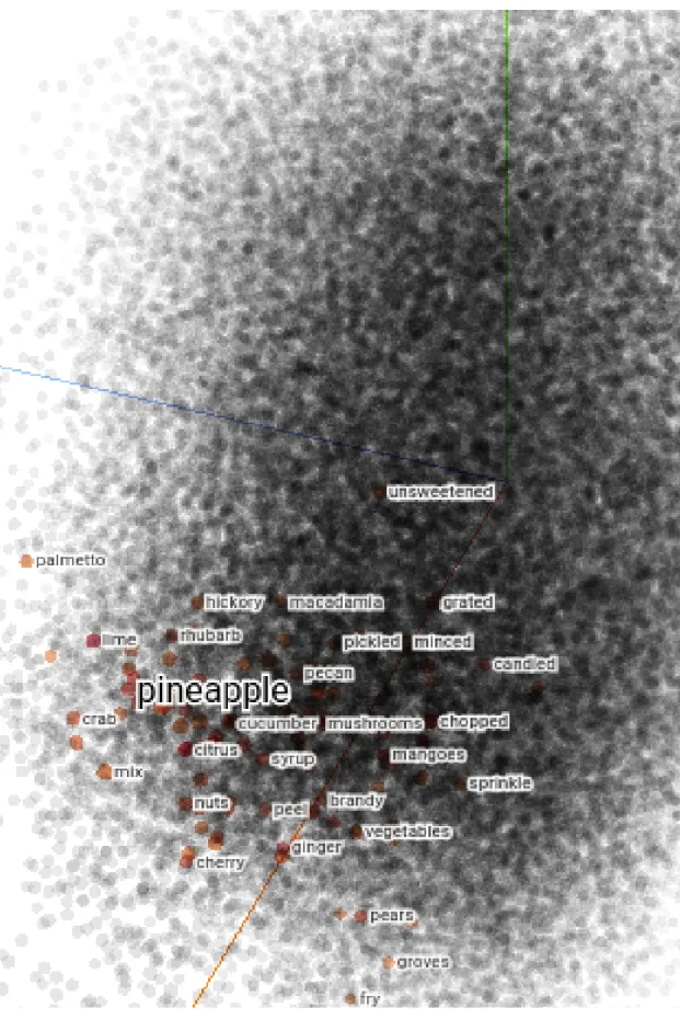
To understand how word embeddings will look like we can visualize a set in 3-dimensions with Tensorboard, a visualizing tool for machine learning provided by (Abadi et al., 2015), using principal component analysis (see Figure 2.3).

It becomes clear that the approach of choosing the vector with smallest cosine similar-ity is only going to make sense if words that mean the same thing or are exchangeable, are mapped closely together.

For sentence- and document-level the same pros and cons as for the word-level ap-ply, with the addition that there is no possibility to create new sentences/documents but only to combine the already existing ones. So using these levels of encoding reduces the granularity and hence also the diversity of the output (when the output is not that long).

Figure 2.3: The image displays the visualization of the word em-beddings with PCA in Tensorboard. Here we have searched for the word pineapple and the words with the closest cosine similarity are highlighted.

Chapter 3

Approach

This chapter describes how we have chosen to approach the problem stated in the beginning of the report. There is also descriptions of the hardware used, how we represent the text, what kind of architectures we have in our different models and finally a motivation of our approach.

3.1

Overall Approach

To answer the questions stated in the goal and problem formulation section, the following methods were used. Firstly we conducted a literature study, were the goal was to see what has been done previously and how it was done. How have they represented the words in the articles? What types of networks did they use? What tools did they use? In what format/type were their output? What were the results? Secondly we investigated and tried to implement generative adversarial networks (GANs), train them for a shorter period of time and finally do further optimization and continue to train the model achieving the best results.

3.2

Setup

The training of the models was done on a machine running Ubuntu 16.04 with a Nvidia Ti-tan X GPU 12 GB. The machine learning library of our choice was Keras with Tensorflow as backend for some models and standalone Tensorflow for some.

3.2.1

Corpus

For the corpus we used roughly one million selected samples from RCV1 (Reuters Corpus Volume 1) (Lewis et al., 2004), 10% of the data selected was used for validation. Some

preprocessing and pruning was done to retrieve articles which mostly consists of sentences (not only tables filled with numbers for instance) and also to convert them from xml to pure text format. We also formatted the texts by encapsulating each article by <START>and <END>tags as well as<TITLE>and</TITLE>tags surrounding the headlines in each article. The result was a mixture of news articles in English published by Reuter between August 20, 1996, and August 19, 1997. The lengths of the articles vary from a few hundred words to a number of thousand words and the topics cover a wide range of the usual English news text.

When the articles are read from disk and being prepared as input to the models, we retrieve the headlines and the corresponding bodies. Firstly we pad or crop the headline to a specified sequence length, then we split the bodies into sequences of the same length (where the last sequence might require padding), with no regards to whether the split oc-curs in the middle of a sentence or not. For padding we use the<PAD>symbol and for unknown tokens we use<UNK>. All characters are also converted to lowercase. To tok-enize the text into sequences we used the following regular expression:

(?![0-9])[\w]+|[0-9;:&.,!?;\%\-\+\=\*\@\£\$)(\/\"\’] Essentially what we do is to split on numbers and other non-alphabetical characters. The reason behind this is to reduce the number of needed word embeddings and we also want the network to figure out for itself a useful combination of words. This in turn also has the effect that the models will have to learn for instance where to put apostrophes.

For the case when we have text as input to the generator instead of noise, we used the same text as for the real samples to the discriminator with the difference that the text to the discriminator is shifted one sequence. This is so that the net will learn an ongoing sequence and so that the output from the generator is compared to the “real” output.

3.2.2

Training

To visualize the training process we used Tensorboard by plotting the loss of both the generator and the discriminator. However, it has been mentioned by Arjovsky et al. (2017) that the loss of the models using the standard GAN does not typical reflect the quality of the generated samples, making the training curves hard to interpret. This was to some extent solved by using WGANs instead but in the end it is the generated text that needs to be inspected. For this reason we have printed samples after every 500 training iterations. The goal for the generator is to generate samples representing an estimate of the distribution of news articles.

For the embeddings we used the pretrained 100-dimensional vectors from Stanford, trained using GloVe (Pennington et al., 2014). In total, 400,000 word embeddings were trained on both Wikipedia and Gigaword 5. We normalized all embedding vectors and some data about the resulting vectors is presented in Table 3.1.

3.3 Models

Standard deviation Mean Min Max

0.09999 0.00119 -0.59135 0.55772

Table 3.1: The table presents some statistics about the values in the word embedding vectors that were used.

3.3

Models

The standard GAN has randomized noise as input to the generator but in our case where we want to generate coherent articles we want to control the input and have the same input being mapped to a single output. We make use of inputs in the form given by Figure 3.1. This is also the same shape of the output from our different models regardless of the input.

3.3.1

Baseline

To make sure that the models we implemented really do make a difference, we created a baseline for both character and word models. This baseline is to simply output random tokens. For the character model, we used a discrete uniform distribution from NumPy (van der Walt et al., 2011) random.randintto give us a index of a character in our vocabulary and for the word embeddings, we used NumPysrandom.uniformto give us values in the range of min-max given by Table 3.1 and mapped these generated embedding vectors to the closest word present in the vocabulary.

3.3.2

GAN model

The model using the standard GAN objective was implemented using Keras (with Tensor-flow as backend). We decided to use the encoder-decoder model where the input to the encoder is mapped to a vector of a given size and then the decoder maps this vector to the final output. We used two LSTM layers with 300 hidden cells in each for both the encoder and decoder. For the discriminator the type of network used was a CNN in accordance to (Zhang et al., 2016) where they stated good performance. For the GAN model, we used text as input in the form of word embeddings.

3.3.3

WGAN models

The other models were implemented using the improved WGAN objective and was incor-porated using Tensorflow. In total four models were trained using this objective. All these models have batch size=512, sequence length=32, optimizer=Adam in common. Two dif-ferent structures of networks were used, one using CNN for both the generator and the critic as well as one using LSTMs for the generator and CNN for the critic. For the LSTM generator we used four layers with a hidden size of 1024 followed by a dense layer and a simple adjustment. By looking at what values the LSTM model produced we noticed that there were not any negative values even though most of the word embeddings contain

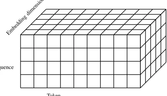
Embedding

dimension

Token sequence

Token

Figure 3.1: The figure illustrates how the input data is fed to the neural nets. The first dimension is the sequence of tokens, the second corresponds to a single token and the third contains the embedding vector for each token. The complete cuboid represents a single batch.

3.3 Models

Model Generator Input Encoding Level

GAN LSTM text word embeddings word

char-noise_in-CNN CNN noise one-hot char

char-text_in-CNN CNN text one-hot char

word-text_in-CNN CNN text word embeddings word word-text_in-LSTM LSTM text word embeddings word

Table 3.2: These are the five models we have trained and evalu-ated. The discriminator has always consisted of a CNN network, since early studies showed it was good for sentence classification, word order and so on. So we have only tried changing the genera-tor from CNN to LSTM. As can also be seen, we have used noise as input only once and this is because we can hopefully reach bet-ter results and have more control of the output if we start with text instead. Otherwise the hyperparameters are the same for every model.

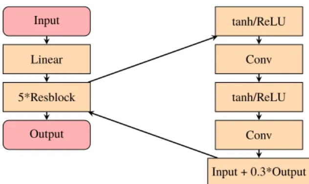
negative values. We therefore added a negative term to the output of the LSTM generator, this term was the minimum value found in the embedding vectors (≈ −0.6). This shifted the possible output of our model so that it now would be able to capture values between −0.6 and 0.6 (in accordance to Table 3.1), corresponding to the span of our embeddings (see Figure 3.3 for an overview). For the CNN generator and discriminator, we use the same structure as in the repository related to Gulrajani et al. (2017) with a few alterations. The activation function in the generator’s residual blocks (resblock) when using word em-beddings will instead of being a ReLU be a tanh, we make this change since that we want to have outputs in the range of [-1, 1] instead of [0, 1] when using character encoding, we will also have asoftmaxoperation before the output (see Figure 3.2). The discriminator makes use of a convolutional layer followed by five resblocks, (ReLU-conv-ReLU-conv) and finishes with a linear layer (see Figure 3.4). For a summary of the models see Table 3.2

The first model used noise as input to the CNN generator and one-hot-character-encoding. The second had text as input to the same type of CNN network and character encoding. The third was the same as the second, with the one-hot-character-encoding replaced by word embeddings of 100 dimensions. The last model made use of the LSTM generator with text as input and word embeddings as encoding.

As we are using the WGAN objective there was no pretraining of neither the generator nor the critic as this objective is more stable than the GAN objective.

Input Linear 5*Resblock Output tanh/ReLU Conv tanh/ReLU Conv Input + 0.3*Output

Figure 3.2: This is the structure of the convolutional generator, we have first a linear/dense mapping to reduce the dimensionality of the input. Then we have five residual blocks consisting of a mixture of tanh/ReLU and convolutional layers (kernel size of 5). The ReLU is used for characters (one-hot) and the tanh is used for words (word embeddings). The output of the residual block consists of the untouched input to the block with the addition of a fraction of the result of the above operations. If we are training a model on characters then there will also be a softmax operation before the output node.

Input 4*LSTM

Dense + Min Emb Value

Output

Figure 3.3: This is the structure of the LSTM generator, it consists simply of four LSTM layers (with 1024 hidden units) followed by a dense layer and finally a bias adjustment of the output.

Input Conv 5*Resblock Linear Output ReLU Conv ReLU Conv Input + 0.3*Output

Figure 3.4: This is how the discriminator looks like. We have a convolutional layer at the top followed by five resblocks (using ReLU) and finally a linear layer.

3.3 Models

3.3.4

Motivation of approach

Our hypothesis is that with these models, using different architectures, we should be able to see which approach is better and more suitable for generating text. The random genera-tor as a baseline will of course not produce any satisfying results, it will rather show what the generator actually needs to do, which is finding a function in the space of word em-beddings that will be an estimate of sequences within news articles. By first investigating how others have used characters and one-hot encodings we want to find current problems and hopefully motivate the use of word embeddings as the next step to take. As far as we know, this is the first time where word embeddings are used as the final output.

As mentioned in the theory, the discreteness of the output has to be solved and the way we do this is by using one-hot encoding for characters and word embeddings for words. We only used 181 characters for the models on character level because we chose to only use the characters present in the Google billion words data set (Chelba et al., 2013).

The GloVe word embeddings encode words that are similar to the same region in the word embedding space and this will hopefully make it easier for the generator as it just has to map the input to the correct part of space, to generate words that are correct given the input. The corpus used as input is encoded by matching words with corresponding word embeddings which are in total 400,000, 100 dimensional vectors. This means that we have a vocabulary of 400,000 words which, unfortunately, will not cover all words such as certain names mentioned in the corpus. This will limit the expressive power of the generator but we think it is a reasonable limitation. Stanford also has pretrained word embeddings of 300 dimensions which should perform better since they contain in a sense more information, however we chose to use only 100 dimensions as to simplify for the generator by reducing the amount of values to learn.

We are then feeding the generator with a sequence of words from the corpus and will let the discriminator affect the generator by the loss it gives for the generated text. The chosen sequence length is going to be a an important parameter as the generator has to draw conclusions on the given input. The reason for choosing both CNN and LSTM networks, was because they both consider the current context in their learning process. The CNN using kernels of a fixed size that strides over the input, while the LSTM is a recurrent neural network and has its own cell state with memory. This is considered when choosing sequence length. If it is given one word then we can not expect it to produce any coherent text. Five words are what the CNN will look at since the kernel has the same size while a LSTM network can learn to remember sequences of different length.

Another parameter that is important is the batch size since we are only updating after one batch, it means that the weights of the neural networks are updated according to the mean loss for the whole batch. If we use a large batch size then the input will vary more since it will contain multiple articles, that do not need to be related. The updates may therefore no longer be satisfactory. A smaller batch size might be more suitable but takes longer time.

Lastly, the reason for only training the models for 15 epochs, was that it was a very time consuming experiment and we were only going to use these models for comparison. Therefore, we decided that there was no need for any further training.

Chapter 4

Evaluation

Here we present how we have chosen to evaluate our models with motivation as well as present the achieved results. We finish this chapter with a discussion of the aforementioned outcome.

4.1

Metrics Used

The best way to test a language model is to use it in a designated environment and measure how much this model improves the overall experience. However this is not always as easily done as said. It can be quite expensive and dependent on the application, hence there exists a need for a metric independent of the environment and simple to obtain, (Jurafsky and Martin, 2016).

4.1.1

Perplexity

As a measure of how good the generated output was compared to the expected “real” output, we used perplexity. We trained N-gram models on both of these documents of text and used these to calculate the probabilities (Equation 4.1) that is then used to calculate the entropy (Equation 4.2) and finally the perplexity (Equation 4.3).

To deal with N-grams the model has not seen, we make use of a smoothing technique called “backoff stupid” (Brants et al., 2007). It essentially works as follows: if the current N-gram is not available then we will revert to using the counts from a simpler (N-1)-gram (multiplied by a backoff factorα. As an examples consider the trigram (“Dogs”, “like”, “treats”) if we don’t have any counts for that trigram we will instead look for counts of the bigram (“like”, “treats”). If also this count is missing we will revert to the base case of the unigram (“treats”), see Equation 4.4.

P(wi|wi−1, ...,wi−N+1)≈ Count(wi,wi−1, ...,wi−N+1) Count(wi−1, ...,wi−N+1) (4.1) H(T)= _|T1_|P logP(k),k =(wi, ...,wi−N+1)∈T (4.2) PP(T)= 2H(T) (4.3)

WhereT is a set of N-grams (sequences of N succeeding words) retrieved from text.

S(wi|wi_i−_−k1₊₁)=          Count(wi i−k+1) Count(wi−1 i−k+1) , ifCount(wi i−k+1)>0 αS(wi|wi−1 i−k+2), otherwise (4.4) To evaluate the models we used a held-out set of sentences retrieved from the corpus used in the training. From this set we extracted 2000 sentences that were used to compare the constructed N-gram models (one for real and one for generated text). We used an α value of 0.4 as proposed by the authors of Brants et al. (2007).

4.1.2

Human evaluation

Because of the complexity of natural languages there exists no good general metric for evaluation of quality and taking into mind that our goal is to produce texts indistinguish-able from man made, we therefore chose to also have a human evaluation where we present text taken from the training corpus and text generated by our models to human volunteers. The task for these volunteers was to judge the text and decide whether they were created by man or machine. Each piece of text was judged upon sentence quality (a subjective mea-surement) and readability/understandability, using grading scales (0-10). Finally a binary decision about the source of the text was asked for (human or machine). All subjects had also been informed that capitalization and other giveaways, that would introduce obvious clues and bias the decision making, had been removed.

4.2

Results

Apart from presenting the results of the metrics introduced in the previous section we will also provide some graphs concerning the distribution of the outputs. First for each model, we present the distribution of both real and generated text, then the generated distribution is presented. To see, in some sense how well structured or correctly the generator was at positioning characters/words, we show the distribution of bigrams for both real and generated text. The distribution of the real text, both characters and words, are from the corresponding expected output so that it really was the text the generator should have produced, or close to. We want to point out that for the distributions of the model using characters with noise as input, there will not be any expected output. Instead we have used the same expected output as when having text as input. This will not affect the results since an optimal generator should produce distributions similar to the expected output. As we are producing text we will also show samples of generated text in Section 4.2.3.

4.2 Results Model Perplexity real Perplexity generated Relative perplexity Unique tokens char-noise_in-CNN* 13.01482 12.97411 0.99687 34 char-text_in-CNN* 13.01482 13.49805 1.03713 32 word-text_in-CNN 578.03741 1108.60480 1.91788 10795 word-text_in-LSTM 578.03741 1356.24841 2.34630 28005 * _{Per character.}

Table 4.1: The table provides the perplexity of the models we have trained. The real perplexity is the calculated perplexity for the real text taken as samples from the corpus and the generated is samples from the generated output. The relative perplexity is defined as Per plexity generated_{Per plexity real} . We used bigrams and 2000 validation sentences.

We are aware of that there is no “fair” way to compare the models using characters and the ones using words. There are fewer characters than words and the perplexity should therefore be lower, as can bee seen in Table 4.1.

4.2.1

Results using characters

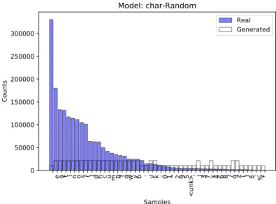
The first model is the random generator, producing characters randomly. This is considered to be the baseline as mentioned in Section 3.3.1. The distribution of randomly generated characters can be seen in Figure 4.1-4.3.

The results of the CNN model using characters and noise as input are presented in Figure 4.4-4.6.

Using text rather than noise as input, keeping the same CNN model with characters, the distributions in Figure 4.7-4.9 were produced.

4.2.2

Results using words

This section contains results of the models when using words represented as word em-beddings as input. The baseline using a random word generator is presented first in Fig-ure 4.10-4.12.

The results of the CNN model using words as input and output are presented in Fig-ure 4.13-4.15.

The distribution of the generated text using the LSTM model with words are presented in Figure 4.16-4.18.

e a t i n o s r l d h c u m p f g w y b . , v k - 0 1 " 2 9 5 <unk> ' j 3 7 x 4 6 8 / q z ( ) $ : % * Samples 0 50000 100000 150000 200000 250000 300000 Counts Model: char-Random Real Generated

Figure 4.1: The image displays the distribution of the 50 most common characters in real text and the number of times these char-acters occurred in generated text from the model using charchar-acters and a random generator.

? l m c w z q r k u g s x e b v p o d h j n y t i f a _ - 4 } 1 > 3 0 & " 7 . ~ ( 2 [ ^ 9 | 8 : ! Samples 0 200000 400000 600000 800000 Counts Model: char-Random Generated

Figure 4.2: The image displays the distribution of the 50 most common characters in generated text from the model using char-acters and a random generator. The reason for the peak on the question mark is that unknown tokens (various random encoded internet characters) were replaced by a question mark.

4.2 Results

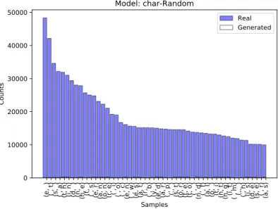
(e, ) ( , t) (s, ) ( , a) (t, h) (i, n) (d, ) (n, ) (h, e) (t, ) ( , s) (e, r) (a, n) (o, n) (r, e) ( , i) ( , o) ( , c) (e, n) ( , w) (e, s) (a, t) (r, ) ( , b) (y, ) (e, d) (a, r) ( , p) (., ) (s, t) (o, r) (t, e) (t, o) ( , ) (n, d) ( , f) (a, l) (o, ) (t, i) (n, t) (n, g) (i, t) ( , m) (,, ) ( , h) (i, s) (d, e) (s, e) ( , r) (a, s)

Samples 0 10000 20000 30000 40000 50000 Counts Model: char-Random Real Generated

Figure 4.3: The image displays the bigram distribution of the 50 most common characters in real text and the number of times these characters occurred in generated text from the model using char-acters and a random generator. Since it is a random generator there is a very low chance of actually follow the bigram distribution of real text, which is why we do not see the generated distribution

e a t i n o s r l d h c u m p f g w y b . , v k - 0 1 " 2 9 5 <unk> ' j 3 7 x 4 6 8 / q z ( ) $ : % * Samples 0 50000 100000 150000 200000 250000 300000 Counts Model: char-noise_in-CNN Real Generated

Figure 4.4: The image displays the distribution of the 50 most common characters in real text and the number of times these char-acters occurred in generated text from the model using charchar-acters, noise as input and a CNN architecture.

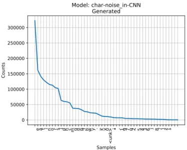
e a t i n o r s l d h c m g u p f b w y . , k v 0 <unk> ¡ " - 1 9 7 q 2 ' 5 4 3 6 j ? 8 / ) z ( ° ? ? Samples 0 50000 100000 150000 200000 250000 300000 Counts Model: char-noise_in-CNN Generated

Figure 4.5: The image displays the distribution of the 50 most common characters in generated text from the model using char-acters, noise as input and a CNN architecture.

(e, ) ( , t) (s, ) ( , a) (t, h) (i, n) (d, ) (n, ) (h, e) (t, ) ( , s) (e, r) (a, n) (o, n) (r, e) ( , i) ( , o) ( , c) (e, n) ( , w) (e, s) (a, t) (r, ) ( , b) (y, ) (e, d) (a, r) ( , p) (., ) (s, t) (o, r) (t, e) (t, o) ( , ) (n, d) ( , f) (a, l) (o, ) (t, i) (n, t) (n, g) (i, t) ( , m) (,, ) ( , h) (i, s) (d, e) (s, e) ( , r) (a, s)

Samples 0 10000 20000 30000 40000 50000 Counts Model: char-noise_in-CNN Real Generated

Figure 4.6: The image displays the distribution of the 50 most common bigrams in real text and the number of times these bi-grams occurred in generated text from the model using characters, noise as input and a CNN architecture.

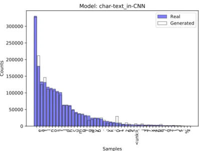
4.2 Results e a t i n o s r l d h c u m p f g w y b . , v k - 0 1 " 2 9 5 <unk> ' j 3 7 x 4 6 8 / q z ( ) $ : % * Samples 0 50000 100000 150000 200000 250000 300000 Counts Model: char-text_in-CNN Real Generated

Figure 4.7: The image displays the distribution of the 50 most common characters in real text and the number of times these char-acters occurred in generated text from the model using charchar-acters, text as input and a CNN architecture.

e t a i n o s r d l h c u p m 0 f . y b w , g k 1 2 v -<unk> j 9 8 " 7 x ' 6 4 3 ( ? $ q ; ? + < : ? Samples 0 50000 100000 150000 200000 250000 300000 Counts Model: char-text_in-CNN Generated

Figure 4.8: The image displays the distribution of the 50 most common characters in generated text from the model using char-acters, text as input and a CNN architecture.

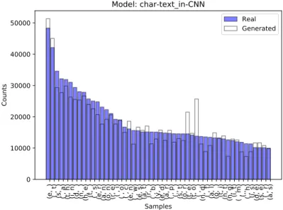
(e, ) ( , t) (s, ) ( , a) (t, h) (i, n) (d, ) (n, ) (h, e) (t, ) ( , s) (e, r) (a, n) (o, n) (r, e) ( , i) ( , o) ( , c) (e, n) ( , w) (e, s) (a, t) (r, ) ( , b) (y, ) (e, d) (a, r) ( , p) (., ) (s, t) (o, r) (t, e) (t, o) ( , ) (n, d) ( , f) (a, l) (o, ) (t, i) (n, t) (n, g) (i, t) ( , m) (,, ) ( , h) (i, s) (d, e) (s, e) ( , r) (a, s) Samples 0 10000 20000 30000 40000 50000 Counts Model: char-text_in-CNN Real Generated

Figure 4.9: The image displays the distribution of the 50 most common bigrams in real text and the number of times these bi-grams occurred in generated text from the model using characters, text as input and a CNN architecture.

the , . to of in a and '' said -- ' on s for at that was it ) ( is <unk> with by

$

from be as he ``

percent

its will but has an _{were would} not

million have tuesday which had are year this we new

Samples 0 10000 20000 30000 40000 50000 60000 70000 Counts Model: word-Random Real Generated

Figure 4.10: The image displays the distribution of the 50 most common words in real text and the number of times these words occurred in generated text from the model using words and a ran-dom generator.

4.2 Results . -- : http @ ) ( & globe.com # nytimes.com - ; ! ? a ap.org d m r ' latimes.com s p $ latwp c hearstdc.com pbpost.com w b l o prodmail.acquiremedia.com amp t rts nytnews e 212 tissottiming.com ad ajc.com chron.com www.startext.net prohibitivo 02107 adv coxnews.com rev Samples 0 2000 4000 6000 Counts Model: word-Random Generated

Figure 4.11: The image displays the distribution of the 50 most common words in generated text from the model using words and a random generator.

(', s) (--, --) (., '') (,, '') (., the) _{(of, the) (in, the) (said, .) (,, the)}

(on, tuesday)

(to, the) (on, the) (for, the) (u., s.) ('', the) (in, a) _{(,, which) (said, the) (he, said) (at, the)} (,, a) _{('', said) (,, and) ('', he) (and, the) (to, be) (by, the) (from, the)} (,, but) _{(said, on) (with, the) (that, the)}

(the, company)

(of, a)

(will, be) (., but) ('', we) (,, said) (., he) (., in) (said, it) (., it) (the, market) (would, be) (the, first) (on, monday)

(,, who) (<unk>, ,) (,, with) (the, government) Samples 0 2000 4000 6000 8000 10000 12000 Counts Model: word-Random Real Generated

Figure 4.12: The image displays the distribution of the 50 most common bigrams in real text and the number of times these bi-grams occurred in generated text from the model using words and a random generator.

the , . to of in a and '' said -- ' on s for at that was it ) ( is <unk> with by

$

from be as he ``

percent

its will but has an _{were would} not

million have tuesday which had are year this we new

Samples 0 20000 40000 60000 80000 100000 120000 Counts Model: word-text_in-CNN Real Generated

Figure 4.13: The image displays the distribution of the 50 most common words in real text and the number of times these words occurred in generated text from the model using words, text as input and a CNN architecture.

the . ,_{this but to and 10 in one that as for} of _{well last}

would not a -- it on said now only

is

even same was

) while ... at company its ' government which they 1 over market so s because year percent

will millionfrom Samples 0 20000 40000 60000 80000 100000 120000 Counts Model: word-text_in-CNN Generated

Figure 4.14: The image displays the distribution of the 50 most common words in generated text from the model using words, text as input and a CNN architecture.

4.2 Results

(', s) (--, --) (., '') (,, '') (., the) _{(of, the) (in, the) (said, .) (,, the)}

(on, tuesday)

(to, the) (on, the) (for, the) (u., s.) ('', the) (in, a) _{(,, which) (said, the) (he, said) (at, the)} (,, a) _{('', said) (,, and) ('', he) (and, the) (to, be) (by, the) (from, the)} (,, but) _{(said, on) (with, the) (that, the)}

(the, company)

(of, a)

(will, be) (., but) ('', we) (,, said) (., he) (., in) (said, it) (., it) (the, market) (would, be) (the, first) (on, monday)

(,, who) (<unk>, ,) (,, with) (the, government) Samples 0 2000 4000 6000 8000 10000 12000 14000 16000 Counts Model: word-text_in-CNN Real Generated

Figure 4.15: The image displays the distribution of the 50 most common bigrams in real text and the number of times these bi-grams occurred in generated text from the model using words, text as input and a CNN architecture.

the , . to of in a and '' said -- ' on s for at that was it ) ( is <unk> with by

$

from be as he ``

percent

its will but has an _{were would} not

million have tuesday which had are year this we new

Samples 0 10000 20000 30000 40000 50000 60000 70000 Counts Model: word-text_in-LSTM Real Generated

Figure 4.16: The image displays the distribution of the 50 most common words in real text and the number of times these words occurred in generated text from the model using words, text as input and a LSTM architecture.

and on the , . 10 _{over than}in s a ( 2 only 1 _{one parts} of said itsto by has --<unk> down

2.5

nearly

'' is '

dlrs least top into entire`` _{largest since} it

monday

will

country were allow them_dropped

6 around for Samples 10000 20000 30000 40000 50000 60000 70000 Counts Model: word-text_in-LSTM Generated

Figure 4.17: The image displays the distribution of the 50 most common words in generated text from the model using words