Banzhaf random forests: Cooperative game theory based random
forests with consistency
Jianyuan Sun
a, Guoqiang Zhong
a,*
, Kaizhu Huang
b, Junyu Dong
aaDepartment of Computer Science and Technology, Ocean University of China, 238 Songling Road, Qingdao 266100, China bDepartment of Electrical and Electronic Engineering, Xian Jiaotong-Liverpool University, SIP, Suzhou 215123, China
h i g h l i g h t s
• A novel random classification forests algorithm, called Banzhaf random forests (BRFs), is proposed.
• The Banzhaf power index is employed to evaluate the power of each feature by traversing possible feature coalitions.
• The consistency of BRFs is proved.
a r t i c l e i n f o
Article history:
Received 29 August 2017
Received in revised form 14 April 2018 Accepted 8 June 2018
Available online 28 June 2018
Keywords: Random forests Cooperative game Banzhaf power index Consistency
a b s t r a c t
Random forests algorithms have been widely used in many classification and regression applications. However, the theory of random forests lags far behind their applications. In this paper, we propose a novel random forests classification algorithm based on cooperative game theory. The Banzhaf power index is employed to evaluate the power of each feature by traversing possible feature coalitions. Hence, we call the proposed algorithm Banzhaf random forests (BRFs). Unlike the previously used information gain ratio, which only measures the power of each feature for classification and pays less attention to the intrinsic structure of the feature variables, the Banzhaf power index can measure the importance of each feature by computing the dependency among the group of features. More importantly, we have proved the consistency of BRFs, which narrows the gap between the theory and applications of random forests. Extensive experiments on several UCI benchmark data sets and three real world applications show that BRFs perform significantly better than existing consistent random forests on classification accuracy, and better than or at least comparable with Breiman’s random forests, support vector machines (SVMs) and k-nearest neighbors (KNNs) classifiers.
©2018 Elsevier Ltd. All rights reserved.
1. Introduction
Machine learning is an important sub-area of artificial intelli-gence. It includes many branches, such as ensemble leaning and deep learning. In recent years, a great deal of work shows the ef-fectiveness of deep learning in solving practical problems ( Amoze-gar & Khorasani, 2016;Bulo & Kontschieder, 2014;Kim, Jang, & Lee, 2016; Mcquoid, 1993; Pavel, Schulz, & Behnke, 2017; Roy & Todorovic, 2016; Scardapane & Di, 2017). However, in order to obtain better performance, it tends to combine the ideas of deep learning and ensemble learning. For instance, some work tries to improve the performance of deep learning models based on ensemble learning (Amozegar & Khorasani, 2016; Mcquoid, 1993; Scardapane & Di, 2017), while some uses deep learning models for feature extraction and ensemble learning models for
*
Corresponding author.E-mail address:[email protected](G. Zhong).
classification or regression (Bulo & Kontschieder, 2014;Roy & Todorovic, 2016). In this paper, we focus on an ensemble learning method, random forest, which is mainly based on the combination of several independent decision trees (Breiman, 2001).
As a general classification and regression tool, the random forests algorithm and its variants (Ayerdi & Grana, 2014;Ristin, Guillaumin, Gall, & Van Gool, 2016; Zhang & Suganthan, 2014) have been successfully applied in many fields, such as computer vision (Dollar & Zitnick, 2014;Hallman & Fowlkes, 2015;Shotton, Sharp, Kipman, Fitzgibbon, Finocchio, Blake, Cook, & Moore, 2013; Zikic, Glocker, & Criminisi, 2013) and pattern recognition (Bosch, Zisserman, & Muoz, 2007;Shotton, Johnson, & Cipolla, 2008;Yin, Criminisi, Winn, & Essa, 2007). Nevertheless, the theory of random forests lags far behind their applications. Fortunately, Biau et al. have made a breakthrough in theoretical research of the random forests algorithms in recent years (Biau, 2012;Biau, Devroye, & Lugosi, 2008). However, as they mainly focus on the consistency of
https://doi.org/10.1016/j.neunet.2018.06.006
the random forests algorithms, the proposed algorithms generally perform not very well.
In this paper, we propose a new random classification forests al-gorithm based on the cooperative game theory, and call it Banzhaf random forests (BRFs). BRFs are formed with a number of Banzhaf decision trees (BDTs). For each BDTs, we adopt the Banzhaf power index to evaluate the ‘‘best’’ feature at each tree node. The Banzhaf power index is a method to calculate solution of the cooperative game, which can be used to explore the internal structure of the feature variables. More importantly, based on previous work on the consistency of classifiers (Biau, 2012;Biau et al., 2008), we have proved the consistency of BRFs.
The remainder of this paper is organized as follows. In Section2, we review some related work on random forests algorithms. In Section3, we describe two critical issues for constructing decision trees in random forests. In Section4, we introduce the proposed BRFs algorithm in detail. Section5is devoted to the proof of the consistency of BRFs. In Section 6, we report the experimental results obtained by BRFs and the compared algorithms on several UCI data sets. Section7concludes this paper.
2. Related work
The original random forests algorithm (Breiman, 2001),
which combines several classification and regression trees (CART) (Breiman, Friedman, Stone, & Olshen, 1984) or C4.5 deci-sion trees (Salzberg, 1994) using bagging (Breiman, 1996), is pro-posed by Breiman. The construction of random forests algorithm is mainly based on three pieces of existing work: the feature selection work ofAmit and Geman(1997), the random subspace method of Ho(1998) and the method of random split selection ofDietterich (2000). Later on, Criminisi et al. present a unified framework for random forests models (Criminisi, Shotton, & Konukoglu, 2012).
Random forests models have an excellent classification and re-gression performance. Therefore, they have been applied to a wide variety of real world applications (Criminisi & Shotton, 2013; Cut-ler, Edwards Jr, Beard, CutCut-ler, Hess, Gibson, & LawCut-ler, 2007;Prasad, Iverson, & Liaw, 2006;Svetnik, Liaw, Tong, Culberson, Sheridan, & Feuston, 2003). Although random forest algorithms have achieved great successes in practice, the mathematical properties behind them are difficult to be analyzed (Breiman, 2004). There are two main properties of the theory related to random forests models. The first is the consistency of the models, i.e. whether they can converge to an optimal solution as the data set grows infinitely large. The second is the rate of the convergence. In this work, we focus on the consistency aspect of the proposed BRFs algorithm. Note that, Biau et al. have showed that the consistency of Breiman’s random forests cannot be theoretically guaranteed (Biau et al., 2008).
In recent years, many researchers have devoted efforts to the study of the consistency of random forests algorithms. Mein-shausen has presented a consistent random regression forests algorithm, called quantile regression forests (Meinshausen, 2006). Ishwaran and Kogalur have demonstrated that their proposed algorithm, survival forests, possesses consistency (Ishwaran & Kogalur, 2010). In addition, Denil et al. have developed an online version of the random forests algorithms and proved its consis-tency (Denil, Matheson, & de Freitas, 2013b). Moreover, a new ran-dom regression forests algorithm was given byDenil, Matheson, and De Freitas(2013a). However, the consistency of these existing random forests algorithms only focuses on the online learning and regression problems. A significant contribution to the theory of random forests is the work by Biau et al.(2008), which proves the consistency of various randomized ensemble classifiers and investigates the consistency of bagging rules (Breiman, 1996). Biau et al. have also proposed two consistent random forests classifiers:
the pure random forests and the scale-invariant version of the random forests (Biau et al., 2008). More importantly, Biau et al. suggest that various greedy random forest classifiers, including Breiman’s random forests classifier, are inconsistent. To remedy the inconsistency of these random forests classifier, some tech-niques need to be employed (Györfi, Devroye, & Lugosi, 1996). For instance, the decision trees in random forests use different stopping rules instead of growing every decision tree down to nodes with a single data point.
In this paper, we propose an innovative random classification forests algorithm based on the cooperative game theory. It uses the Banzhaf power index to evaluate the power of each feature by traversing all possible feature coalitions, and the midpoint of the most powerful feature is used to split the node. According to the existing theoretical work, the consistency of the proposed random forests algorithm has been proved. Furthermore, extensive experiments show that the performance of the proposed random forests algorithm is significantly better than that of existing con-sistent random forests, and better than or at least comparable with Breiman’s random forests and other state-of-the-art classifiers.
3. Two critical issues in random forests
In general, when some decision trees are employed in a random forests algorithm, two critical issues need to be considered. The first one is the method for splitting the tree nodes, and the second one is the method for injecting randomness into the trees. At the same time, the strategic choice of these two critical issues also determines whether a random forests algorithm is consistent.
Specifying a method for splitting tree nodes needs to select the shapes of candidate splits and a criterion for evaluating the quality of each candidate split point or feature. Typical choices are to use axis aligned splits, where sample data are routed to sub-trees depending on whether or not they exceed a threshold value of a chosen feature; or linear splits, where a linear combination of fea-tures is compared with a threshold to make a decision (Breiman, 2001). The threshold value in either case can be chosen randomly or by optimizing a function of the data in the tree nodes.
For the used split point, a simple method is to choose among the candidate split points at random, such as a random forests algorithm of Biau et al. (2008). A more common method is to choose the ‘‘best’’ split points, which optimizes a purity function to travel the possible candidate split point of each feature in a tree node. A typical choice is to maximize the Gini index or the information gain ratio (Breiman, 2001;Friedman, 2001;Geurts, Ernst, & Wehenkel, 2006). Recently, Biau(2012) proposed a new method to split the tree node in their random forests model (called Biau12, in our paper). They had not used the traversal way to compute the ‘‘best’’ split point. Alternatively, the midpoint of the most important feature was used to split the node. In this way, Biau12 algorithm can achieve consistency. In our paper, based on the theoretical results of Biau et al., we proved the consistency of the proposed BRFs algorithm. In particular, to ensure that the proposed BRFs algorithm has consistency, the midpoint value of the ‘‘best’’ feature was used as split point to expand tree nodes.
In addition, Breiman claims that randomness can help to re-duce the correlation between tree classifiers in a random forests algorithm, and meanwhile, maintain reasonable strength of each tree (Breiman, 2001). Therefore, injecting randomness is very important to improve the performance of random forests models. In general, injecting randomness into each tree can be achieved in several ways. Which feature to be chosen for splitting the tree node can be random, and the split point can be chosen either randomly or by optimization over some or all of the data at each tree node. In this work, we randomly select some data samples and features to construct the decision trees.
4. Banzhaf random forests
In this section, we present the construction rules of Banzhaf ran-dom forests (BRFs). Banzhaf ranran-dom forests are formed by combin-ing the prediction of several Banzhaf decision trees (BDTs). The idea of constructing the BDTs mainly motivated by Banzhaf power index that comes from the cooperative game theory. Therefore, first, we start with some basic concepts of the cooperative game theory and the Banzhaf power index. Second, we introduce the method of constructing the randomized BDTs. Third, the construction rules of BRFs are given. Finally, we discuss the computation issue and present the prediction method of BRFs.
4.1. Some basic concepts of the cooperative game theory
Cooperative game is a game where groups of players (‘‘coali-tions’’) may enforce cooperative behavior, while the game is a competition between coalitions of players rather than between individual players. Cooperative game theory mainly searches for an ‘acceptable’ way to distribute gains to each individual player in the cooperative game (Chalkiadakis, Elkind, & Wooldridge, 2011). The mathematical definition of cooperative games (Chalkiadakis et al., 2011) can be read as follows.
Formally, the cooperative game Γ
=
(N, γ
) consists of a finite set of playerN= {
1,
2, . . . ,
n}
, called the grand coalition,and a characteristic function
γ
:
2N→
R. For each subsetS
⊆
N,γ
(S) represents the profit achieved by the players of S⊆
N by accomplishing the task together. In general, the goal in a cooperative game is to distribute the total gainsγ
(N) to each playeri(i=
1,
2, . . . ,
n) who belongs to the grand coalitionNin a fair and reasonable way.Obviously, the grand player setN gets profit more than that of any player subsetS
⊂
N in a cooperative gameΓ=
(N, γ
), i.e.,γ
(N)> γ
(S). Only meeting this condition, the players inN are willing to cooperate. Otherwise, no cooperation is necessary. In particular, a game is a cooperative game, which need to satisfy the superadditivity (Saad, Han, Debbah, & Hjorungnes, 2009). Superadditivity implies that, given any two disjoint player subsets S1andS2, if coalitionS1⋃
S1forms, then it can guarantee at least
the profit that is obtained by the disjoint coalitions separately. i.e.,
γ
(S1)⋃
γ
(S2)≥
γ
(S1)+
γ
(S2),∀
S1⊂
N,
S2⊂
N andS1
∩
S2=
∅. Therefore, how much profit to be obtained and howto distribute the gains are an important factor to the players in the cooperation.
Moreover, for the distribution of total gains, different require-ments of fairness and rationality yield different solution concepts for the cooperative game, such as ‘the nucleolus’, ‘the Shapley value’, ‘Banzhaf power index’ and other concepts. Among these solution concepts, the nucleolus and the Shapley value focus on providing the expected payment for each player in the coalition, while the Banzhaf power index focuses on evaluating the power or importance of each player in the coalition (Feltkamp, 1995). In particular, the Banzhaf power index focuses more on the fairness of the distribution gains. For the proposed BRFs algorithm, we try to search the node feature with the strongest discriminative ability for classification tasks, according to the intricate and intrinsic interrelation among candidate features. That is, the most powerful or important feature is selected as the split feature at each tree node. Therefore, in this work, we use the Banzhaf power index to evaluate the power or importance of the candidate features at each tree node.
The definition of Banzhaf power index is described inBanzhaf III (1964). The original Banzhaf power index is used to evaluate the power of players in a simple game. The simple game is a coop-erative game due to satisfying the superadditivity (Saad et al., 2009). A simple game Γ
=
(N, γ
) consisting of a player setN
= {
1,
2, . . . ,
n}
with|
N| =
n, the coalitionSwith value 1 isconsidered to be ‘winning’, and that with value 0 is considered to be ‘losing’, i.e.
∀
S⊆
N,γ
(S)=
1 andγ
(S)=
0, respectively. The phenomenon that coalitionS∪{
i}
wins butSloses is called a swing of playeri∈
N, because the playeriin the coalitionS∪{
i}
is crucial to its ‘winning’. In fact, the Banzhaf power index of a playeri∈
N is the probability of swings of playeri. Here, the symbolβ
i(Γ) is used to represent the Banzhaf power index of playeri∈
N, and it is given byβ
i(Γ)=
1 2n−1∑
S⊆N\{i} ∆i(S),
(1)where 2n−1 represents the total number of player subsetsS
⊆
N
\{
i}
and∆i(S) is the marginal contribution of playeri, i.e.∆i(S)=
γ
(S∪ {
i}
)−
γ
(S).From Eq.(1), the Banzhaf power index of playeri(i
∈
N) is used to count the number of ‘winning’ coalitions when the playerijoins in the ‘losing’ coalitionsS⊆
N\ {
i}
. To find the most powerful playerithat can make the majority of coalitions ‘winning’, the normalized Banzhaf power indexζ
i(Γ) is defined asζ
i(Γ)=
β
i(Γ)∑
i∈Nβ
i(Γ),
(2) where∑
i∈N
β
i(Γ) is the total number of ‘winning’ coalitions of all players in the game.Banzhaf power index has a particularly attractive inter-pretation—it measures the power of each player in a cooperative game, i.e. the probability that this player yields a good or bad result to a game. Some famous and vivid examples inBanzhaf III(1964) may help the readers for a better understanding of the Banzhaf power index. In this paper, in order to construct each BDT, we employ the Banzhaf power index to evaluate the power of the candidate features at each tree node.
4.2. Construction of BDTs
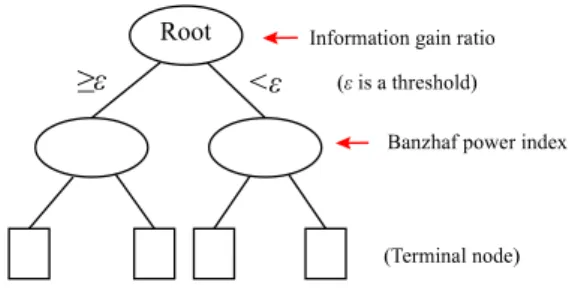
BRFs are composed of several Banzhaf decision trees (BDTs). Fig. 1shows the structure of a single BDTs. For the root node, the ‘‘best’’ feature is selected by the criterion of the information gain ratio. For all of the other nodes except the leaves, the ‘‘best’’ features (players in the cooperative game) are selected by the Banzhaf power index. At each step, the midpoint value of the ‘‘best’’ feature is selected as the split point, which can be considered as a threshold
ε
. If there is only one data point in each tree node or a predefined number of cuts has been reached, then the tree stops growing.We apply Eq.(1)to the process of constructing BDTs. At each tree node, the Banzhaf power index of featurefi is computed as follows.
Each step of constructing the BDTs can be modeled as a simple gameΓ
=
(N, γ
), which consists of a feature player setN=
{
f1,
f2, . . . ,
fn}
. i.e.,γ
(S)∈ {
0,
1}
,∀
S⊆
N andγ
(N)=
1. In particular, the simple game satisfies the superadditivity (Saad et al., 2009). Therefore, the problem of computing the Banzhaf power index of features at each node of BDTs is a cooperative game. Then, let the coalitionSbe a subset of the features andfi(fi̸∈
S) be a feature to be estimated.Whether featurefileads a coalitionSto enter the ‘winning’ state can be measured by the ratio
σ
=
µ
fi(S)/ρ
fi(S), whereµ
fi(S) is the number of features (belonging to the coalitionS) interdependent with the featuresfi(fi̸∈
S), andρ
fi(S) is the total number of features in the coalitionS. For convenience, the symbolτ
is used to represent the splitting threshold for the ratioσ
, and we setτ
=
1/
2. Ifσ < τ
, the coalitionS∪ {
fi}
is ‘losing’, otherwise, it is ‘winning’, i.e. ∆fi(S∪
fi)=
{
1σ
≥
τ
;
0σ < τ.
The threshold
τ
=
1/
2 means, if more than half of the features of a coalitionSare interdependent withfi, thenfijoining can make coalitionSenter the ‘winning’ state. Hence, for simplicity of the computation, we specify∆i(S) for a single coalitionS⊆
N\ {
fi}
in Eq.(1)as∆i(S)
=
γ
(S∪ {
i}
)−
γ
(S)=
{
1
σ
≥
τ
;
0
σ < τ.
(3)In this work, we use the conditional mutual information to evaluate the interdependence between a single featurefi
∈
N\
S and the feature playerfj∈
S⊆
N. In general, the conditional mutual informationI(X;
Y|
Z) is defined as information shared byrandom variables X and Y when variable Z is given. It can be
formally defined as I(X
;
Y|
Z)=
∑
x∈X∑
y∈Y∑
z∈Z p(x,
y,
z) log p(x,
y|
z) p(x|
z)p(y|
z).
Conditional mutual information is also widely used to measure the reduction of the uncertainty ofXdue to the knowledge ofY
whenZis given.
In our paper, the conditional mutual information is used to measure the interdependency between a single feature playerfi
̸∈
Sand the target class labely, given feature playerfj∈
S. It is defined byI(fi
;
y|
fj)=
p(fi,
fj,
y) logp(fi
,
y|
fj)p(fi
|
fj)p(y|
fj).
(4)Two feature variablesfi andfjare interdependent on each other, if the relevance betweenfiand the target classyincreases given
fj, i.e.I(fi
;
y)≤
I(fi;
y|
fj), whereI(fi;
y) is the mutual information between the featurefiand the class labely.By Eqs.(1),(3),(2)and(4), we can obtain the Banzhaf power in-dex of each candidate feature for each tree node. More concretely, this computation process is described in Algorithm 1.
Algorithm 1: Selecting the best feature using the Banzhaf power index
Input: A tree node contains data setDnwith feature spaceF and the data labelsy.
Output:
β
: Banzhaf power index vector ofF.β
=
0,τ
=
12;
Foreach featurei
∈
FdoCreate coalitions set
{
S1, . . . ,
St}
overF\ {
i}
;Foreach featureSj
∈ {
S1, . . . ,
St}
doCalculate marginal function∆i(Sj) using Eq. (3) and Eq. (4);
End
Calculate the Banzhaf power index
β
iusing Eq. (1);End
Normalized the value
β
iusing Eq. (2) to obtainζ
i; Choose the best feature with maxiζ
ifor this tree node.For clarity, we give an example to demonstrate how the Banzhaf power index can be used to evaluate the power of a feature. Given a cooperative feature gameΓ
=
(N, γ
) with the feature player setN= {
f1,
f2,
f3,
f4}
. Our goal is to calculate the Banzhaf powerindex of the featuref4. For all coalitionsS
⊆
N\ {
f4}
, the totalnumber of possible coalitions of feature subsetsN
\ {
f4}
is 8.Assume that the featuref4can make the coalitions
{
f2}
,{
f2,
f3}
and{
f1,
f2}
enter the ‘winning’ state, i.e. each coalition has half of itsFig. 1.A Banzhaf decision tree.
features interdependent with featuref4. Then the Banzhaf power
index off4can be computed as
β
f4(Γ)=
1 24−1∑
S⊆N\{f4} ∆f4(S)=
3/
8.
where∑
S⊆N\{f4}∆f4(S)=
∑
S⊆N\{f4}(γ
(S∪ {
f4}
)−
γ
(S))=
1
+
1+
1=
3. Similarly, the Banzhaf power index of other features can be computed in a similar way.4.3. Banzhaf random forests algorithm
Given a training data setDn
=
(Xi,
Yi)ni=1, includingnsam-ples with dimensionalityM, the learning of BRFs is based on the general technique of bootstrap aggregating, or bagging, and the constructed BDTs. The BRFs algorithm can be formally described as follows.
•
Using the bagging method to generatentreesubsets,{
d1,
d2,
. . . ,
dntree}
, wherentreeis the number of trees in BRFs.Con-cretely, for each tree, randomly samplingDnforntimes with replacement.
•
For each data setdi, a Banzhaf decision tree is built. Before the decision tree construction, randomly sample a subspace ofh=
round(log2(M)+
C) (h≪
M) features from the avail-able features presented indi, whereC∈
Ris a parameter. For the root node, the ‘‘best’’ feature is selected by the criterion of information gain ratio. For the other nodes except the terminal ones, the ‘‘best’’ feature is selected among thehfeatures based on the Banzhaf power index. The midpoint value of the ‘‘best’’ feature is used as a split threshold to generate left and right child nodes. Repeat this process until reaching the user-set limit (i.e. the percentage of incorrect points or a minimal number of samples at a node).
•
Integrating ntree BDTs h1(d1),
h2(d2), . . . ,
hntree(dntree) to form a Banzhaf random forest (BRF), and this BRF uses the majority votes ofntreeBDTs to obtain the class prediction for a new sample.It is easy to see that the BRFs algorithm is similar to the original random forests algorithm by Breiman(2001). Both of them use bootstrap aggregating, i.e. the bagging ensemble method. The main difference between them is the way of selecting the split point (threshold) for each tree node. For the original random forests, the information gain ratio is employed to traverse each possible split point at each candidate feature, accordingly, the ‘‘best’’ split point and the corresponding feature is obtained. While BRFs algorithm employs a different way to obtain the split point at each tree node. BRFs first use the Banzhaf power index to evaluate the ‘‘best’’ fea-ture, and then the midpoint value of the ‘‘best’’ feature is selected as the split point.
4.4. Computational issue
To evaluate the power of each feature, it is necessary to calculate the proportion of the ‘winning’ coalitions. Theoretically, calculat-ing the Banzhaf power index requires summcalculat-ing over all possible feature subsets, which may lead to high computational complexity. However, empirically, it is unnecessary to consider empty-set and large coalitions. In most cases, there is a small probability that a single featurefiresults in a large coalition to be ‘winning’. Hence, we set a bound
ϖ
for the coalition size. To this end, Eq.(1)can be redefined asβ
i(Γ)=
1|
Πϖ|
∑
S⊆Πϖ ∆i(S),
whereΠϖis the subset of the feature setF
\ {
fi}
(except∅), witha number of elements less than or equal to
ϖ
.Moreover, in our proposed method, whether a coalition win or not depends on the number of features increasing (or reducing) its associate with the target class when the condition is given. Therefore, at each node of BDTs, the number of winning coalitions containing only one member (denoted asM1) that can be
calcu-lated with time complexityO(n), wherendenotes the number of features at the corresponding tree node. Then, we can calculate the number of winning coalitions that including more than one member based onM1according to the knowledge of combinatorial
mathematics and dynamic programming technique. In particular, dynamic programming is an efficient programming technique for solving the combinatorial problems (Cormen, Leiserson, Rivest, & Stein, 2009). For example,M2can be calculated asM2
=
CM21+
CM11
×
C 1n−M1, whereCrepresents the number of combinations. In
this way, each BDTs in BRFs can be constructed with low compu-tational complexity.
More specifically, to determine the value of
ϖ
for most appli-cation, we used 5-fold cross-validation to choose the value ofϖ
for all of the experiments (shown in Section6). The experimental results demonstrated that, whenϖ
∈ [
3,
5]
, the performance of BRFs is satisfactory. Thus, we suggest a range of[
3,
5]
forϖ
in most of the applications. Based on the above discussion, the computational complexity of constructing BRFs is acceptable for real world applications.4.5. Prediction
We denote a Banzhaf decision tree (BDT) created in the BRFs algorithm asgn. To make a prediction for a query pointx, each BDT computes, for each classk,
η
k n(x)=
1 N(An(x))∑
(Xi,Yi)∈An(x)δ
(Yi=
k),
where (Xi
,
Yi) is i.i.d. pairs of random variables,X (the feature vector) takes its value in R(M+1), Y (the label) is a multi-classrandom variable,An(x) denotes the leaf node of the tree containing
x, andN(An(x)) is the number of points that are located inAn(x). The tree prediction is then the class that maximizes the value
η
kn, i.e.gn(x)
=
arg max k{
η
kn(x)}
.
BRFs predict the class that receives the most votes from the indi-vidual BDT.
5. Consistency of BRFs
In this section, we discuss and present the theoretical results about the consistency of Banzhaf random forests (BRFs). In partic-ular, under some assumptions, we prove that BRFs are consistent.
5.1. Theoretical results
We denote the Banzhaf decision tree (BDT) created by the BRFs algorithm fromndata points asgn. Asnvaries, a sequence of BDT classifiers can be obtained, i.e.
{
gn}
. Then, we focus on showing that the sequence{
gn}
is consistent. According to the work of Devroye et al. (Györfi et al., 1996), a sequence{
gn}
of BDT classifiers is consistent, when the probability of error ofgn converges to the Bayes riskL∗, i.e.
L(gn)
=
P(gn(X, θ,
Dn)̸=
Y)→
L∗
,
asn
→ ∞
, where (X,
Y) is a random test data point,θ
represents the randomness of constructing BDT, such as randomly selecting a group of features to evaluate the ‘‘best’’ features for each node, andDnis the training data set. The Bayes riskL∗is the minimum of the prediction error of the Bayes classifier for the distribution of (X,
Y), which makes predictions by choosing the class with the highest posterior probability,g(x)=
arg maxkP(Y=
k|
X=
x).For more explanation about this setting, please refer to the work byGyörfi et al.(1996).
In order to reduce the complexity of the problem, we try to reduce the problem of proving the consistency of multi-class clas-sifier
{
gn}
to prove the consistency of the transformed two class classification problems. Inspired by the work ofDenil et al.(2013b), we give the lemma as follows.Lemma 1. Suppose the probability estimates,
η
kn(x), for each class posteriorη
k(x)=
P(Y=
k|
X=
x), is consistent (as n→ ∞
, tends to the class Bayes probability). Then the classifiergn(x)
=
arg max k{
η
kn(x)}
is consistent for the corresponding multi-class classification problem as n
→ ∞
.Proof. In the case, where each class posterior
η
k(x) is equal, there is nothing to prove, since all results have the same probability of error. So, suppose there is at least onek such thatη
k(x)<
η
g(x)(x)(g(x)=
arg max k{
η
k(x)}
) and define m(x)=
η
g(x)(x)−
max k{
η
k(x)|
η
k(x)< η
g(x)(x)}
,
mn(x)=
η
ng(x)(x)−
maxk{
η
k n(x)|
η
k(x)< η
g(x)(x)}
,
wherem(x) is the margin function for each class which measures how much better the best result is than the second best result. By assumption, the probability estimates of each class posterior is consistent, som(x)
≥
0. Similarly, the functionmn(x) measures the margin for multi-classgn(x). Ifmn(x)>
0, thengn(x) has the same probability of error as the Bayes classifier. Accordingly, we just need to provemn(x)>
0.Based on the above guarantees, there is some
ϵ
such thatm(x)>
ϵ
. Because the probability estimatesη
kn(x) of each class posterior
η
k is consistent, by makingnlarge it can satisfyP(
|
η
nk(X)−
η
k(X)|
< ε/
2)≥
1−
δ,
whereδ
∈
(0,
1) is arbitrary, then we havemn(X)
=
η
ng(X)−
max k{
η
kn(X)|
η
k(X)< η
g(X)(X)}
≥
(η
g(X)−
ϵ/
2)−
max k{
η
nk(X)+
ϵ/
2|
η
k(X)< η
g(x)(X)}
=
η
g(X)−
max k{
η
k(X)|
η
k(X)⟨
η
g(x)(X)} −
ϵ
⟩
0.
Since
δ
∈
(0,
1) is arbitrary, this means that the risk of gn(x) converges in probability to the Bayes risk. □Lemma 1allows us to transform the proof of the consistency of multi-class tree classifier to prove the consistency of the corre-sponding two class classifiers, i.e. given a set of classes
{
1, . . . ,
c}
, we can re-assign the labels by using the map (X,
Y)↦→
(X,
I(Y=
k)) for any k
∈ {
1, . . . ,
c}
. We solve a two class classification problem,η
k(x)=
P(Y
=
1|
X=
x) is equal to learnη
kn(x) in the original multi-class classification problem. Then we only need to show that the sequence{
gn}
of BDT classifiers is consistent for the corresponding two-class problem. In addition, according to the work ofBiau et al.(2008), for the two class random forests classifier, if the number ofntreeis large, the random forests classi-fier takes a majority vote to obtain the classification result, which can be well approximated by the averaged classifier. As shown in Biau et al.(2008) that consistency of a random forests classifier is preserved by averaging, we haveLemma 2.Lemma 2. Assume that the sequence
{
gn}
of tree classifiers iscon-sistent for a certain distribution of (X
,
Y). Then the voting random forests classifier gn(ntree) (for any value of ntree) and the averagedforests classifier gnare also consistent.
Proof. See that for Proposition 1 inBiau et al.(2008). □
According toLemma 2, we can state the main theoretical result about BRFs. In addition, to prove the consistency of BRFs, it is sufficient to prove the consistency of the base tree classifier (BDT)
gnbased onLemma 2. Before giving our main theorem, we recall the construction method of the Banzhaf decision trees (BDTs) and give some mild assumptions as follows.
All nodes of the individual BDT can be seen as associated with rectangular cells, such that at each step of the construction of the individual BDT, the collection of cells associated with the external nodes of the BDT forms a partition ofdn
∈ [
0,
1]
h⊆
Dn. Then, the root node of BDT is[
0,
1]
hitself. In addition, the Banzhaf power index is used to evaluate the power of candidate features for each tree node. In fact, the Banzhaf power index of each candidate feature can be seen as a probability that each candidate feature may be chosen at each node, i.e. at each node, each candidate featureXj is chosen according to the value of a Banzhaf power indexζ
nj∈
(0,
1) (refer to Eq.(2)), in particular,∑
hj=1
ζ
nj=
1. Furthermore, because BDT chooses the midpoint of feature as the split point to expand tree at each node, then we assume that each BDT has 2⌈log2kn⌉(≈
kn) terminal (leaf) nodes, and letKnj(X
, θ
) denote the number of times the leaf nodeAn(X, θ
) is split on thej
−
thfeature (j=
1, . . . ,
h). Then, conditioned onX,Knj(X, θ
) has a binomial distributionB(⌈
log2kn⌉
, ζ
nj). Inspired by the work of Biau et al. (Biau, 2012) and based on the above assumptions, our main theorem is given as follows.Theorem 1. Assume that the distribution of X has support on
[
0,
1]
h⊆
Dn. Then the BRFs estimate gn is consistent whenever log2kn→ ∞
and kn/
n→
0as n→ ∞
.Proof. ByLemma 1, the consistency of multi-class classifier can be transformed to the consistency of the corresponding two-class classifiers. In addition, for the two-class situation,Lemma 2allows us to transform proving the consistency of BRFs into proving the consistency of base tree classifiergn. Therefore, we only need to prove that the individual BDT classifier is consistent.
To prove the consistency of BDT, we recall a general consistency theorem for partitioning tree classifiers proved in Györfi et al. (1996, Theorem 6.1). According to this theorem, the BDT classifier
gn is consistent if both diam(An(X
, θ
))→
0 in probability andNn(X
, θ
)→ ∞
in probability, whereAn(X, θ
) is the rectangularcell (node) of the tree partition containingXand
Nn(X
, θ
)=
n∑
i=1
I{Xi∈An(X,θ)}
is the number of data point falling in the same cell asX.
First, we prove thatNn(X
, θ
)→ ∞
in probability, whereθ
denotes the partition of BDT. Assume that the number of partition is⌈
log2kn⌉
, then a single BDT has exactly 2⌈log2kn⌉ cells (nodes),
i.e. A1
, . . . ,
A2⌈log2kn⌉. LetN1, . . . ,
N2⌈log2kn⌉ denote the number ofdata points among X
,
X1, . . . ,
Xn falling in these 2⌈log2kn⌉ cells. Since the data pointsX,
X1, . . . ,
Xnare independent and identically distributed, fixingθ
, the conditional probability of data pointXfalls in theith cell is equal toNi/
(n+
1). Thus, for every fixedt≥
0,P(Nn(X
, θ
)≤
t)=
E[
P(Nn(X, θ
)≤
t|
θ
]
=
E[
∑
i=1,...,2⌈log2kn⌉:Ni<t Ni n+
1]
≤
t2 ⌈log2kn⌉ n+
1≤
2tkn n+
1,
which converges to 0 by assumption onkn
/
n→
0.Next, we show thatdiam(An(X
, θ
))→
0 in probability. To this aim, it is sufficient to show that the size of the each dimension feature of the rectangular cell containing Xconverges to 0. LetVnj(X
, θ
) denote the size of thej−
th(j=
1, . . . ,
h) dimension fea-ture. Then, we only need to show thatVnj(X, θ
)→
0 in probability for allj=
1, . . . ,
h. In addition, we haveVnj(X
, θ
)=
2−Knj(X,θ)
,
whereKnj(X
, θ
) denotes the number of times the cell containingX is split on thej-th coordinate, and conditionally onX,Knj(X, θ
) has a binomialB(⌈
log2kn⌉
, ζ
nj) distribution according to the construc-tion of BDT. ThereforeE
[
Vnj(X, θ
)] =
E[
2−Knj(X,θ)]
=
E[
E[
2−Knj(X,θ)|
X]]
=
(1−
ζ
nj/
2)⌈log2kn⌉,
which tends to 0 as log2kn
→ ∞
. □ByLemmas 1,2andTheorem 1, the consistency of the multi-class multi-classifier BRFs has been proved. Note that, in BRFs, we use the bagging method to generate many bootstrap samples from the original data set. Each of the BDTs is grown based on an indepen-dent bootstrap sample. According to the work of Biau et al. (Biau, 2012;Biau et al., 2008), the bagging classifiersgn(random forests) are consistent, when the base tree classifiergnis consistent (refer to Biau et al., 2008, Theorem 6). Therefore, in BRFs, using the bagging method does not affect the consistency of BRFs.
5.2. Discussion
According to the work ofBiau et al.(2008), the original random forests classifier proposed by Breiman does not have consistency. To verify this fact, a two dimensional example was provided byBiau et al.(2008). Similarly, inspired by Biau et al., we give a two dimensional example to illustrate the inconsistency of the original random forests classifier and the consistency of the BRFs algorithm. That is, consider the joint distribution of (X
,
Y) sketched inFig. 2,Xhas a uniform distribution on
[
0,
1]×[
2,
3]∪[
1,
2]×[
1,
2]∪[
2,
3]×
[
0,
1]
.Y is a function ofX, that isη
(x)∈ {
0,
1}
andL∗=
0. The upper left square
[
0,
1] × [
2,
3]
is divided into countably infinitelyFig. 2. An example of a distribution for which Breiman’s random forests classifier is inconsistent.
many vertical stripes in which the stripes with
η
(x)=
0 andη
(x)=
1 alternate. The lower right square[
2,
3] × [
0,
1]
is divided similarly into horizontal stripes. The middle rectangle[
1,
2]×[
1,
2]
is a 2
×
2 checkerboard. For simplicity, we consider the original random forests classifier when each node is split by minimizing the empirical probability error instead of maximizing the information gain ratio to achieve the growth of each tree. In addition, each tree is grown until every tree node cell contains just one data point. Then, it is not hard to find that no matter what the sequence of random selection of split directions is and no matter how long each tree is grown, no tree will ever cut the middle rectangle, and therefore the probability of error of the original random forests classifier is at least 1/
6. However, in BRFs, the midpoint of the features is selected as the split point at each node for each tree. Thus, in any case, it is clear that BRFs can definitely cut the middle rectangle.6. Experiments
In order to evaluate the effectiveness and robustness of the proposed BRFs algorithm, we conducted extensive experiments on 12 data sets from the UCI machine learning repository and three real world applications, including handwritten digits recognition (usps), face recognition (Yale) and text classification (newsgroups). Furthermore, to demonstrate the effect of the Banzhaf power index in construction of random forests, we compared it with the infor-mation gain ratio. The basic inforinfor-mation of the used data sets was shown inTable 1.
6.1. Classification performance of BRFs
To assess the classification accuracy of BRFs, we compared BRFs to the existing random forests algorithms and the well-known classifiers—support vector machines (SVMs) (Chang & Lin, 2007) and k-nearest neighbors (KNNs), where SVMs with radial basis function (RBF) kernel was used in our experiments. In particular, Breiman’s random forests (RFs) (Breiman, 2001) and the consistent random classification forests (Biau12) (Biau, 2012) were used in the experiments to compare with BRFs.
Table 1
Summary of the used UCI data sets.
Data sets No.examples No.features No.classes
ionosphere 35 34 2 wine 178 13 3 sonar 208 20 2 housing 506 13 2 dermatology 366 34 6 pima 768 8 2 vehicle 846 18 4 waveform40 5000 40 3 newsgroups 16242 100 4 satimage 6435 36 6 musk2 6598 166 2 shuttle 14516 9 7 usps 9298 256 10 Yale 165 1024 15 isolet 6238 617 26
For RFs and Biau12, we employed the information gain ratio as the splitting criterion to grow each binary tree of the forests. Although the Gini index criterion was also implemented in RFs (Breiman, 2001), the information gain ratio based split criterion occupied the dominant position in the construction of random forests. Thus, in this paper, we do not consider to use the Gini index as split criterion. For Biau12, we first evaluated the importance of each candidate feature by using the information gain ratio to compute the candidate split point (i.e. the midpoint value of the each feature) based on the training data set, then the tree nodes in Biau12 were expanded by selecting a fixed number of random candidate features (without replacement). If the selected features were all weak ones, then chose one at random and splitted at the midpoint value. If more than one strong features were selected, chose one at random and cutted at the midpoint value. For all the random forests algorithms, we empirically setntree
=
100. At the same time, to construct the decision trees,h=
round(log2(M)+
C)features were randomly selected, whereMwas the dimensionality of the data samples andC
∈
Rwas a parameter. For all the forests, SVMs and KNNs, 5-fold cross-validation was applied to select the parameters. For all the data sets, the sample features were scaled to[
0,
1]
.In our experiments, all of the classification results were ob-tained by averaging over 5-fold cross-validation except for the isolet data set. For the isolet data set, we simply followed the training and test partition given a priori.Table 2 showed the results obtained by SVMs, KNNs, RFs, Biau12 and BRFs. The best classification accuracy was shown in boldface.
Following the suggestions of Demsar(2006), we implemented the Friedman and Nemenyi statistical test at 95% confidence level to show the performance difference between BRFs and the com-pared algorithms. The computed meanrank (the less is it, the better is the corresponding algorithm) is shown in the last row ofTable 2. The critical difference was computed asCD
=
1.
5750. It was easy to see that BRFs performed significantly better than Biau12, and at least comparable with RFs, KNNs and SVMs.The reason for BRFs performed comparable with RFs was that BRFs employed a simple way to choose the midpoint of the ‘‘best’’ feature as the split point, while RFs took a traverse way to compute each possible split point for each feature. From the view point of structure, our BRFs algorithm was much rougher than RFs. However, choosing the midpoint of the ‘‘best’’ feature as the split point, which can guarantee the consistency of BRFs algorithm. Note that, RFs algorithm does not have consistency. In addition, Biau12 also employed a simple way to choose the midpoint of the ‘‘best’’ feature as the split point, but the performance of Biau12 was significantly worse than that of BRFs. The reason for this result was that BRFs employed Banzhaf power index to evaluate the importance of candidate feature variable at each tree node,
Table 2
Mean classification accuracy and standard deviation obtained by the compared SVMs, KNNs and random forests algorithms. Algorithms with the best accuracy are shown in boldface.
Data sets SVMs KNNs RFs Biau12 BRFs
ionosphere 0.9401±0.0370 0.8375±0.0562 0.9315±0.0384 0.8972±0.0469 0.9315±0.0530 wine 0.8964±0.0477 0.9423±0.0474 0.9658±0.0251 0.8715±0.0909 0.9706±0.0509 sonar 0.5687±0.1192 0.5908±0.1847 0.6840±0.0914 0.5933±0.0723 0.7088±0.1361 housing 0.7605±0.1151 0.8132±0.1230 0.6418±0.0645 0.6715±0.1052 0.7964±0.1230 dermatology 0.9540±0.0130 0.9656±0.0246 0.9530±0.0167 0.8777±0.0643 0.9730±0.0128 pima 0.7605±0.0132 0.7593±0.0218 0.7461±0.0482 0.6382±0.0440 0.7617±0.0250 vehicle 0.6728±0.0470 0.7359±0.0220 0.6490±0.0076 0.6532±0.0340 0.7513±0.0420 waveform40 0.8652±0.0086 0.7724±0.0148 0.7490±0.0076 0.7012±0.1121 0.7790±0.0082 newsgroups 0.7872±0.0580 0.7386±0.0554 0.7729±0.0579 0.5776±0.0323 0.6973±0.0144 satimage 0.8645±0.0123 0.8850±0.0091 0.8970±0.0110 0.7048±0.0478 0.8735±0.0206 musk2 0.8508±0.0747 0.7227±0.0636 0.8546±0.1204 0.6202±0.0292 0.8960±0.0503 shuttle 0.9752±0.0042 0.9951±0.0035 0.9983±0.0011 0.8468±0.0137 0.9968±0.0013 usps 0.9251±0.0132 0.9450±0.0125 0.9041±0.0183 0.8968±0.0126 0.9032±0.0115 Yale 0.7400±0.1362 0.6911±0.1811 0.5156±0.0183 0.5067±0.0147 0.4986±0.0182 isolet 0.9628±0.0000 0.9256±0.0000 0.9529±0.0000 0.9415±0.0000 0.9628±0.0000 meanrank 2.4333 2.9333 2.9000 4.4667 2.2667
Fig. 3.Classification accuracy for different random forests algorithms on several data sets. In these charts, they-axis shows the classification accuracy and thex-axis indicates different algorithms.
which could find some features with good discriminative ability as a group for the construction of a single decision trees. Biau12 first used the information gain ratio to evaluate the importance of each feature variable in the training data set. The information gain ratio often pays less attention to the intrinsic structure of feature variables, then any combination of predicting feature vari-ables which presents a much stronger prediction may therefore be missed. In the following subsection, we will give a more detailed experimental analysis to show the difference between the Banzhaf power index and the information gain ratio.
6.2. Banzhaf power index vs. information gain ratio
To further illustrate the effectiveness of the Banzhaf power index in improving the performance of random forests algorithm, comparison experiments for Biau12, Biau12V (a variant of Biau12), BRFs and PBRFs (a variant of BRFs) were performed on several data sets from the UCI machine learning repository. In detail, Biau12V
used the Banzhaf power index to evaluate the importance of the sample features instead of the information gain ratio in the original Biau12 algorithm, while PBRFs employed the Banzhaf power index to select the feature of the root node instead of the information gain ratio in the original BRFs algorithm.
For comparison, 5-fold cross-validation was applied to select the parameter, i.e., the number of candidate features for each node. The classification performances of BRFs, PBRFs, Biau12 and Biau12V are shown in Fig. 3. It is easy to see that the perfor-mance of BRFs was comparable to that of PBRFs, while both of them outperformed Biau12 and Biau12V. In addition, Biau12V generally performed better than Biau12. These results indicated that in a practical sense it was the feature evaluation strategy that accounted for most of the improvement of BRFs and Biau12V over Biau12. Furthermore, we can see that the performances of BRFs and PBRFs were certainly competitive, but we found that the computation speed of PBRFs was generally slower than that of BRFs. In view of this, we recommend the BRFs algorithm to
Fig. 4. The performance of BRFs and RFs with different ‘‘h’’ parameters for the ‘‘musk2’’ and ‘‘sonar’’ data sets. In the two charts, they-axis shows the accuracy andx-axis shows the different ‘‘h’’ values.
the practical applications. According to the experimental results, it is sufficient to show that the effectiveness of the Banzhaf power index in improving the performance of random forests algorithm, in particular, for the consistent random forests algorithm.
6.3. Robustness analysis
In order to investigate the robustness of BRFs, the robustness analysis experiments were performed.Fig. 4 shows the
perfor-mance of BRFs and Breiman’s Random forests (RFs) (Breiman,
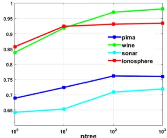
2001) with different parameterhwhich controls the size of feature subsets for each tree on two data sets (musk2 and sonar).Fig. 5 shows how the number of treesntreeaffects the performance of BRFs on the pima, wine, sonar and ionosphere data sets. The curves of the other data sets told a similar story.
FromFig. 4, we can see afterhapproached to 10 all the random forests algorithms lead to satisfactory results for both the ‘‘musk2’’ and ‘‘sonar’’ data sets, which demonstrated that the BRFs algorithm was fairly robust to the parameterh(though the results tend to have small fluctuation).
The obtained classification accuracy results vs. the number of trees in BRFs was shown inFig. 5. We can see that BRFs are basically robust with the number of trees. With the increasing of the number of trees, the classification accuracy increases gradually. When the number of trees is within
[
100,
1000]
, are quite robust. Hence, for simplicity, we chosentree=
100 in our experiments. Moreover, Fig. 5shows that BRFs will not incur over-fitting.7. Conclusion and future work
Random forests play an important role in areas related to ma-chine learning. At present, there are many random forests algo-rithms. Among these forests models, we rarely find one that has both significant practical performance and a complete theoretical guarantee. The structure of the original random forests is mainly based on information theory. However, information theory pays less attention to the intrinsic structure of candidate feature vari-ables. Alternatively, the Banzhaf power index can capture this structure information between feature variables. Motivated by this fact, in this paper, we propose a novel random forests model called Banzhaf random forests (BRFs) and give the proof of its consistency. We have tested BRFs on several UCI data sets and some real world applications. The experimental results demonstrate that BRFs per-form significantly better than existing consistent random forests,
Fig. 5.The performance of BRFs is influenced by the number of treesntreeon four data sets; in this plot, they-axis shows the classification accuracy and the number of trees are shown along thex-axis.
and better than or at least comparable with the original random forests, support vector machines (SVMs) and k-nearest neighbors (KNNs).
Our work is an innovation utilizing the combination of cooper-ative game theory and the random forests algorithm in machine learning. In the future, we will try to combine the game theory and the existing neural networks based on the research results discussed in this paper, so that the neural networks can explore better features for target tasks. In fact, there has already been some studies that combined Game Theory and the neural net-works (Fung & Liu, 2003;Goodfellow, Pouget-Abadie, Mirza, Xu, Warde-Farley, Ozair, Courville, & Bengio, 2014;He, Yu, Huang, Li, & Li, 2014). Typically, Generative Adversarial Networks (GANs) are built upon the two person zero-sum game (two-player game) in the Game Theory. In addition, the efficiency of existing network models can be improved by combining the proposed random for-est algorithm. Moreover, we will try to combine other solution concepts of cooperative game theory (i.e. the Shapley value and the nucleolus) with random forest algorithms or existing neural networks to develop new learning models.
Acknowledgments
This work was supported by the National Key R&D Program of China under Grant No. 2016YFC1401004, the National Natural Science Foundation Of China (NSFC) under Grant No. 61473236 and 61403353, the International Science & Technology Cooperation Program of China (ISTCP) under Grant No. 2014DFA10410, the Science and Technology Program of Qingdao under Grant No. 17-3-3-20-nsh, the Suzhou Science and Technology Program under grant no. SYG201712 and SZS201613, the CERNET Innovation Project under Grant No. NGII20170416, the Key Program Special Fund in XJTLU under Grant No. KSF-A-01, and the Fundamental Research Funds for the Central Universities of China.
References
Amit, Y., & Geman, D. (1997). Shape quantization and recognition with randomized trees.Neural Computation,9(7), 1545–1588.
Amozegar, M., & Khorasani, K. (2016). An ensemble of dynamic neural network identifiers for fault detection and isolation of gas turbine engines.Neural Net-works,76, 106–121.
Ayerdi, B., & Grana, M. (2014). Hybrid extreme rotation forest.Neural Networks,52, 33–42.
Banzhaf III, J. F. (1964). Weighted voting doesn’t work: A mathematical analysis.
Rutgers Law Review,19, 317–343.
Biau, G. (2012). Analysis of a random forests model.Journal of Machine Learning Research (JMLR),13(1), 1063–1095.
Biau, G., Devroye, L., & Lugosi, G. (2008). Consistency of random forests and other averaging classifiers.Journal of Machine Learning Research (JMLR),9, 2015–2033. Bosch, A., Zisserman, A., & Muoz, X. (2007). Image classification using random
forests and ferns. InIEEE conference on computer vision(pp. 1–8). IEEE. Breiman, L. (1996). Bagging predictors.Machine Learning,24(2), 123–140. Breiman, L. (2001). Random forests.Machine Learning,45(1), 5–32.
Breiman, L. (2004). Consistency for a simple model of random forests. Technical report 670.
Breiman, L., Friedman, J., Stone, C. J., & Olshen, R. A. (1984).Classification and regression trees. CRC press. 40(3), 582–588.
Bulo, S. R., & Kontschieder, P. (2014). Neural decision forests for semantic image labelling. InComputer vision and pattern recognition(pp. 81–88).
Chalkiadakis, G., Elkind, E., & Wooldridge, M. (2011). Computational aspects of cooperative game theory.Synthesis Lectures on Artificial Intelligence and Machine Learning,5(6), 1–168.
Chang, C. C., & Lin, C. J. (2007). LIBSVM: a library for support vector machines.ACM Transactions on Intelligent Systems and Technology,2(3), 389–396.
Cormen, T., Leiserson, C., Rivest, R., & Stein, C. (2009).Introduction to algorithms(3rd ed.). The MIT Press.
Criminisi, A., & Shotton, J. (2013).Decision forests for computer vision and medical image analysis. Springer Science & Business Media. 273–293.
Criminisi, A., Shotton, J., & Konukoglu, E. (2012). Decision forests: A unified frame-work for classification, regression, density estimation, manifold learning and semi-supervised learning.Foundations and Trends in Computer Graphics and Vision,7, 81–227.
Cutler, D. R., Edwards Jr., T. C., Beard, K. H., Cutler, A., Hess, K. T., Gibson, J., & Lawler, J. J. (2007). Random forests for classification in ecology.Ecology,88(11), 2783–2792.
Demsar, J. (2006). Statistical comparisons of classifiers over multiple data sets.
Journal of Machine Learning Research (JMLR),7(1), 1–30.
Denil, M., Matheson, D., & De Freitas, N. (2013a). Narrowing the gap: random forests in theory and in practice. InInternational conference on machine learning
(pp. 665–673).
Denil, M., Matheson, D., & de Freitas, N. (2013b). Consistency of online random forests. InInternational conference on machine learning(pp. 1256–1264). Dietterich, T. G. (2000). An experimental comparison of three methods for
con-structing ensembles of decision trees: Bagging, boosting, and randomization.
Machine Learning,40(2), 139–157.
Dollar, P., & Zitnick, C. L. (2014). Fast edge detection using structured forests.IEEE Transactions on Pattern Analysis and Machine Intelligence,37(1), 1558–1570. Feltkamp, V. (1995). Alternative axiomatic characterizations of the Shapley and
Banzhaf values.International Journal of Game Theory,24(2), 179–186. Friedman, J. H. (2001). Greedy function approximation: a gradient boosting
ma-chine.Annals of Statistics, 1189–1232.
Fung, W. K., & Liu, Y. H. (2003). Adaptive categorization of ART networks in robot behavior learning using game-theoretic formulation.Neural Networks,16(10), 1403.
Geurts, P., Ernst, D., & Wehenkel, L. (2006). Extremely randomized trees.Machine Learning,63(1), 3–42.
Goodfellow, I. J., Pouget-Abadie, J., Mirza, M., Xu, B., Warde-Farley, D., Ozair, S., Courville, A., & Bengio, Y. (2014). Generative adversarial networks.Advances in Neural Information Processing Systems,3, 2672–2680.
Györfi, L., Devroye, L., & Lugosi, G. (1996).A probabilistic theory of pattern recognition. Springer-Verlag. 63(279): 194–199.
Hallman, S., & Fowlkes, C. C. (2015). Oriented edge forests for boundary detection. InIEEE conference on computer vision and pattern recognition(pp. 1732–1740). He, X., Yu, J., Huang, T., Li, C., & Li, C. (2014). Neural network for solving nash
equilib-rium problem in application of multiuser power control.Neural Networks,57(9), 73–78.
Ho, T. K. (1998). The random subspace method for constructing decision forests.
IEEE Transactions on Pattern Analysis and Machine Intelligence,20(8), 832–844. Ishwaran, H., & Kogalur, U. B. (2010). Consistency of random survival forests.
Statistics&Probability Letters,80(13), 1056–1064.
Kim, J., Jang, G. J., & Lee, M. (2016). Fast learning method for convolutional neural networks using extreme learning machine and its application to lane detection.
Neural Networks,87, 109–121.
Mcquoid, M. R. J. (1993). Neural ensembles: Simultaneous recognition of multiple 2-D visual objects.Neural Networks,6(7), 907–917.
Meinshausen, N. (2006). Quantile regression forests.Journal of Machine Learning Research (JMLR),7, 983–999.
Pavel, M. S., Schulz, H., & Behnke, S. (2017). Object class segmentation of RGB-D video using recurrent convolutional neural networks.Neural Networks,88, 105–113.
Prasad, A. M., Iverson, L. R., & Liaw, A. (2006). Newer classification and regres-sion tree techniques: bagging and random forests for ecological prediction.
Ecosystems,9(2), 181–199.
Ristin, M., Guillaumin, M., Gall, J., & Van Gool, L. (2016). Incremental learning of random forests for large-scale image classification.IEEE Transactions on Pattern Analysis and Machine Intelligence,38(3), 490–503.
Roy, A., & Todorovic, S. (2016). Monocular depth estimation using neural regression forest. InComputer vision and pattern recognition(pp. 5506–5514).
Saad, W., Han, Z., Debbah, M., & Hjorungnes, A. (2009). Coalitional game theory for communication networks.Signal Processing Magazine IEEE,26(5), 77–97. Salzberg, S. L. (1994). C4.5: programs for machine learning by J. Ross Quinlan.
Morgan kaufmann Publishers, Inc., 1993.Machine Learning,16(3), 235–240. Scardapane, S., & Di, L. P. (2017). A framework for parallel and distributed training
of neural networks.Neural Networks,91, 42–54.
Shotton, J., Johnson, M., & Cipolla, R. (2008). Semantic texton forests for image categorization and segmentation. InIEEE conference on computer vision and pattern recognition(pp. 1–8). IEEE.
Shotton, J., Sharp, T., Kipman, A., Fitzgibbon, A., Finocchio, M., Blake, A., Cook, M., & Moore, R. (2013). Real-time human pose recognition in parts from single depth images.Communications of the ACM,56(1), 116–124.
Svetnik, V., Liaw, A., Tong, C., Culberson, J. C., Sheridan, R. P., & Feuston, B. P. (2003). Random forest: a classification and regression tool for compound classification and qsar modeling.Journal of Chemical Information and Computer Sciences,43(6), 1947–1958.
Yin, P., Criminisi, A., Winn, J., & Essa, M. S. (2007). Tree-based classifiers for bilayer video segmentation. InIEEE conference on computer vision and pattern recogni-tion(pp. 18–23). IEEE.
Zhang, L., & Suganthan, P. N. (2014). Random forests with ensemble of feature spaces.Pattern Recognition,47(10), 3429–3437.
Zikic, D., Glocker, B., & Criminisi, A. (2013). Atlas encoding by randomized forests for efficient label propagation. InMedical image computing and computer-assisted intervention(pp. 66–73). Springer.