with Applications
Scuola di Dottorato in Scienze Statistiche
Dottorato di Ricerca in Statistica Metodologica – XXIX Ciclo
Candidate Francesco Dotto ID number 1179428
Thesis Advisors
Prof. Alessio Farcomeni Prof. Agustín Mayo-Iscar
A thesis submitted in partial fulfillment of the requirements for the degree of Doctor of Philosophy in Statistics
Thesis defended on 21 February 2017
in front of a Board of Examiners composed by: Prof. Caterina Conigliani (chairman)
Prof. Maria Giovanna Ranalli Dr. Pietro Coretto
Advances in Robust Clustering Methods with Applications
Ph.D. thesis. Sapienza – University of Rome © 2016 Francesco Dotto. All rights reserved Author’s email: [email protected]
Contents iv
List of figures ix
List of tables xiii
Introduction 1
1 Robust Statistics: An overview 5
1.1 Contamination: some general notions . . . 5
1.2 Contamination: models . . . 6
1.2.1 Spurious outliers model . . . 6
1.2.2 Tukey-Huber contaminated model . . . 7
1.3 Multivariate Robust Statistics . . . 7
1.3.1 Introduction . . . 7
1.3.2 Multivariate outliers . . . 8
1.3.3 MCD approach . . . 9
1.3.4 Reweighted MCD approach . . . 10
1.3.5 Alternative Approaches . . . 11
1.4 Robust Statistics: some useful tools . . . 12
1.4.1 The influence function and some related quantities . . . 12
1.4.2 The breakdown point . . . 13
2 Robust Clustering Methods 17
Contents vi
2.1 Introduction and state of art . . . 17
2.1.1 Trimmed k-means . . . 18
2.2 Heterogeneus robust clustering based on trimming . . . 19
2.2.1 Formalization of the problem . . . 19
2.2.2 A “naive” extension of the fast MCD algorithm . . . 20
2.2.3 Spurious maximizers . . . 21
2.2.4 Constraint based on the determinant . . . 22
2.2.5 Hathaway-Dennis-Beale-Thompson constraints . . . 23
2.3 The TCLUST methodology . . . 24
2.3.1 Introduction . . . 24
2.3.2 Mathematical formulation . . . 24
2.3.3 The algorithm . . . 25
2.3.4 Open Issues . . . 26
3 Reweighting in Robust Clustering 29 3.1 Introduction . . . 29
3.2 Methodology . . . 30
3.3 The algorithm . . . 33
3.4 Comments on the algorithm . . . 34
3.5 Illustrative examples . . . 35
3.6 Theoretical results . . . 39
3.7 Simulation study . . . 41
4 Extension of TCLUST to fuzzy linear clustering 49 4.1 Introduction . . . 49
4.2 Methodology and algorithm . . . 51
4.2.1 Defining the problem . . . 51
4.2.2 Proposed algorithm . . . 52
4.3 Interpretation and choice of the tuning parameters . . . 55
4.3.2 Number of clusters . . . 56
4.3.3 Fuzzification Parameter . . . 58
4.3.4 Constraints on the residual variances . . . 60
4.3.5 Trimming level . . . 63
4.3.6 Automatically choosing all parameters . . . 63
4.4 Simulation study . . . 65
4.4.1 Settings and methods . . . 65
4.4.2 Automatic choice of the tuning parameters . . . 73
4.4.3 Comments on the results of the simulation study . . . 74
5 Real data examples 79 5.1 Introduction . . . 79
5.2 Applications of reweighted TCLUST . . . 80
5.2.1 Swiss Bank Notes . . . 80
5.2.2 Food Security Data . . . 82
5.3 Applications of fuzzy linear clustering . . . 85
6 Conclusions and further directions 89 6.1 Concluding remarks on the reweighted TCLUST contribution . . . . 89
6.2 Concluding remarks on the TCLUST extension to fuzzy linear clus-tering models . . . 90
6.3 Overall conclusions and further direction of research . . . 91
6.3.1 Preliminary simulation results . . . 93
Appendix A 97 A.1 Proofs of the theoretical properties of the RTCLUST methodology . . 97
A.1.1 Introduction and notation . . . 97
A.1.2 Proof of Theorem 1 . . . 98
A.1.3 Proof of Theorem 2 . . . 99
A.1.4 Proof of Theorem 3 . . . 99
Contents viii
A.2 Justification of Algorithm 6 . . . 102 A.3 A proposal for standardizing the residual component in Algorithm 6 . 104
2.1 Comparison between constrained and unconstrained clustering. . . 22
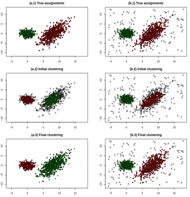
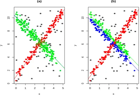
3.1 Two simulated data sets with their true assignments in (a.1) and (b.1). The result of TCLUST withα0 = 0.33 in (a.2) and (b.2). The
final assignments obtained after applying the proposed methodology are given in (a.3) and (b.3). Noisy data and trimmed are denoted by
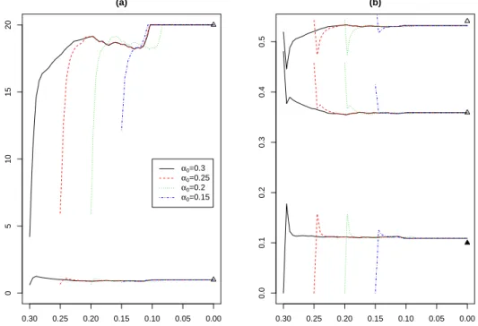
◦ in all graphs throughout the manuscript. . . 32 3.2 Evolution of |Σlj| in (a) and ofπjl in (b) for different initial α0 values
(α0 =.3, .25, .2 and .15) for the data set shown in Figure 3.1 (b.1).
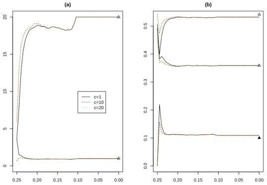
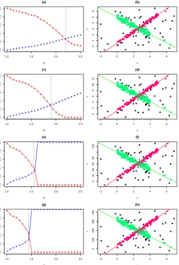
The up-triangle symbols are the true parameters to be estimated. . . 36 3.3 Evolution of |Σlj| in (a) and of πlj in (b) for different initial c values
(c = 1, 10 and 20 while the true c needed was 11.71) for the data set shown in Figure 3.1 (b.1). The up-triangle symbols are the true parameters to be estimated. . . 37 3.4 (a) The proposed iterative reweighting procedure whenk = 1 started
from α0 = 0 and αL = 0.01 (b) The (traditional) reweighted MCD
started from α0 = 0 and αL = 0.01. Trimmed points are the black
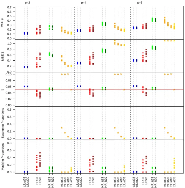
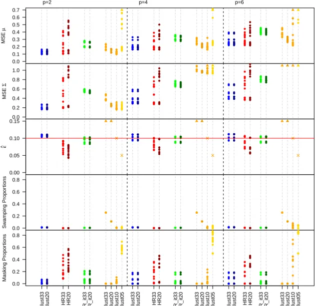
points. . . 38 3.5 Results when ε = 0.05. Every procedure is labeled as explained in
the text. Values appearing in the Figure that are fixed in advance (e.g the trimming level for the tclust method) are plotted with the symbol “×” while when the considered value exceeds the scale of the plot we used a “4” . . . 45 3.6 Results when ε = 0.10. Every procedure is labeled as explained in
the text. . . 46 3.7 Simulation results study under no contamination (ε= 0). . . 47
List of figures x
4.1 (a) Robust fuzzy clustering results whenk = 3 andpj are used within
the objective function. (b) Results when k = 3 and pj are not used
within the objective function. . . 57 4.2 (a) A simulated dataset with two overlapped linear clusters and 10%
of contaminated points. (b) The associated “classification trimmed likelihood curves” whenc= 5 andm= 1.5. . . 58 4.3 Different degrees of fuzzification obtained for different scale values s
(yi is replaced by yi ·s). m = 1.5 and s = 0.5 in (a); s = 1 in (c);
s = 10 in (e); s = 32 in (g). m = 1 (hard clustering) and s= 0.5 in (b); s= 1 in (d); s= 10 in (f); s= 32 in (h). . . 59 4.4 Left panels: relative entropy of the fuzzy weights, “×”, proportion of
hard assignments, “◦”, as a function of scale; (a) s = 0.5. (c) s = 1 (e) s = 10. (g) s= 32. Right panels: clustering obtained for specific values of m through (b) s = 0.5, m = 2.2. (d) s = 1, m = 1.8. (f)
s= 10, m= 1.6. (h)s = 32,m = 1.4. . . 61 4.5 Estimated robust fuzzy clustering for different c values in two (less
and more) heteroscedastic data sets. c= 5 is used in (a) and (d) and
c= 1 in (b) and (d). The plotted bands are obtained by adding±2bsj
to each fitted regression line. . . 62 4.6 (a) FTCR withc= 5 andk = 2. (b) FTCR withc= 1010and k = 2.
(c) FTCR with c= 1010 and k = 3. . . 62
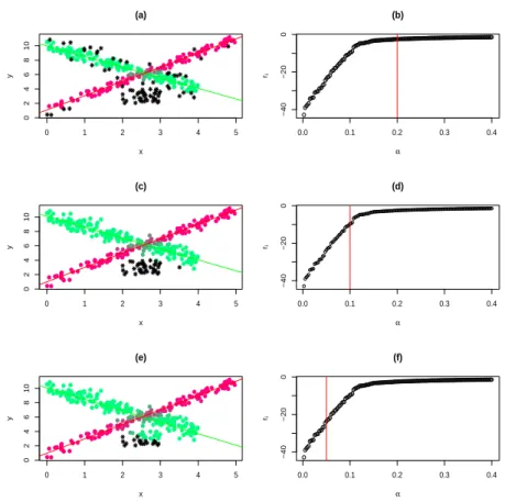
4.7 Left panels: Estimated linear clustering result for different trimming levels and m = 1.5. (a) α = 0.20. (c) α = 0.10. (e) α = 0.05. Right panels: Average contribution to the likelihood for different val-ues of α. A red line corresponds to the trimming level used on the corresponding left panel. (b): α= 0.20. (d): α= 0.10. (f): α= 0.05. 64 4.8 (a) The scatter plot of our dataset. (b) The results obtained using
the tuning parameters chosen by cross-validation . . . 65 4.9 Simulation study. Boxplots representing the MSE ofbj and b0j for
set-ting S1: p= 1,k = 2. The Homoscedastic clusters are in (a),(c),(e),(g). Heteroscedastic clusters are in (b), (d), (f), (h). Uniform contami-nation is in (a) and (b). Inflated uniform contamicontami-nation is in (c), and(d). Pointwise contamination in (e) and (f). Clean dataset is in (g) and (h) . . . 67
4.10 Simulation study. Misclassification error for setting S1: p= 1, k = 2. Legend as in Figure 4.9. . . 68 4.11 Simulation study. Boxplots representing the MSE of bj and b0j for
setting S2: p= 2, k= 2. Same legend of Figure 4.9. . . 69 4.12 Simulation study. Misclassification error for setting S2: p= 2, k = 2.
Legend as in Figure 4.9 . . . 70 4.13 Simulation study. Boxplots representing the MSE of bj and b0j for
setting S3: p= 4, k= 2. Same legend of Figure 4.9 . . . 71 4.14 Simulation study. Misclassification error for setting S2: p= 2, k = 2.
Legend as in Figure 4.9 . . . 72 4.15 Simulation study. Boxplots representing the MSE of bj and b0j for
setting S4: p= 1, k= 3. Legend as in Figure 4.9 . . . 73 4.16 Simulation study. Misclassification error for setting S4: p= 1, k = 3.
Legend as in Figure 4.9 . . . 74 4.17 Simulation study. Boxplots representing the MSE of bj and b0j for
setting S5: p= 2, k= 3. Legend as in Figure 4.9 . . . 75 4.18 Simulation study. Misclassification error for setting S5: p= 2, k = 3.
Legend as in Figure 4.9 . . . 75 4.19 Simulation study. Boxplots representing the MSE of bj and b0j for
setting S6: p= 4, k= 3. Same legend of Figure 4.9 . . . 76 4.20 Simulation study. Misclassification error for setting S6: p= 4, k = 3.
Legend as in Figure 4.9. . . 76 4.21 Boxplots with Mean Square Error for tuned and crossvalidated model,
with competitors for comparison. C-val denotes FTCR with auto-matically chosen tuning. (a) Two Homoscedastic clusters uniformly contaminated,p= 1 covariate (Setting S1). (b) Two Heteroscedastic clusters with pointwise contamination,p= 1 covariate (Setting S1). . 77
5.1 Fourth against the sixth variable of the Swiss Bank Notes data set. (a) G stands for genuine bills, F for forged ones and 15 bills listed
in Flury & Riedwyl (1988) as anomalous ones are surrounded by ◦
symbols. (b) The initial TCLUST solution with α0 = 0.33 (c) Final
solution when applying the proposed iterative approach. Trimmed observations not coinciding with those in Flury and Riedwyl’s list are surrounded by 2 symbols. . . 81
List of figures xii
5.2 ctlcurveplot for the FIES data. . . 83
5.3 Pinus Nigra example. (a) ctlcurve. (b) average contribution to the
likelihood as a function ofα. (c) relative empty entropy and propor-tion of hard assignments as a funcpropor-tion ofm. . . 86
5.4 Pinus Nigra example: (a) Scatter plot and results of cReg method.
(b) results of the “EM” method. (c) results of the A-cReg method. (d) results of the FTCR method. Circled observations are fuzzy as-signments. . . 87
5.5 Pinus Nigra Data example: Results of the proposed procedure when
searching fork = 4 clusters and no trimming imposed . . . 88
A.1 Empirical Comparison of the impact of the scale of the data as before and after the standardization (A.7) . . . 105
5.1 99% simultaneous confidence intervals for ˆµprovided by the TCLUST and the RTCLUST . . . 81 5.2 Cluster profiles and measurements for the outlying countries. FIES:
Food Insecurity Experience Scale. CE: Civic Engagement. St: Strug-gling. FS: Food Security. Co: Corruption index. YD: Youth Devel-opment. C-j: j-th cluster profile. . . 84
6.1 List of 10 different models obtained by imposing different constraint in decomposition (6.1) . . . 92 6.2 Simulation results based on B=500 replicates: average MSE of the
estimated vector mean in each cluster . . . 95
Robust methods in statistics are mainly concerned with deviations from model as-sumptions. As already pointed out in Huber (1981) and in Huber & Ronchetti
(2009) “these assumptions are not exactly true since they are just a mathematically convenient rationalization of an often fuzzy knowledge or belief”. For that reason “a minor error in the mathematical model should cause only a small error in the final conclusions”. Nevertheless it is well known that many classical statistical procedures are “excessively sensitive to seemingly minor deviations from the assumptions”. All statistical methods based on the minimization of the average square loss may suffer of lack of robustness. Illustrative examples of how outliers’ influence may completely alter the final results in regression analysis and linear model context are provided in Atkinson & Riani(2012). A presentation of classical multivariate tools’ robust counterparts is provided in Farcomeni & Greco (2015).
The whole dissertation is focused on robust clustering models and the outline of the thesis is as follows.
Chapter 1 is focused on robust methods. Robust methods are aimed at increasing the efficiency when contamination appears in the sample. Thus a general definition of such (quite general) concept is required. To do so we give a brief account of some kinds of contamination we can encounter in real data applications. Secondly we introduce the “Spurious outliers model” (Gallegos & Ritter 2009a) which is the cornerstone of the robust model based clustering models. Such model is aimed at formalizing clustering problems when one has to deal with contaminated samples. The assumption standing behind the “Spurious outliers model” is that two differ-ent random mechanisms generate the data: one is assumed to generate the “clean” part while the another one generates the contamination. This idea is actually very common within robust models like the “Tukey-Huber model” which is introduced in Subsection 1.2.2. Outliers’ recognition, especially in the multivariate case, plays a key role and is not straightforward as the dimensionality of the data increases. An overview of the most widely used (robust) methods for outliers detection is provided within Section 1.3. Finally, in Section 1.4, we provide a non technical review of the classical tools introduced in the Robust Statistics’ literature aimed at evaluating the
2
robustness properties of a methodology.
Chapter 2 is focused on model based clustering methods and their robustness’ prop-erties.
Cluster analysis, “the art of finding groups in the data” (Kaufman & Rousseeuw 1990), is one of the most widely used tools within the unsupervised learning context. A very popular method is the k-means algorithm (MacQueen et al. 1967) which is based on minimizing the Euclidean distance of each observation from the estimated clusters’ centroids and therefore it is affected by lack of robustness. Indeed even a single outlying observation may completely alter centroids’ estimation and simulta-neously provoke a bias in the standard errors’ estimation. Cluster’s contours may be inflated and the “real” underlying clusterwise structure might be completely hidden. A first attempt of robustifying thek- means algorithm appeared inCuesta-Albertos
et al. (1997), where a trimming step is inserted in the algorithm in order to avoid
the outliers’ exceeding influence.
It shall be noticed that k-means algorithm is efficient for detecting spherical ho-moscedastic clusters. Whenever more flexible shapes are desired the procedure be-comes inefficient. In order to overcome this problem Gaussian model based cluster-ing methods should be adopted instead of k-means algorithm. An example, among the other proposals described in Chapter 2, is the TCLUST methodology (
Garc´ıa-Escudero et al. 2008), which is the cornerstone of the thesis. Such methodology is
based on two main characteristics: trimming a fixedproportion of observations and imposing a constraint on the estimates of the scatter matrices. As it will be ex-plained in Chapter 2, trimming is used to protect the results from outliers’ influence while the constraint is involved as spurious maximizers may completely spoil the solution.
Chapter 3 and 4 are mainly focused on extending the TCLUST methodology. In particular, in Chapter 3, we introduce a new contribution (compare Dotto et al.
2015 and Dotto et al. 2016b), based on the TCLUST approach, called reweighted
TCLUST or RTCLUST for the sake of brevity. The idea standing behind such method is based on reweighting the observations initially flagged as outlying. This is helpful both to gain efficiency in the parameters’ estimation process and to pro-vide a reliable estimation of the true contamination level. Indeed, as the TCLUST is based on trimming a fixed proportion of observations, a proper choice of the trimming level is required. Such choice, especially in the applications, can be cum-bersome. As it will be clarified later on, RTCLUST methodology allows the user to overcome such problem. Indeed, in the RTCLUST approach the user is only required to impose a high preventive trimming level. The procedure, by iterating through a sequence of decreasing trimming levels, is aimed at reinserting the discarded obser-vations at each step and provides more precise estimation of the parameters and a
final estimation of the true contamination level ˆα.
The theoretical properties of the methodology are studied in Section 3.6 and proved in Appendix A.1, while, Section 3.7, contains a simulation study aimed at evaluating the properties of the methodology and the advantages with respect to some other robust (reweigthed and single step procedures).
Chapter 4 contains an extension of the TCLUST method for fuzzy linear cluster-ing (Dotto et al. 2016a). Such contribution can be viewed as the extension of
Fritz et al. (2013a) for linear clustering problems, or, equivalently, as the
exten-sion of Garc´ıa-Escudero, Gordaliza, Mayo-Iscar & San Mart´ın (2010) to the fuzzy clustering framework. Fuzzy clustering is also useful to deal with contamination. Fuzziness is introduced to deal with overlapping between clusters and the presence
of bridge points, to be defined in Section 1.1. Indeedbridge points may arise in case
of overlapping between clusters and may completely alter the estimated cluster’s parameters (i.e. the coefficients of a linear model in each cluster). By introducing fuzziness such observations are suitably down weighted and the clusterwise struc-ture can be correctly detected. On the other hand, robustness againstgross outliers, as in the TCLUST methodology, is guaranteed by trimming a fixed proportion of observations. Additionally a simulation study, aimed at comparing the proposed methodology with other proposals (both robust and non robust) is also provided in Section 4.4.
Chapter 5 is entirely dedicated to real data applications of the proposed contribu-tions. In particular, the RTCLUST method is applied to two different datasets. The first one is the “Swiss Bank Note” dataset, a well known benchmark dataset for clus-tering models, and to a dataset collected by Gallup Organization, which is, to our knowledge, an original dataset, on which no other existing proposals have been ap-plied yet. Section 5.3 contains an application of our fuzzy linear clustering proposal to allometry data. In our opinion such dataset, already considered in the robust linear clustering proposal appeared in Garc´ıa-Escudero, Gordaliza, Mayo-Iscar &
San Mart´ın (2010), is particularly useful to show the advantages of our proposed
methodology. Indeed allometric quantities are often linked by a linear relationship but, at the same time, there may be overlap between different groups and outliers may often appear due to errors in data registration.
Finally Chapter 6 contains the concluding remarks and the further directions of research. In particular we wish to mention an ongoing work (Dotto & Farcomeni,
In preparation) in which we consider the possibility of implementing robust
parsi-monious Gaussian clustering models. Within the chapter, the algorithm is briefly described and some illustrative examples are also provided. The potential advan-tages of such proposals are the following. First of all, by considering the parsimo-nious models introduced in Celeux & Govaert(1995), the user is able to impose the
4
shape of the detected clusters, which often, in the applications, plays a key role. Secondly, by constraining the shape of the detected clusters, the constraint on the eigenvalue ratio can be avoided. This leads to the removal of a tuning parameter of the procedure and, at the same time, allows the user to obtain affine equivariant esti-mators. Finally, since the possibility of trimming a fixed proportion of observations is allowed, then the procedure is also formally robust.
Robust Statistics: An overview
1.1
Contamination: some general notions
As briefly stated in the introduction, robust methods aim to provide methodologies which are resistant with respect to mild deviations from the assumed parametric model. This implies that in the observed sample there are points which do not follow the underlying distribution, that is to say, contaminating points or outliers. Contamination is a very general notion that may be defined in different ways de-pending on the context of application. Following Farcomeni & Greco (2015) we try here to give a non-exhaustive account of some types of contamination that are likely to be found in data analysis:
• Extreme values orgross outliers. Points unusually large (or small) with respect
to one or more dimensions
• Influential outliers or leverage points. Points that do not follow the pattern
shown by the majority of the data (i.e. points presenting negative correlation between two dimensions when data exhibit positive one)
• Inliers. Corrupted points that lie very close to the sample mean deflating the
variance.
• Bridge points. Points lying very close to the boundaries of two clusters. These
points play a key role in cluster analysis. Indeed bridge points may be very difficult to assign to one cluster and can be dangerous for parameters’ estima-tion.
Generally speaking robust procedures are designed in order to be efficient in cases where contamination appears in the sample. As it will be clarified in the further
1.2 Contamination: models 6
chapters, impartial trimming (Garc´ıa-Escudero et al. 2008) is a useful tool in order to deal with contaminating points.
It must be pointed out that trimming is supposed to discard the “farthest” values from the clusters’ centers. In case of overlap between clusters, bridge points may appear in the sample and trimming may not work well. Thus a different framework will be considered in Chapter 4. In particular we will consider the case of fuzzy
partitions, instead of hard partitions. Considering hard partitions in clustering is equivalent to assign a binary weight to the i-th observation uij ∈ {0,1} and uij = 1
if and only if observation i belongs to cluster j. On the other hand, in case of fuzzy partitions uij ∈ [0,1]. Thus, within the fuzzy framework, each observation is
simultaneously assigned to more than one cluster and the degree of membership of observation i to each cluster j is given by its fuzzy weight uij.
1.2
Contamination: models
Robust methods aim to contain the exceeding influence of the outlying points. To do so, the sample is generally supposed to come from two different probability density functions: one generating the “clean part” of the data, and the other one, generally called contaminating density, generating the contaminated part of the sample. In-deed, especially within the multivariate context, identifying the contaminated part of the data is necessary to be able to contain its influence by treating it in a different way (e.g by trimming or downweighting).
1.2.1
Spurious outliers model
One of the most widely used models suitable for cluster analysis is the “spurious outliers model”, introduced in Gallegos & Ritter (2005). Such model keeps in ac-count the presence of two different densities: one is a mixture made ofkcomponents, where each component of the mixture generates each cluster, and the other is a con-taminating density, which generated the outlying component of the data. A more detailed definition follows.
Definition 1. Letxi ∈Rp be a sample point,f(·) the multivariate normal density,
µj and Σj be location and scatter parameters, respectively, of thej-th group.
Addi-tionally let gψi(·) be the contaminating density and K the number of groups. Then
the likelihood function associated to the spurious outliers model is given by:
" K Y j=1 Y i∈Rj f(xi;µj; Σj) #" Y i /∈Rj gψi(xi) # (1.1)
Additionally it must be pointed out that, in equation (1.1), R =SK
j=1Rj
repre-sents the set of the clean observation and is such that #R =dn(1−α)e. As it will be clarified in the further sections, only the clean data give a contribution to the likelihood function, while, outliers give no contribution to function (1.1).
1.2.2
Tukey-Huber contaminated model
Spurious outliers model is an adaptation of the Tukey-Huber contamination1 model
(Tukey 1962 and Huber et al. 1964), which is defined as follows.
Definition 2. Let F be the model generating the data, generally assumed to be Gaussian throughout the whole dissertation, G the contaminating model and
ε the proportion of observation arising from the contaminating model. The ε -neighborhood or Tukey-Huber contaminated model is defined as:
P(F, ε) = {Fε|Fε = (1−ε)F(X;θ) +εG(X), θ ∈Θ, X ∈ X } (1.2)
Generally speaking the more a statistics (output of a procedure)T(F) is resistant to contamination, the more is considered as robust.
Definitions 1 and 2 provide a very general formalization of the concept of con-taminated models. Throughout this dissertation, whenever we refer to concon-taminated data, we implicitly refer to a data generating mechanism outlined either in Definition 1 or in Definition 2.
1.3
Multivariate Robust Statistics
1.3.1
Introduction
Given a multivariate sample X = (x1, . . . , xn) with xi ∈ Rp and p≥ 1, the sample
mean vector, ˆµ, and the sample covariance matrix, ˆΣ, are standard tools for de-scribing location, variability and pairwise dependence in the data. Usage of such quantities is also motivated by the fact that these are the MLE estimators of the location and scale parameters at the multivariate Gaussian model. It shall be no-ticed that the multinormal distributional assumption of the data is pretty common although it may be too restrictive in some cases.
As in the univariate case, such quantities suffer of lack of robustness since even one single observation may completely spoil the yielding estimates. Illustrative exam-ples may be encountered, among the others, inGarc´ıa-Escudero et al. (2012). Thus
1.3 Multivariate Robust Statistics 8
the influence of outlying points needs to be controlled although, as the dimension-ality of the data increases, outliers’ identification becomes an hard task. Indeed, as visualization’s tools can not be applied, alternative methods are required.
1.3.2
Multivariate outliers
Let us suppose, that xi ∼ N(µ,Σ) where xi ∈ Rp and N(µ,Σ) stands for the
multivariate normal distribution with location parameter µ and scale parameter Σ. Generally speaking outliers are observation placed “far” from the bulk of the data. For that reason suitable methods for defining the distance from the bulk of the data are required. Clearly the usage of the simple Euclidean distance from a suitably defined center of the data is not enough since such value is affected by the scale. The most commonly used distance measure in multivariate statistics is the Mahalanobis distance:
dΣ(xi, µ) =
p
(xi−µ)TΣ−1(xi−µ) (1.3)
where in equation (1.3) xi ∈ Rp is a sample point, µ ∈ Rp is a location parameter
and Σ ∈P D(Mpxp) is a scale parameter. It easy to note that if Σ = I
pxp then the
Mahalanobis distance is equivalent to the Euclidean distance while, on the other hand, as p= 1 the Mahalanobis distance reduces to the well known z-score. Maha-lanobis distance evaluation plays a key role in multivariate outliers’ detection: every observation exceeding a pre-fixed value of the Mahalanobis distance may be flagged as outlying. In order to fix this value one may refer to the asymptotic distribution of the Mahalanobis distance which can be approximated:
d2Σ(xi;µ)∼χ2p (1.4)
Clearly formula (1.4) provides a very “naive” approximation and the true param-eters of the distribution are supposed to be known. In order to improve (1.4),
Gnanadesikan & Kettenring (1972) proposed an exact distribution for the
Maha-lanobis distance as the MLE is plugged in instead of the true parameters’ values:
d2S¯(xi; ¯x)∼ (n−1)2 n Beta p 2, n−p−1 2 ! (1.5)
Typical choices for cut off values are.975 or.99 that correspond to flagging as outly-ing observation out of the boundaries of the 97.5% or 99% of the tolerance ellipsoid. Clearly neither approximation (1.4) nor approximation (1.5) are efficient under con-tamination. Indeed even one single outlier may completely alter the estimation of ¯
swamping ormasking effects. Swampingoccurs when clean observations are flagged as outlying. Such undesired effect may be caused by a deflation of |Σˆ| which may lead to wrongly consider many observations “too far” from the center of the data and thus, flagging them as outlying. On the contrary, as |Σˆ| is overestimated, out-liers may not be recognized and then masking occurs.
For these reasons, some robust counterparts of the classical methods are required.
1.3.3
MCD approach
In order to protect the estimators from the influence of the “farthest” points,
Rousseeuw (1985) proposed to estimate the parameters using a subset containing
only the bulk of the data. The bulk of the data can be recognized as the subsam-ple containing the n(1−α) data points which yield the covariance matrix having the minimum determinant. Once the subset containing the data with the mini-mum determinant of the covariance matrix is identified, then the population mean is estimated straightforwardly by using the sample mean of these points; while the covariance matrix is estimated by multiplying the sample variance of these points for a constant which guarantees the consistency of the estimator. More formally, let α be the fixed proportion discarded and let zi be a binary vector such that
P
zi =n·(1−α). The MCD estimators are defined as:
ˆ µM CD = 1 P izi n X i=1 zixi (1.6) ˆ ΣM CD = c(p, α) P izi−1 n X i=1 (xi−µˆM CD)(xi −µˆM CD)Tzi (1.7)
where the constant term in equation (1.7) is a factor which makes the MCD consis-tent at the Normal model by inflating the estimated covariance matrix. Its explicit formula is the following:
c(p, α) = 1−α
Fχ2
p+2(qp,1−α)
(1.8) More theoretical details on this argument can be found in Liu et al. (1999).
The most popular algorithm for the MCD is the FASTMCD algorithm, proposed in
Rousseeuw & van Driessen (1999), which iterates the following steps:
Algorithm 1.
1. Let ˆθ0 = (ˆµ0,Σˆ0) an initial estimate of the parameters obtained by sampling
1.3 Multivariate Robust Statistics 10
2. Calculate the robust distances d0i =d(xi,θˆ0)
3. Sort the distances in non increasing order and take the subset of size n·(1−α) having the lowest values
4. Update the estimate of the parameter ˆθ1 = (ˆµ1,Σˆ1)
5. Iterate steps 2-4 up to convergence
It is straightforward to see that at each iteration of the algorithm the determinant of the estimated scatter matrix decreases, since, at each step, the observations “clos-est” to each other are inserted in the subsample. By initializing the algorithm from different starting points the global optimum for the objective function (the deter-minant of the scatter matrix) is more likely to be reached. Usually the algorithm is implemented by initializing it 500 times and typical values for α are either 0.25 or 0.50.
Despite computational issues, the MCD algorithm is one of the most widely used approaches to provide robust estimates in a multivariate context; additionally there are interesting asymptotic properties (Butler et al. 1993, in Croux & Haesbroeck
1999 and Cator et al. 2012). From the robustness’ point of view it can be shown
that the asymptotic breakdown point (to be better defined in the further sections) is often equal to the chosen trimming rate. As it will be clarified later on, the maxi-mum value for the breakdown point that can be reached by an estimator is 0.5 which implies that, if α= 0.5, then the MCD estimator is the affine equivariant estimator having the highest possible value for the asymptotic breakdown point.
1.3.4
Reweighted MCD approach
Robustness may cause loss of efficiency since part of the observations are generally discarded. Indeed as α is fixed too high, then too many observations are discarded, provoking a loss of efficiency in the parameter estimation. For that reason, the MCD estimator may be reweighted to increase of efficiency. This leads to a new estimator: the reweighted MCD, usually called RMCD. The reweighting process works as follows:
Algorithm 2.
1. For each i = 1, . . . , n compute the distances di = dΣˆM CD(xi,µˆM CD) from the
MCD estimators defined in (1.6) and (1.7)
3. Update the estimation using formulas (1.6) and (1.7) to update the estimates. A common choice for fixing the threshold to be used in the step 1 of Algorithm 2 is the α0 quantile of the χ2
p distribution. Alternatively a better approximation is
provided in Hardin & Rocke(2004) where a scaled F distribution is proposed:
d2Σˆ
M CD(xi; ˆµM CD)∼
pm
(m−p−1)Fp,m−p+1 (1.9) In equation (1.9)mis a constant whose expression can be found inHardin & Rocke
(2005). It shall be pointed out that approximation (1.9) is optimal for MCD esti-mators, while an suitable approximation for RMCD estiesti-mators, provided in Cerioli
(2010), is given by: d2Σˆ RM CD(xi; ˆµRM CD)∼ (P zi−1)2 P zi Beta p 2, P zi−p−1 2 ! (1.10)
1.3.5
Alternative Approaches
Another popular robust estimator has been proposed in Rousseeuw (1984) and in
Rousseeuw(1985) where the Minimum Volume Ellipsoid (MVE) estimator has been
introduced. Operatively speaking, the MVE estimator looks for the ellipsoid of the minimum volume that contains n(1−α) observations. It shall be noticed that the idea of this estimator is pretty similar to the idea standing behind the MCD estima-tors. An algorithmic method for computing the minimum volume ellipsoid has been proposed Van Aelst & Rousseeuw (2009). Nevertheless, due to the efficiency of the fast MCD algorithm (Algorithm 1), this last estimator has become much more pop-ular than the MVE estimator so far. MCD and MVE are based on hard rejection rules, following the “impartial trimming principle”, explained in Garc´ıa-Escudero
et al. (2008) and in Cuesta-Albertos et al.(2008a). Another method based on
trim-ming is the forward search approach, Atkinson et al. (2004) and Atkinson et al.
(2004), which is based on the idea of starting from a subset of clean observations and iteratively looking for the best sets of increasing size based on the estimates at the previous steps.
Alternative robust approaches are mainly based on underweighting outlying obser-vations instead of trimming them. Among the others, we recall methodologies in
Donoho(1982) andStahel(1981), where the idea is to assign a weight to each
obser-vation depending on its “outlyingness” measured by using a univariate projection of each observation. To our knowledge, an application of these methodologies for clustering has not been proposed yet.
1.4 Robust Statistics: some useful tools 12
1.4
Robust Statistics: some useful tools
A brief review of how to evaluate the robustness of a procedure follows. It must be pointed out that some tools require technical arguments and a direct usage within the robust clustering context is not straightforward. These concepts will be briefly mentioned within this chapter and recalled, as required, along the whole thesis.
1.4.1
The influence function and some related quantities
Influence function: definition
In order to describe the effect of the departure from the assumed model F within a neighborhood Hampel (1974) and Huber (1981) introduced the idea of influence
function. From a mathematical point of view the influence function is defined as
the Gateaux derivative of the functional T(F), with F ∈ F along the direction of
x. More precisely:
Definition 3. LetFε = (1−ε)F +εδx whereδx is Dirac delta random variable
de-generate inx. The influence function for an infinitesimal point mass contamination
ε, at location x, at the model F, is given by:
IF(x;T, F) = lim ε→0 T(Fε)−T(F) ε = ∂ ∂εT(Fε)|ε=0 (1.11)
The influence function provides a global overview of the robustness properties of an estimator as Gateaux derivative’s computation at location x aims at measuring the effect that a contaminating point xmay have on an estimator T(F). Whenever such effect is bounded we its yields that its influence function is bounded as well and the estimator can be considered robust. As an illustrative example let us consider the univariate standard Gaussian model. Let us also consider the sample mean and the sample median as estimators of the location parameter. Their influence function is given, respectively, by:
IF(x; ˆµ,Φ) = x (1.12)
IF(x;M ed,Φ) =
r
π
2sign(x) (1.13) It is clear from equations (1.12) and (1.13) that the influence function associated to the sample mean is unbounded while it becomes bounded in the case of the median. This reflects the well known properties of such estimators. Indeed the influence that a single point may have on the sample mean estimator is unbounded, while, in the case of the median, the estimator moves in the direction of the outlier in a bounded way.
The gross error sensitivity
As briefly stated in the previous paragraph, evaluation of the boundedness of the influence function of an estimator is pretty important in order to assess its robustness properties. Mathematically speaking, the boundedness of the influence function is evaluated by computing the gross error sensitivity, defined as the upper bound of the influence function:
γ∗ = sup
x∈Rp
||IF(x;T, F)|| (1.14) Equation (1.14) allows to measure the highest influence that a fixed size contami-nation may have on the value of an estimator. A bounded value of γ∗ implies that an estimator is influenced in a “bounded” way by any type of contamination. It is indeed a very important property from the robustness point of view and, as a re-sult, estimators having bounded values of γ∗ are formally robust. They are usually referred to B (bias) - robust estimators.
Local shift sensitivity
Data are often slightly changed (due to inaccuracies in data registration or to opera-tions like rounding), and in terms of robustness it is interesting to measure the effect that such changes may have on the chosen estimator. We recall here the definition
of local shift sensitivity given by:
λ∗ = sup
x6=y;x,y,∈Rp
||IF(x;T, F)−IF(y;T, F)||
||x−y|| (1.15)
Equation (1.15) describes the effect of shifting an observation x to a close point y. It is straightforward to see that as y = x+ε with ε → 0 we go back to equation (1.11).
1.4.2
The breakdown point
Introduction
The notion of breakdown point is related with the proportion of observations that can be arbitrarily replaced until an estimator (an output of a procedure) breaks down. Roughly speaking, the higher is the breakdown point, the higher is the ro-bustness of the given procedure. Formal definition of such concept depends strictly on the application of interest. There follow some very general definitions of break-down point and the formalization proposed in Gallegos & Ritter (2009a) which is suitable to evaluate the robustness of a clustering method.
1.4 Robust Statistics: some useful tools 14
Finite sample breakdown point and its generalizations
The finite sample breakdown point, also known asindividual breakdown point(Ruwet
et al. 2013), provides a data dependent definition of the concept of the breakdown
point associated to a given dataset.
Definition 4. Let Xr ∈ Xr where Xr is the collection of all datasets Xr of size
having (n −r) elements in common with the original data Xn. The finite sample
breakdown point is defined as:
εi = max ( r n : supXr ||T(X)−T(Xr)|| ∈K ) (1.16)
where a K is a bounded and closed set that does not contain the boundary points of the parameter space.
In order to overcome the dependency from the data Donoho & Huber (1983) introduced the notion of universal breakdown point.
Definition 5. Let D be the set of all datasets Xn ∈ Rp in general position. The
universal breakdown point is defined as:
ε(u) = max
Xn∈D
ε(i) (1.17)
It shall be noticed that Definition 5 generalizes Definition 4 since the class con-taining all the dataset Xn ∈ Rp is considered in computing the breakdown point
instead of considering a single datasetXn.
Restricted breakdown point
As noticed inRuwet et al.(2013), according to Definitions 4 and 5, a set of estimators obtained by a clustering model may have 0 value for the breakdown point despite their robustness. Indeed “some datasets can hardly be clustered ink clusters simply because the do not come from a k-component model and this makes any clustering method have a 0 value for the universal breakdown point” (Ruwet et al. 2013). For that reason, Gallegos & Ritter (2005) introduced the notion ofrestricted breakdown
point with respect to some subclass K ⊂ D of admissible datasets. In particular,
within cluster analysis, the condition of “well clustered” datasets, proposed in the reference above, is kept in account. The restricted breakdown point is defined as follows.
Definition 6. LetD be the set of all datasets Xn ∈Rp in general position and let
K be a subset of D containing the datasets for which condition of “well clustered” data holds. Then the restricted breakdown point is defined as
ε(r)= max
Xn∈K
ε(i) (1.18)
Definition 6 is generally the one adopted to assess the robustness of a clustering model. Compare as an example Ruwet et al. (2013) where an explicit computation of the tclust method is provided.
More details may be encountered, besides the reference provided so far, inHuber
(1981), inHuber & Ronchetti(2009), where the dissertation on the breakdown point has been hugely extended, and in Ruckdeschel & Horbenko(2012).
Robust Clustering Methods
2.1
Introduction and state of art
Generally speaking “clusters may be thought as regions of high density separated from other such regions by regions of low density”(Hartigan 1975). Cluster anal-ysis aims to identify a prefixed number of clusters within a given dataset. To do so, observations are usually grouped around suitably defined centroids following the aim of maximizing the heterogeneity between the groups and minimizing the homo-geneity within the groups. Clusters’ centroids are either observations or quantities, computed on clusters’ observations, somehow representative of the whole cluster. Detailed reviews on clustering methods are provided, among the others, inAtkinson
& Riani (2012) and in Hennig et al. (2015), or in Farcomeni & Greco (2015) and
in Ritter (2014) for robust methods. Additionally alternative approaches based on
grouping around different types of structures have been proposed so far, as a dif-ferent notion of cluster may be of interest. In particular, one may be interested in clustering around linear structures or other type of manifolds as in Garc´ıa-Escudero
et al. (2009), in Garc´ıa-Escudero, Gordaliza, Mayo-Iscar & San Mart´ın(2010) and
in Hennig (2003).
Among the different approaches to cluster analysis we may distinguish between
distance based methods and model based methods. In the latter approach the
as-sumption of an underlying population model is needed. In our opinion the latter approach has many advantages for mainly two reasons: first more flexible clusters’ shapes are allowed. Secondly, as we are referring to a specified (and flexible as pos-sible) statistical model, further inferential properties of the clustering method can be studied and assessed. Finally it must be pointed out that many distance based
prob-2.1 Introduction and state of art 18
abilistic assumptions. As an example consider the k-means algorithm (MacQueen
et al. 1967). This clustering method aims to minimize the Euclidean distance from
k centroids which corresponds, from a probabilistic point of view, to assume that the data arise from k spherical homoscedastic multinormal populations. As in the case of the k means, oftentimes probabilistic assumptions are implicitly done even in cases where an underlying model is not properly formalized.
The outline of the chapter is as follows. Firstly we introduce the most relevant con-tributions related with robust clustering models. We start from thek-means’ robust counterpart, the trimmed k-means (Cuesta-Albertos et al. 1997), and then, in sec-tion 2.2, we introduce more sophisticated methods which are able to deal with data divided in heterogeneous clusters. In section 2.3, we present the tclust method
(Garc´ıa-Escudero et al. 2008) and the open issues related with this methodology.
2.1.1
Trimmed
k
-means
One of the most widely adopted approach for cluster analysis is the k-means al-gorithm. Given a sample {x1, . . . , xn} with xi ∈ Rp, k-means algorithm aims to
minimize the following quantity: inf m1,...,mk∈Rp n X i=1 min j=1,...,k||xi−mj|| 2 (2.1)
It shall be noticed that the optimization problem introduced in formula (2.1) is based on minimizing a least square criterium and therefore, every solution to (2.1) may be affected by lack of robustness (Garc´ıa-Escudero, Gordaliza, Matr´an &
Mayo-Iscar 2010). A naive way to robustify the solution of optimization (2.1) is to replace
the sample mean with the central observation of each cluster. This is, indeed, the strategy that led to formalize the PAM (partitioning around medoids) algorithm. Nevertheless, as it is proved in Garc´ıa-Escudero & Gordaliza (1999), PAM algo-rithm only provide a mild robustification. It must be pointed out that the influence function of the estimators of the centers is bounded, which implies that a single observation has a bounded influence on the centers’ estimation, but, on the other hand, the associated break down point is equal to 0 even in the cases where the condition of “well clustered datasets” given in Ruwet et al. (2013) holds. This fact implies that, although the influence of a single observation is bounded, even one single observation placed very far can completely spoil the solution. Indeed, as a very far observation is inserted within the sample, the centers’ estimation moves in the direction of such observation, and thus, cluster’s contours may be inflated in an uncontrolled way. As a consequence the true underlying clusterwise structure may be completely hidden and the procedure completely breaks.
Following the ideas behind the MCD estimators, Cuesta-Albertos et al.(1997) pro-posed an embedded trimming step within the k-means algorithm in order to reach a break down point equal toα, the prefixed trimming level. The methodology aims to find the set of centroids optimizing the following minimization problem:
inf Y m1inf,...,mk n X xI∈Y min j=1,2...,k||xi−mj|| 2 (2.2)
It shall be noticed that the squared distance from the estimated centroids is calcu-lated only for the observations included in Y, where Y is a subset of the sample having size equal to dn ·(1− α)e and α is the proportion of observations to be trimmed off.
Despite its good properties, trimmed k-means has serious drawbacks when the as-sumption of homoscedasticity and sphericity of the clusters does not hold. Mini-mization of (2.2) is equivalent to maximizing the loglikelihood function associated with a trimmed mixture of k spherical multinormal population with common unit variances.
2.2
Heterogeneus robust clustering based on
trim-ming
2.2.1
Formalization of the problem
As briefly stated in the previous section trimmedk-means algorithm is optimal when-ever spherical groups are supposed. On the other hand, as data strongly depart from this assumption, the method potentially fails and yields wrong classification results. The adaptation of trimmed k-means for heterogeneous groups detection leads to the formulation of the “spurious outliers model”, introduced inGallegos(2002) and
in Gallegos & Ritter (2005) and briefly outlined in Chapter 1 , Definition 2, and
whose likelihood function is given in formula (1.1) and recalled in formula (2.9). Spurious outliers can be viewed as an extension of the Tukey-Huber contaminating model within the clustering context, while, on the other hand, the resulting esti-mators are an adaptation of the MCD philosophy for clustering models. The last term of equation (1.1) is the likelihood function associated to the noise component of the dataset. The maximum likelihood estimator of (1.1) exists if and only if the following condition on the contaminating density holds:
arg max R maxµj,Σj k Y j=1 Y i∈Rj f(xi;µj,Σj)⊆arg max R Y i /∈∪k j=1Rj gψ(xi) (2.3)
2.2 Heterogeneus robust clustering based on trimming 20
As pointed out in Farcomeni (2014a), condition (2.3) states that identification of clean observations by maximization of the right hand term of (2.3) identifies the same observations as would identification of contaminated observations by maximizing the part of the likelihood corresponding to the noise. Thus, once clean observations are identified by maximizing the right hand term of (2.3), then the contaminated entries are optimally identified.
Additionally, if the condition (2.3) holds, the MLE of the likelihood function (1.1) has a simple representation and, its maximization reduces to the maximization of:
n X j=1 X i∈Rj logf(xi;µj,Σj) (2.4)
keeping the constraint #∪k
j=1Rj = dn(1−α)e. The MLE of gψ(xi) is in fact the
Dirac’s delta.
Additionally it shall be noticed that minimizing (2.4) in the casek = 1 is equivalent to perform the minimization that leads to the MCD estimators. In order to maximize (2.4) an iterative procedure, which will be described in the further subsection, is required.
2.2.2
A “naive” extension of the fast MCD algorithm
As pointed out in Garc´ıa-Escudero, Gordaliza, Matr´an & Mayo-Iscar (2010) maxi-mization of (2.4) requires an algorithm that is a “naive” extension of the fast MCD algorithm outlined in Chapter 1. The algorithm iterates the following steps:
Algorithm 3.
1. Initialization: Initialize randomlykinitial centersm1, . . . , mkandkcovariance
matrices Σ1, . . . ,Σk
2. Concentration steps:
2.1 Keep the set H containing the dn(1−α)e observations closest (w.r.t the Mahalanobis distance) to the estimated centroidsm1, . . . , mk.
2.2 For each i = 1. . . n obtain the clusters’ assignments by computing the minimization infjd2Σj(xi;mj).
2.3 Update the estimates of the clusters’ centers m1, . . . , mk and Σ1, . . . ,Σk.
The iterative procedure is an EM-type algorithm whose convergence to a local maximum has been proved in Dempster et al. (1977). To be more precise, it is a Classification-EM algorithm (Celeux & Govaert 1992). Indeed, in the EM algorithm
thea posterioriprobabilities of each observation to belong to each cluster are kept in
account. Such estimated probabilities play the role of weighting the yielding param-eters’ estimations. This is a very common algorithm within the mixture modelling context. As in clustering context one may be interested in fully assigning an obser-vation to each group, crispyweights, computed by the a posterioriprobabilities are generally considered.
As a final remark it must be pointed out that equation (2.4) is unbounded. Thus there can be spurious maximizers of the objective function which can completely spoil the solution, as we now detail.
2.2.3
Spurious maximizers
Maximization of (2.4) is a mathematically ill-posed problem since the objective function is unbounded. Such problem, noticed in many contributions (Maronna &
Jacovkis (1974) among the others), still remains an open issue within the mixture
modelling and model based clustering literature. Nowadays, in order to avoid prob-lems related with the unboundedness of the objective function (2.4), the optimiza-tion is performed under proper constraints. These generally involve the estimated scatter matrices. Depending on the context of application, there are different con-straints that have been proposed so far. Some examples, to be better defined in the further sections are the eigenvalue ratio constraint or the the Hathaway-Dennis-Beale-Thompson constraint.
Generally speaking, spurious maximizers can be defined as a set of points either too close among each other or lying in a lower-dimensional space. As a consequence, the covariance matrix associated to these points is almost singular, its determinant is very close to 0 and thus the objective function tends to infinity. As a consequence on the final results the clusterwise structure of the data is hidden and the set of such observations is identified in the final output as one of the detected groups. Figure 2.1 reports the classification’s results of a clustering procedure when k = 2. Panel (a) shows the results as no constraint has been imposed. As a consequence, a set of collinear points, which yield variance equal to 0 for one component, is recognized as a cluster and the real underlying clusterwise structure is not properly recognized by the model. On the other hand, in panel (b), we plotted the results obtained by keeping constraining the estimated clusters’ variances: the two clusters that clearly appear in the data are correctly recognized by the procedure and the observations
2.2 Heterogeneus robust clustering based on trimming 22 (a) k=2, α =0 x1 x2 −3 −2 −1 0 1 2 10 15 20 (b) k=2, α =0 x1 x2 −3 −2 −1 0 1 2 10 15 20
Figure 2.1: Comparison between constrained and unconstrained clustering.
look well classified.
2.2.4
Constraint based on the determinant
Unit determinant covariance matrix
In order to avoid that any determinant of the estimated scatter matrices potentially goes to 0, Gallegos (2002) proposed to factorize the group covariance matrix Σj as
Σj = σjUj where Uj = Σj/|Σj|1/p. In this factorization Uj is the group “shape”
matrix and it is such that its determinant is equal to 1, while σj is the group scale
parameter. The resulting clustering algorithm iterates within the same steps of Algorithm 3 but a modified computation of the Mahalanobis distance is used in the
Concentration step. The modified Mahalanobis distance is given by:
f
dΣj(x, mj) = (x−mj)
T(U
j)−1(x−mj) (2.5)
This clustering method of course is able to avoid the undesired effects of the spurious maximizers but, on the other hand, solutions containing groups with equal scales are favored.
Homogeneity
Another proposal can be found inGallegos & Ritter(2005) where the same unknown scatter matrix is imposed as the covariance matrix of each group. As in the pre-viously presented cases, we refer to and adaptation of the spurious outliers model, whose likelihood function is given by:
" K Y j=1 Y i∈Rj f(xi;µj,Σ) #" Y i /∈Rj gψi(xi) # (2.6)
It shall be noticed that in equation (2.6) the scatter component does not depend on the estimated clusters. This method avoids the effect of the spurious maximizers but, clearly, fails in presence of high heterogeneity between groups.
2.2.5
Hathaway-Dennis-Beale-Thompson constraints
A further proposal appeared in Gallegos & Ritter (2009b). This is based on con-straining the Hathaway-Dennis-Beale-Thompson (HDBT) ratio of the k estimated covariance matrices. This is an adaptation of the constraint proposed in Hathaway
(1985) for the multivariate case and is defined as follows.
Definition 7. Given a set of estimated covariance matrices Σ1. . . ,Σk the HDBT
ratio is defined as the maximum value c such that the following holds:
Σj cΣl for j ≤1, l ≤k (2.7)
where the operator in equation (2.7) recalls the L¨owner ordering on the space of the symmetric matrices.
It shall be noticed that, as c is imposed to be equal to 1, then homoscedasticity is imposed, while, as c tends to 0 more degrees of freedom in the scatter estima-tion are allowed. Furthermore Gallegos & Ritter (2009b) showed that an explicit computation of the HDBT ratio is given by:
min j,k,l λk Σ −1/2 l ΣjΣ −1/2 l (2.8) where λk(Σl) the k-th eigenvalue of the matrix Σl. Operatively speaking the
re-sulting algorithm, which iterates exactly the same steps of Algorithm 3, does not yield constrained solutions. Indeed, as pointed out in Fritz et al. (2013b) “the au-thors propose to obtain all possible local maxima of the trimmed likelihood and, afterwards, the ratio in (2.7) and the value of the trimmed likelihood for these local
2.3 The TCLUST methodology 24
maxima are monitored in order to choose sensible candidate clustering solutions”. Usage of such approach has the advantage that affine equivariance of the estimators is preserved. On the other hand finding an optimal combination of local maxima of the objective function and a “suitable” value for the HDBT ratio is not straightfor-ward even considering the heuristics proposed in Gallegos & Ritter (2009b).
2.3
The TCLUST methodology
2.3.1
Introduction
The tclust methodology (Garc´ıa-Escudero et al. 2008) is a robust model based clustering method designed with the aim of fitting clusters with different scatters and different weights. The robustness of the method is guaranteed by the fact that a fixed proportion of observations α is trimmed. Additionally, the methodology is designed to deal with collinear points that may arise in a given sample. Indeed, the effect of the spurious maximizers is avoided by constraining the ratio between the highest and the lowest eigenvalues of the estimated scatter matrices. Usage of such constraint (ER, eigenvalue ratio) guarantees the consistency to the population parameters. A formal proof of this statement is provided in Garc´ıa-Escudero et al.
(2008).
This methodology has been implemented in the open source software R, within the
tclust package (Fritz et al. 2012a). A formal study of its robustness properties can be found in Ruwet et al. (2012) and in Ruwet et al. (2013). Nowadays many extensions of such method have been proposed. In particular, the method has been extended for linear clustering problems in Garc´ıa-Escudero et al. (2009) and in
Garc´ıa-Escudero, Gordaliza, Mayo-Iscar & San Mart´ın(2010), for fuzzy methods in
Fritz et al.(2013a), for achieving robustness against entry-wise outliers inFarcomeni
(2014a), and for double clustering methods inFarcomeni (2009).
2.3.2
Mathematical formulation
The objective function of the tclust is given by:
" K Y j=1 Y i∈Rj πjf(xi;µj; Σj) #" Y i /∈Rj gψi(xi) # (2.9)
An equivalent formulation of such objective function that can be used whenever condition (2.3) holds is given by:
n X j=1 X i∈Rj log(πjf(xi;µj,Σj)) (2.10)
It shall be noticed that difference between (2.4) and (2.9) is that the latter include clusters weights πj, and thus a bias toward equal sized clusters is avoided.
Additionally the maximization is performed under the so called eigenvalue ratio (ER) constraint defined as:
Mn
mn
= maxj=1,2,...,Kmaxl=1,2,...,pλl(Σj) minj=1,2,...,Kminl=1,2,...,pλl(Σj)
(2.11) where, in formula (2.11), λl(Σj) are the eigenvalues of the scatter matrix Σj for
j = 1,2, . . . , K and for l = 1,2, . . . , p and c is a fixed constant ≥ 1. Usage of
the constraint defined in (2.11) has two main advantages: a feasible algorithmic implementation is available (compare Garc´ıa-Escudero et al. (2015) for details) and it has an easy geometric interpretation as well. Indeed, as c= 1 spherical clusters are imposed, while, ascincreases, more differently shaped clusters are allowed in the final output of the procedure. Although the estimators obtained under constraint (2.11) are not affine equivariant, imposing high values for the constant c allows to obtain “almost” affine equivariant estimators. Finally ER constraint has strong relationship with the HBDT constraint. Indeed it can proved that (Ruwet et al. 2012), if ER holds, then also HDBT holds but the converse is not true. Additionally, in the afore mentioned reference is proved, in terms of influence function, that TCLUST method is robust under more general conditions, which can be veiwed, as authors commented inRuwet et al. (2013) as “compensation for the loss of affine equivariance”.
2.3.3
The algorithm
Clearly maximization of (2.9) cannot be performed analytically, and thus an iterative procedure is required. In particular the tclust algorithm is given by the following steps:
Algorithm 4.
1. Initialization: Initialize randomly k initial centers m0
1, . . . , m0k, k covariance
matrices Σ0
1, . . . ,Σ0k and k values p01, . . . , p0k or the clusters’ weights.
2.3 The TCLUST methodology 26
2.1 Keep the set H containing the dn(1−α)e observations closest (w.r.t the Mahalanobis distance) to the estimated centroidsm1, . . . , mk.
2.2 For each i = 1. . . n obtain the clusters’ assignments by computing the minimization minjd2Σj(xi;mj).
2.3 Update the estimates of the clusters’ centers m1, . . . , mk, clusters’
scat-ter matrices Σ1, . . . ,Σk, and clusters’ weights p1, . . . , pk. In the scatter
matrices’s estimation apply the algorithm proposed in Garc´ıa-Escudero
et al.(2015) to obtain variances obeying constraint (2.11).
3. Repeat Steps 2.1 - 2.3 until there are no improvements in equation (2.9). 4. Draw several different random starting values and recompute the values of the
objective function. Keep the configuration yielding the maximal value of (2.9) as the final output of the algorithm.
It shall be noticed that, as we are referring to an impartial trimming based method, only the fixed proportion of dn·(1−α)e observations contribute to the parameters’estimation, while the remaining are discarded.
2.3.4
Open Issues
Simulations and theoretical results have shown that the TCLUST method is robust and gives efficient estimations both in terms of the clusters’ parameters and in terms of classification’s results. Nevertheless, as often times happens for robust methods, tuning of the procedure is required and is not automatic. Reasonable values” for the trimming level α and for the constraint on the eigenvalues care required.
Fixing the trimming level
All trimming based methods, including the TCLUST, require to fix in advance α, the proportion of observations to be discarded. The loss in fixing a trimming levelα
is not symmetric: if it is too low, outliers can completely spoil the solution. If it is too high, a loss of efficiency (which is usually less problematic than the first scenario) is incurred. We now outline some heuristic proposals to fix such tuning parameter.
Fritz et al. (2012a) introduced thectl curves, that will be used, within this thesis
in Chapter 4. ctl curves are helpful for the user to find the number of underlying groups have an idea of the amount of contamination. Operatively speaking, by looking at the plot of the ctl curves the user is able to monitor the evolution of the
objective function as the imposed trimming level and the number of clusters are in-creased. The idea is that once the outlying component of the data is trimmed, then the objective function shows a more stable trend for increasing values of α. Useful guidelines on the interpretation of this plot are also provided in Garc´ıa-Escudero
et al.(2015). Another heuristic method for fixing reasonable values of αis proposed
in Farcomeni & Greco(2015) where the G-statistics has been introduced.
Our proposal, to be better explained within Chapter 3, is to use an iterative method based on reweighting. The idea is to fix a high initial trimming level α0. Then
reweighting is based on flagging as outlying observations whose Mahalanobis dis-tance is above the opportune quantile of the χ2 distribution, and updating the parameters. The procedure is stopped as soon as the trimming level and the pro-portion of observations discarded by the outlier test coincide. As it can be seen from the simulation study, such method does not need much tuning, can resist to high proportion of outliers and is efficient even with little or no contamination.
Fixing reasonable value for the ER constraint
Fixing a proper constraint c is also cumbersome. There are indeed two important facts that should be kept in mind:
1. Whenever too “restrictive” values are imposed, one may incur in solution biased towards spherical clusters. On the contrary, as too “high values” are imposed, the risk of considering spurious solutions increases.
2. Imposition of constraint (2.11) leads to the loss of the affine equivariance of the estimators (although this problem may be overcome by imposing “very” high values)
InGarc´ıa-Escudero et al.(2015) appeared a contribution mainly focused on fixing
reasonable values for the constant c. In the afore mentioned reference the authors propose to monitor the evolution of the objective function obtained as different values of c are imposed. Indeed, is not necessary to be really precise in fixing such constant. A huge range of values ofcis suitable for avoiding the effect of the spurious maximizers and simultaneously contain the bias in the scatters’ estimations.
The idea of using the geometric constraints outlined in Celeux & Govaert (1995), instead of the ER, is an ongoing work that will be briefely outlined in the section containing the further direction of research. Depending on the imposed constraint different properties in terms of the affine equivariance of the estimators can be obtained. Additionally these constraints have a direct geometric interpretability.
2.3 The TCLUST methodology 28
Other clustering methods
All the robust clustering methods mentioned so far are based on trimming. However there are several interesting robust proposals which are not based on trimming. As usual, let us assume that the dataset is divided in k groups. Non trimming approaches are based on fitting a mixture of k Gaussian components and accom-modating the “noisy” part of the data in a component generated by a different probability distribution.
Banfield & Raftery(1993) andFraley & Raftery (1998) propose to fit a mixtures of
k Gaussian distributions for the set of the “clean” data and a uniform distribution defined on the convex hull of the data for the noisy component of the dataset. Later
onCoretto & Hennig(2013) provided a more robust approach. This is based on the
idea of classifying the data as noisy whenever they have the density, for all Gaussian components, with values smaller than a fixed constantc. Such method is robust and several theoretical properties have been proved inCoretto & Hennig(2013), but tun-ing is cumbersome. Indeed fixtun-ing and interprettun-ing the values of the afore mentioned threshold for the “contaminating” Gaussian density is not straightforward. Some guidelines are provided in Coretto & Hennig (in press 2016). Additionally robust clustering models can be implemented by adapting the “forward search” to the clus-tering context. Indeed, the plots outlined in Atkinson et al. (2004) provide some heuristic useful to both determine the number of underlying groups in the dataset and recognize the farthest observations.
Reweighting in Robust Clustering
3.1
Introduction
Within this chapter we propose an iterative method targeted at simultaneously in-creasing the efficiency and estimating the proportion of contamination in a dataset. The main part of the contents of this Chapter can be found inDotto et al.(2015) and
in Dotto et al. (2016b). The outline of the chapter is as follows. Firstly we briefly
introduce the problem. In section 3.2 we formally introduce the methodology. In Section 3.3 we outline the algorithm while a detailed explanation of each step is reported in section 3.4. Section 3.5 contains some illustrative examples, in Section 3.6 we study the theoretical properties of the methodology while in Section 3.7 we report the simulation study. Finally, in Chapter 5 we apply the proposed method-ology to two different dataset and report the results obtained, while the proofs of the theoretical statements are stored in Appendix A.1.
Generally speaking robust clustering models aim to provide robustness by consid-ering outlier-free subsamples extracted from the data and by discarding observations outside these subsamples. To do so trimming is generally used. In Chapter 2 the problem of fixing a proper value for the trimming level α, compulsory for applying robust methods based on trimming, has been generally introduced. We now wish to recall that the loss in fixing a trimming levelα is not symmetric: if it is too low, outliers can completely spoil the solution. If it is too high, a loss of efficiency (which is usually less problematic than the first scenario) is incurred. For this reason, a preventive (higher than needed) trimming level is often considered. This could result in a high number of non-outlying observations which are wrongly trimmed, and loss of efficiency in subsequent statistical analyses. Carefully tuning the trimming level
3.2 Methodology 30
may be cumbersome in several applications, and the final results may be dependent on a subjective choice of this tuning parameter. Additionally a high number of wrongly trimmed observations (due to the consideration of high initial preventive
α0 trimming levels) could be a major problem as researchers usually would like to
assign as many observations as possible to a cluster. Failure to assign a clean obser-vation to a cluster might be associated with practical consequences. For instance in marketing research not assigning a potential buyer to a his/her appropriate cluster is associated to loss of the revenue associated with the future transaction. For that reason we now aim to reduce as much as possible, in a data driven fashion, the trimming proportion.
A popular solution in robust statistics is to resort to reweighting methodologies. Reweighting of each observation xi is usually based on the Mahalanobis distance
through wi =v(di), with v(·) being a non-increasing function. The weightswi allow
us to compute (one-step) reweighed location and scatter estimators which have good robustness performance and better efficiency behavior just by considering weighted sample means and weighted sample covariances. See Lopuhaa(1999) for a detailed discussion on the properties of reweighted estimators. The approach could be then iterated (e.g., Cerioli 2010).
A very simple and widely applied approach is to use binary weights. Given initial
T and S (robust) location and scatter matrices estimators and their associated Mahalanobis distances di =dS(xi, T), we can simply use
wi = 1 if di ≤
q
χ2
p,αL and wi = 0 otherwise. (3.1)
We use the notation χ2
p,β for a 1−β quantile of the χ2p distribution andαL is taken
as a positive value close to 0.