Training based segmentation for tissue extraction in whole slide image

(1)

Juan P. Lagos

TRAINING BASED SEGMENTATION FOR

TISSUE EXTRACTION IN WHOLE SLIDE

IMAGES

Faculty of Computing and Electrical Engineering Master of Science Thesis April 2019

(2)

I

ABSTRACT

JUAN PABLO LAGOS: Training based segmentation for tissue extraction in whole slide images

Tampere University

Master of Science thesis, 66 pages April 2019

Master’s Degree Programme in Information Technology Major: Audio-Visual Signal Processing

Examiner: Prof. Heikki Huttunen

Keywords: convolutional neural network, histopathology images, semantic segmentation, backpropagation, discrete convolution.

Reducing the time and storage memory required for scanning whole slide images (WSIs) is crucial. In this thesis work we tested and assessed the performance of two popular neural network architectures, namely DeepLabV3+ and Unet. In ad-dition to that, a desktop application used to annotate histopathology images was developed, such application ultimately provided the data needed in order to train the neural networks. Both DeepLabV3+ and Unet accurately separated the regions of interest out of the WSIs, however DeepLabV3+ outperformed Unet, striking a pixel wise accuracy of 96.3%, whileUnet scored 94.7% in the same metric. Morover DeepLabV3+ also outscored Unet in the IoU metric with values of 0.446 and 0.398

respectively. We showed the effectiveness of using deep neural networks for the case of semantic segmentation in histopathology images, more specifically for extracting tissue areas from WSIs, and how this can be used to improve the performance of WSI scanners.

(3)

II

PREFACE

The research topic of this thesis work was provided by Jilab Inc and supervised by Professor Heikki Huttunen, head of Machine Learning research group at Tampere University. I would like to thank Professor Heikki Huttunen for supporting this re-search, I truly appreciate his effort and time as well as his will to share his knowledge and expertise in this topic. His help and guidance made things a lot easier during the development of this research, it was a true privilege to learn from him.

I would like to thank Jilab Inc for providing me with all the samples required for this research. They also allowed me to use their facilities and equipment without which this research would have not been possible. I would like to extend my gratitude to Onni Ylinen, Senior Software Engineer at Jilab Inc. He always showed great interest and support during the course of this research. His feedback and brilliant ideas were really useful, he was always there to help and assist whenever I needed his support. Last but not least, I would like to thank my parents Francisco Lagos and Alba M. Benítez for their enormous effort and sacrifice just so I can dedicate my life to what I feel passion for, they are ultimately the authors of this thesis. To my sister Paula A. Lagos for being an incredible role model for me and my girlfriend Katherine Briceño for her unconditional support.

(4)

III

LIST OF FIGURES

1.1 Whole slide image . . . 3

1.2 Localization of tissue . . . 3

1.3 Variability in WSI samples . . . 4

2.1 Image segmentation example . . . 7

3.1 Biological and artificial neuron . . . 10

3.2 Characteristic curves of activation functions . . . 13

3.3 General Architecture of an ANN . . . 14

3.4 BMLP and FCCN . . . 15

3.5 Step Size . . . 19

3.6 Fixed Step Size vs. Adaptive Step Size . . . 20

3.7 ANN - Black Box . . . 21

3.8 ANN Composition . . . 21

3.9 Feature extraction . . . 25

3.10 Convolution and Cross-correlation . . . 27

3.11 Convolution with stride set to 2 . . . 28

3.12 Dilated Convolutions . . . 29

3.13 Transposed Convolutions . . . 30

3.14 CNN - Basic Architecture . . . 33

3.15 LeNet-5 Architecture . . . 33

(7)

VI

3.17 Inception Module . . . 36

3.18 GoogleLeNet Network . . . 36

3.19 Comparison between the Inception module and the Xception module 37 3.20 VGG Network . . . 39

3.21 ResNet building block . . . 40

3.22 34 Layer ResNet . . . 41

4.1 U-Net Architecture . . . 43

5.1 Encoder module of DeepLabV3+ . . . 46

5.2 Decoder DeepLabV3+ . . . 47

6.1 File Loader . . . 50

6.2 File Loader - folder selection . . . 51

6.3 File Loader - WSIs and masks . . . 51

6.4 Mask Edidtor . . . 52

6.5 Freehand Area . . . 52

6.6 Brush Tool . . . 53

7.1 Loss History - Training Data Set . . . 55

7.2 Loss History - Validation Data Set . . . 56

(8)

VII

LIST OF TABLES

7.1 Cost and Accuracy - Comparison . . . 55 7.2 IoU - Comparison . . . 57

(9)

1

LIST OF ABBREVIATIONS AND SYMBOLS

WSI Whole Slide Image

ANN Artificial Neural Network CNN Convolutional Neural Network DCNN Deep Convolutional Neural Network FCCN Fully Connected Cascade Network RNN Recurrent Neural Network

ReLU Rectified Linear Unit

BMLP Bridged Multi Layer Perceptron MLP Multi Layer Perceptron

UI User Interface UX User Experience

(10)

2

1. INTRODUCTION

Image segmentation is a very relevant and decisive step in image analysis and image classification. Any further procedure involved in image processing will eventually rely heavily on image segmentation and so will the quality of the final results. Image segmentation can be performed by manual procedures but it leads to subjective measures and human based errors. In fact, as stated by K. Fu and J. Mui [1], "the image segmentation problem is basically one of psychophysical perception, and therefore not susceptible to a purely analytical solution".

The image segmentation problem has been largely studied during the last few years and there is ongoing research on it. There exist different segmentation techniques which address this problem and provide efficient methods. The selection of such methods depends strongly on the case of study and its particularities.

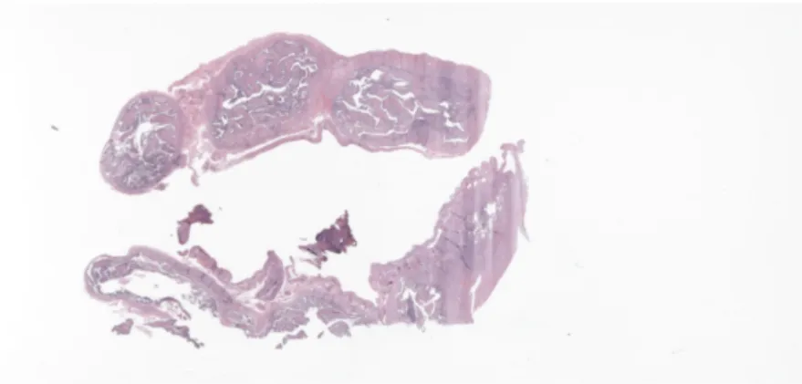
Medical image analysis is taking great advantages of the advances and latest break-throughs of image segmentation as it helps to optimize different kinds of measure-ments and reduce inaccuracies. Whole slide images (WSI) for example, are digitized conventional glass slides that are used by medical experts worldwide for different applications, such as diagnosis, research or education. There are several applications of image segmentation handling such digitized images. Figure 1.1 shows an example of a typical WSI.

WSIs are produced by utilizing specialized hardware and software. The former refers to a scanner which digitizes glass slides and the latter is used to visualize and analyze the resulting digitized images known as digital slides [2]. Such digital slides are usually high resolution images which may take enormous memory space [3]. This introduces new challenges as scanner manufacturers try to provide devices capable of producing high resolution digital slides in a short span of time.

It is here then, when image segmentation plays a vital role to deal with the problems of storage and time optimization. As it turns out, pre-localizing the tissue from slides can save up to 40% of the time required for scanning and it effectively reduces memory space [3]. Pre-localization of the tissue requires extracting the regions of the

(11)

1. Introduction 3

Figure 1.1 Whole slide image

slide image which correspond to the tissue and separate them from the background. The outcome of pre-localization is what is also referred to as mask. A mask indicates the regions in the slide image that should be scanned and the ones that should be ignored in order to save time and memory space. Overlaying the mask on the slide image produces an image as shown in Figure 1.2.

Figure 1.2 Localization of tissue

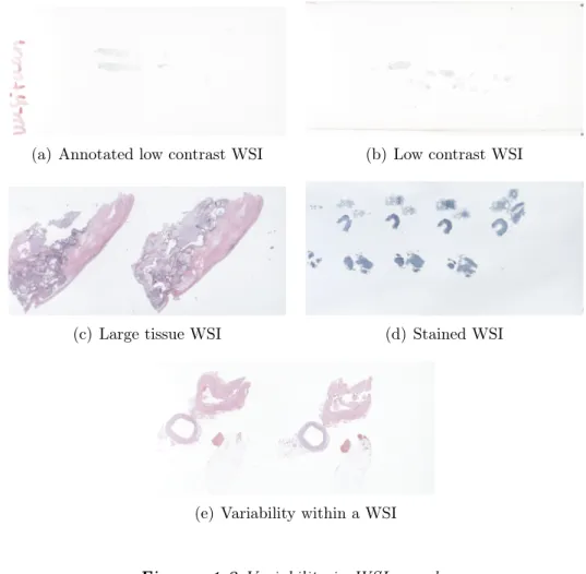
Despite of the numerous studies for pre-localizing tissue, it is not yet a trivial prob-lem. Physical glass slides are prone to contain artifacts such as dust particles, air bubbles and abnormalities which can make the segmentation process even more challenging. Moreover, the variability among samples should also be taken into ac-count. Samples usually vary depending on the size of the tissue, staining, color, shape and distribution [3]. Figure 1.3 shows an example of such variability, Figure 1.3(a) and Figure 1.3(b) for instance, present low contrast between the tissue and the background, opposite to Figure 1.3(c) which shows high contrast. There are also samples which have been stained as in the case of Figure1.3(d) where blue staining has been applied on the sample, that not only changes the background in compar-ison with other samples but also reduces the contrast between the tissue and the

(12)

1. Introduction 4

(a) Annotated low contrast WSI (b) Low contrast WSI

(c) Large tissue WSI (d) Stained WSI

(e) Variability within a WSI

Figure 1.3 Variability in WSI samples

background. Also samples such as the one in Figure 1.3(e) brings an extra challenge as the variability is present within the sample, there are sections of the tissue with high contrast but there are also some slices of tissue with low contrast. All in all, there are samples from which extracting the tissue can be a tough task, even for expert pathologists.

In this thesis work we examined two different deep learning architectures, namely UNet and DeepLabV3+, and assessed their performance for a company case. The company’s name is Jilab Inc, it is a Finnish company located in Tampere which offers a wide range of pathology services for customers around the globe. Jilab is looking forward to implementing a supervised learning method that allows for image segmentation and tissue extraction from WSIs. In adition to that, a desktop application was developed to annotate histopathological images which ultimately provided the data we used to train our algorithms.

In the next section, background information about the problem of image segmenta-tion is presented, followed by Secsegmenta-tion 3 where the concept of artificial neural networks

(13)

1. Introduction 5

is discussed. The models used in this thesis work are described in sections 4 and 5. Thereafter the results are presented and discussed in Section 7. Finally, conclusions are presented in Section 8.

(14)

6

2. IMAGE SEGMENTATION

Image segmentation is a process through which objects and regions of interest are separated from a given image. Objects are often predefined classes which are further on detected and separated from the rest of the content within the image. For instance, an image segmentation task could be separating human faces from a set of images, “human face” defines the class and the process would return a set of coordinates, pixels in this case, within which the objects are located. There could be more than one class to be separated from a single image. For example one could use image segmentation to separate not only human faces but also cars, cats and dogs from the same image. For tasks of this kind, bounding boxes are often used to indicate the location of such objects i.e, human faces. However, bounding boxes are not the focus of this work as we are interested in segmenting accurate contours of objects.

There are two general approaches for identifying and extracting objects from an image, region based segmentation and edge based segmentation [4]. The former identifies all the pixels that belong to a certain object whereas the latter returns only those pixels which define the boundary of the object.

Different methods have been developed in the field of image segmentation throughout the time. There are those methods based on pattern recognition techniques which compute the physical properties of an image in order to identify objects within it. Such properties can be the colors, the intensity of the colors, the gradient and so on, which are then computed and those regions or pixels with similar properties are clustered together and thus identifying objects in the image. The success image segmentation based on pattern recognition methods depends highly in the definition of the group of properties through which objects will be identified. It is however a considerable challenge in those cases where there is a big variability from image to image.

There is a more recent approach, which has shown to be very effective in the problem of image segmentation. It is artificial neural networks (ANN) which are based on distributed nonlinear parallel processing [4]. ANNs have demonstrated to be a very

(15)

2. Image Segmentation 7

(a) Input image (b) Pixel wise segmentation (c) Bounding box segmentation

Figure 2.1 Image segmentation example, Source: [5]

powerful tool in image segmentation problems and it is a very active research area nowadays. The methods presented in this thesis are based on them for which this topic will be analyzed further in Section 3. An ANN is a basic mathematical model of the human brain. An ANN is composed at its root level by computational units called neurons which receive one or multiple inputs and produce an output. There is usually a large number of neurons in an ANN which are interconnected forming different architectures in order to fulfill the functionality of the network.

When dealing with image segmentation problems there are some major challenges which are to be taken into account, some of them could be a considerable concern depending on the case of study. In most cases however, it will be very likely to encounter issues related to noise and in some cases computational resources may come up short. Noise can appear as undesired objects in the image samples which may require some prepossessing steps in order to get rid of them or at least diminish their effect, but noise can also be outlier samples which are not representative but they can produce misleading results. In this work, we will deal with different kinds of artifacts such as air bubbles, dust particles, which are present in some of the samples which are often misclassifed and we aim to perform a good segmentation despite of them.

Image segmentation has shown to be effective in various applications ranging from hand text recognition, sign gestures recognition, face recognition, medical images processing, among others. It has reduced the dependency on manual procedures as human errors also decrease.a basic examples of how image segmentation works is depicted in Figure 2.1. Three different classes are defined: cow, grass and water and they are to be segmented or separated from a given input image, Figure 2.1(a) is the input image and Figure 2.1(c) is the output where each pixel in the original image is assigned one of the classes predefined and thus the objects are separated from the original image.

(16)

2. Image Segmentation 8

Image segmentation methods are expected to work ideally as good or even better than what is shown in Figure 2.1 and in most cases a large number of sample images is involved, for that reason the algorithms should allow for a considerable level of variability between samples.

(17)

9

3. ARTIFICIAL NEURAL NETWORKS

An ANN is a basic mathematical representation or model of the human brain. It attempts to reproduce one of the most powerful capabilities of the human brain which is learning. The human brain can learn how to do numerous kinds of tasks, such as recognizing faces, driving, painting, etc. Artificial neural networks can learn, or more specifically they can be trained in order to predict and classify with the same accuracy of that of a human brain or even better in some cases.

Computers are far better and faster than humans when solving complex calculations in a very short time, however they are not capable of learning, not at least before machine learning was first introduced. By introducing neural networks we enable computers to learn in a very similar way as we humans do and learn from previous experiences. For example, if a neural network is to classify 10 different types of animals, it is fed with several images, it attempts to classify them one by one and compensates its errors. By repeating this process over and over again, the error of the network can be minimized and consequently its accuracy is maximized.

In general, the more samples that are fed to the ANN, the more experience it will gain, the more accurate it will be. Depending on how complex the task is, an ANN may need a large number of samples in order to be trained which brings a downside when using neural networks since it is sometimes very difficult to gather and handle that many samples.

An ANN consists of a large number of computational units referred to as neurons, each one of which receives one or multiple input values and produces one output. Neurons are interconnected and the information flows through such connections across the entire network.

In this section ANNs will be explained more in depth, taking into account the main components that conform an ANN and how it is trained. We will also review some architectures and topologies of artificial networks in Section 3.3.

(18)

3.1. Artificial Neuron 10

3.1 Artificial Neuron

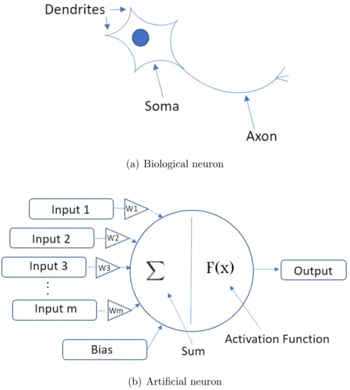
Biological neurons are composed of dendrites, one soma and an axon. Dendrites receive the information which is later processed within the soma and then the infor-mation is passed on to the axon which is connected to other neurons [6]. Analogically an artificial neuron receives the information in the form of inputs which are then weighted and summed together by arithmetic addition and then passes the result to a transfer function also referred to as activation function [7]. Figure 3.1 shows the representation of a biological (Fig 3.1(a)) and an artificial neuron (Fig 3.1(b)).

(a) Biological neuron

(b) Artificial neuron

Figure 3.1 Biological and artificial neuron

Mathematically speaking, each neuron ultimately represents a function that depends on the linear combination of the inputs as shown in eq. 3.1 where wis the weights, x is the inputs, b is bias, F is the activation function and the neuron output y is given by

(19)

3.2. Types of Activation Functions 11 y=F(wTx+b) (3.1) where x=hx1 x2 ... xn i , (3.2) w=hw1 w2 ... wn i . (3.3)

The ultimate goal is then finding those values ofwandb for each one of the neurons in the network, in such way that the network is capable of classifying and predicting accurately. The process through which those values are found is called learning and it is by learning that an ANN can gain experience. The weights in a neural network are "learned" as the network is trained and fed with more samples. This is explained in further in Section 3.4.

3.2 Types of Activation Functions

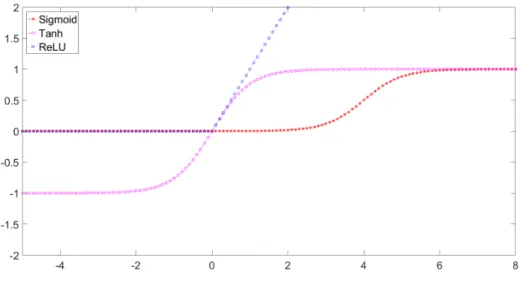
Activation functions allow for a nonlinear behaviour of an ANN and thus it is possi-ble to mimic the type of responses of a human brain. The most common activation functions used in ANNs are nonlinear Sigmoid and ReLU [8]. Using such activation functions allow the response of a neural network, approximate non-linear functions. However, there is a downside on using this kind of function as they can be com-putationally expensive [9] in contrast with linear functions. Choosing the type of activation functions to be used in the network depends heavily on the specific needs of each case. Activation functions limit the output range of each neuron [10] and ultimately the output range of the network itself.

• Sigmoid

The sigmoid function is not very computationally expensive when used in neural networks trained by backpropagation [10] and it is easily differentiable [11]. Training a neural network will be explained later in this section. The output range of the sigmoid function is (0,1) for any given real value. The characteristic curve is shown in Figure 3.2. The sigmoid function is also called logistic function and it is defined as in eq. 3.4 [12].

(20)

3.2. Types of Activation Functions 12

sgm(s) = 1

1 +e−s. (3.4)

• Hyperbolic Tangent Function

The hyperbolic tangent function is also a nonlinear function and ANNs using this function or functions of the same kind, exhibit nonlinear behaviour when there are enough neurons [13]. This function is one of the most commonly used among nonlinear activation functions [14].

The hyperbolic tangent function, as claimed by M. Bharathi and M. M. Rekha [15], presents a faster response compared to the sigmoid activation function, therefore it is of special interest when the application requires such behaviour. The output range of this function is (−1,1)for any real valuexand it is math-ematically defined as the ratio between the hyperbolic sine and the hyperbolic cosine functions (eq. 3.5) which equates the ratio of the half-difference and half-sum of two exponential functions [10]:

tanh(x) = sinh(x)

cosh(x) =

ex₋_e−x

ex₊_e−x. (3.5)

The characteristic curve of the hyperbolic tangent function is as shown in Figure 3.2.

• Rectified Linear Unit (ReLU)

The rectified linear unit is an unbounded activation function which has become very popular in deep learning [16]. It is of special interest due to its numerical properties [17]. As it is demonstrated by X. Glorot et al. [18], using the rectified linear unit as activation function makes a better representation of the biological neuron and it can produce better results than the hyperbolic tangent function. It is also referred to as hinge activation defined as:

g(u) = max(0, u). (3.6)

It simply returns 0 when u < 0 and returns linear function with slope equals to 1 otherwise as shown in Figure 3.2

Using the ReLU activation function is very advantageous when dealing with the vanishing gradient problem. The vanishing gradient problem is a well known issue in the context of deep neural networks and it occurs when the gradient of the loss function approaches zero as it decreases at every layer during backpropagation in such way that the layers closer to the input do not

(21)

3.3. Architecture of an Artificial Neural Network 13

Figure 3.2 Characteristic curves of activation functions

learn at all. This is explained in more detail in Section 3.4.2. In the case of the rectified linear function the result is always either 0when the input is less than 0 or 1 otherwise, and that is how the problem of vanishing problem is avoided [19].

3.3 Architecture of an Artificial Neural Network

An ANN consists of three main layers: input layer, hidden layers and output layer (Fig. 3.3).

• Input Layer: This layer receives the inputs. Such inputs are numerical values representing different types of data such as images, sound tracks and other kinds of signals.

• Hidden Layers: These layers connect the input layer to the output layer. They are responsible for extracting patterns [20]. Hidden layers are connected after one another which means that each layer will extract features based on the previous layer. There can be several hidden layers depending on the applica-tion.

• Output Layer: The output layer produces human readable result in contrast with the hidden layers where the output is often not straightforwardly under-standable. The output layer is connected to the previous hidden layers and it returns the final prediction and/or classification.

(22)

Figure 3.3 General Architecture of an ANN, Source: [20]

Figure 3.3 depicts an ANN composed by 2 hidden layers, but there can be many of them. Neural networks with multiple hidden layers are usually known as deep neural networks. Deep learning takes advantage of the powerful computational capabilities developed in the last couple of decades in order to process neural networks with several hidden layers.

The figure also shows that all the neurons from each layer are connected to each and everyone of the neurons of the next layer, however that is not always the case and there are scenarios where the layers are not fully connected. Using non-fully con-nected, also referred to as sparsely-connected neural networks, can bring advantages including improvement in accuracy performance as well as a decrease of the hard-ware energy consumption, which is usually a consequence of the high complexity of fully connected networks [21].

A. Ardakani et al.[21] proposed an architecture based on a sparsely-connected neural network and achieved results that show up to84%reduction in energy consumption and up to90% less in memory usage compared to fully connected neural networks. Networks where the information flows in one direction, are known as feedforward networks. Feedforward networks can be of the type multilayer perceptron (MLP), like the one shown in Figure 3.3, or they can be bridged multilayer perceptron (BMLP) [22]. BMLP topology allows connection across layers (Fig. 3.4), in contrast with MLP networks where layers are connected one after another. As a special case of BMLP there are fully connected cascade networks FCCN (Fig.3.4(b)) where each

(23)

one of the layers consists of one neuron only [23].

(a) Bridged Multilayer Perceptron (b) Fully Connected Cascade Networks

Figure 3.4 BMLP and FCCN, Source: [23]

One of the disadvantages when using MLP topologies is the uncertainty on how many hidden layers should be used. Using to many of them will make the network learn patterns that may be irrelevant for the task, on the other hand not using enough hidden layers will cause the network to be inaccurate [24]. In FCCN architectures however, the hidden layers are added one at a time as the network learns [25], which solves the problem brought up by using MLP architectures. Each one of the layers in a FCCN is composed of one neuron, and each neuron is connected to the original inputs and to the layers previously added. They are also connected to a bias input. There are other networks where information flows in two directions, they are bidi-rectional networks. In bidibidi-rectional networks it is possible for instance, to connect the output layer with their inputs. Such network is referred to as recurrent neural network (RNN) [26]. RNNs depend not only on the original input but also on the network’s previous results. RNNs are widely used for example, in adaptive filtering where given a stationary random process the network is capable of predicting fu-ture values [27]. Some other applications where RNNs have been used are motion detection, music synthesis and financial forecasting [28]

The possibility of connecting neurons and layers in various ways allow for different architecture types. Certain features and patterns can be detected easier using a type of architecture that suits best. For instance, there are architectures which can be very effective for recognizing sound patterns, while some other architectures are more suitable when addressing problems related to image segmentation.

(24)

3.4. Learning Process 16

3.4 Learning Process

The learning process is that through which an ANN gains experience. It allows the network to self-adjust its parameters, also called weights, to compensate its output error. In order to do so, there are three general steps performed during the learning process. First the network is presented pairs of input and output samples, input samples are those connected to the input layer of the network, and the output samples represent the desired output for those specific input samples. Second, the network processes the input samples throughout its layers and computes the error. Third, the network adjusts its parameters taking into account the last error obtained. Those three steps are iterated over and over until the error is minimized and converges if possible [29].

There are two major learning methods: supervised learning and unsupervised learn-ing. Supervised learning comprises those algorithms in which the desired output for a given set of input samples is known beforehand. The algorithm receives training samples and their corresponding correct classification referred to as ground truth. For instance, if the task of a network is to classify single handwritten letters, the learning algorithm receives images (with handwritten letters) as input and it also receives their corresponding classes eg. "a" , "b", "z"... The algorithm then passes the training samples through the layers of the network, compares the result at the output layer with the ground truth and computes the error. Supervised learning is also known as "Learning with a Teacher" [30] which brings up a clear analogy of having a teacher who knows the correct answers and corrects the student until it learns how to complete the task successfully.

In unsupervised learning in contrast, there is no teacher, in fact it is also referred to as "Learning without a teacher". There is lack of ground truth and the data is unlabeled. The task of a neural network based on unsupervised learning is finding a hidden and previously unknown structure in the data [31]. Unsupervised learning is a powerful tool in cases when labeled data is not available in large data sets and consequently it would take a long time to annotate or label all the samples. Some of the applications of unsupervised learning and neural networks are in the areas of computer vision, natural language processing, speech recognition, optimal control and networking [32].

The methods used in this thesis work are based on supervised learning methods. As it was mentioned previously, when training supervised learning based networks, one must provide the input samples and the ground truth which is the desired output for each one of the input samples. Training data as defined by J. Larsen [33] is:

(25)

T ={x(k), y(k)}Ntrain

k=1 , (3.7)

wherek is thek−thtraining sample, x(k)represents the input samples, y(k)is the desired output (ground truth) and Ntrain is the number of training samples.

3.4.1 Calculating the Error and the Loss

Once the input samples are passed through the neural network all the way to the output layer one can obtain the network’s output, let us name it yˆ(k). The error then is computed by calculating the difference between the ground truth y(k) and

ˆ

y(k), for values ofkranging from1toNtrain. The loss can be calculated by definition

with any mathematical function which returns a value that is proportional to the difference between y(k) and yˆ(k). It is also called cost function. One of the most common loss functions is the Mean Square Error (MSE) defined as:

E(w) = 1 Ntrain Ntrain X k=1 (y(k)−yˆ(k))2 = 1 Ntrain Ntrain X k=1 (y(k)−f(x(k),w))2, (3.8)

wherewrepresents the weights of the ANN and yˆ(k) is a function that depends on the input samplesx(k) and the weights was in eq. 3.9

ˆ

y(k) = f(x(k),w). (3.9)

However, there are other loss functions that have shown to be equally useful and even more efficient for certain tasks. G. Nasr et al. [34] for example, used ANNs to forecast the demand of gasoline from Lebanon during a seven year period between January 1993 to December 1999. During the training of network they used the cross entropy loss function (eq. 3.10) which proved to be faster and it also improved the overall performance of the network compared to the MSE loss function.

(26)

3.4. Learning Process 18 E(w) = 1 Ntrain Ntrain X k=1 [ˆy(k) lny(k) + (1−yˆ(k)) ln (1−y(k))] = 1 Ntrain Ntrain X k=1 [f(x(k),w) lny(k) + (1−f(x(k),w) ln (1−y(k))]. (3.10)

The aim is to minimize the loss function such that it reaches the minimum value possible. The loss function is continuous and differentiable with respect to the weights w. In other words, one must find those optimum values of w such that E(w) is minimized and the accuracy of the network is maximized. The loss E(w)

can contain many local minima and there are no practical methods that guarantee a global minimum [33]. The gradient of the loss function with respect to the weights wreturns the variation of E(w)with respect tow. Therefore when the values ofw are optimal the value of the gradient of the loss function approaches zero. Letwˆ be the optimal values ofw, then:

∇E( ˆw) = ∂E(w) ∂w w= ˆw = " ∂E(w) ∂w1 w= ˆw , ..., ∂E(w) ∂wm w= ˆw #T = 0, (3.11)

wherem is the number of weights.

3.4.2 Backpropagation

Backpropagation uses the gradient descend in the learning algorithm [35]. ANNs learn through an iterative process in which the error is computed on every training sample and the weights are updated accordingly. Initially the weights ware initial-ized with zeroes or pre-initialinitial-ized values other than zero. In general the weights are updated in accordance with the direction where the loss function has the steepest descend. This method known as steepest descend was proposed by Cauchy in 1847 [36] and it shows that the update of wis as follows:

wj+1 =wj −η∇E(wj), (3.12)

wherewj corresponds to the values of the previous iteration, η is the step size and

(27)

If given a proper step size η, the loss should decrease such that:

E(wj+1)< E(wj). (3.13)

While eq. 3.12 guarantees an update towards the direction of the steepest descend it does not necesarly guarantee eq. 3.13 as it depends on the value of step size η. It turns out choosing a proper value of η is pivotal and it is not trivial. A value of η that is too small means that it will take too many iterations for the algorithm to minimize E(w), and a value of η that is too large will prevent the algorithm from converging as shown in Figure 3.5 where the loss function is a quadratic function with two weights and its result is plotted on every iteration step. In Figure 3.5(a) for instance, the step size is too small and the loss function converges but it takes many steps to find the valley of the function. Whereas in Figure 3.5(b) the step size is too large and therefore the loss function diverges.

(a) Small Step Size (b) Large Step Size

Figure 3.5 Step Size, Source: [33]

Overcoming this challenge leads to a solution in which the step-size is not fixed as in eq. 3.12, instead, it adjusts the step-size as it iterates (eq. 3.14), that is an adaptive step size. That way, it is reasonable to start with a rather large step-size and then make it smaller as the algorithm approximates a minimum.

(28)

The difference between a fixed step size and an adaptive step size is shown in Figure 3.6. Using an adaptive step size optimizes the number of iterations to make the loss function converge faster (Fig.3.6(b)) as compared with a fixed step size where it takes many more iterations to minimize the loss function (Fig.3.6(a)).

(a) Fixed Step Size (b) Adaptive Step Size

Figure 3.6 Fixed Step Size vs. Adaptive Step Size, Source: [33]

Different methods to find an optimal value of ηj have been proposed such as the

Cauchy step-size or BB step-size. Dai and Yuan also proposed an alternate mini-mization gradient method which improves Cauchy’s slow converge [36]. It is achieved by minimizing not only the loss function but also the norm of the gradient alter-nately.

Since the steepest descend is an approximation method, one should decide when to stop iterating. There are different criteria in which one could base on in order to stop iterating. One simple criterion is for example to stop if the change in the loss function from one iteration to another is small enough [33]. This criterion is:

|E(wj)−E(wj+1)|< τcost. (3.15)

Eq. 3.15 however, does not guarantee that the algorithm is close to a minimum which is determined by 3.11. There is another criterion which deals with that issue [33], it is:

(29)

This criterion is based not on the loss function as in eq. 3.15 but on its gradi-ent. According to eq. 3.16 the iteration should stop when the euclidean length (|| ∇E(wj)||2) is smaller than τgrad which is a small constant.

From eq. 3.9 we see that the output of a neural network can be represented as function whose parameters are the input samples and the weights. A general repre-sentation of the system of a network such as the one in Figure. 3.3 is:

Figure 3.7 ANN - Black Box

wheref(x,w)is composed by as many layers there are, so it can be split as follows:

Figure 3.8 ANN Composition

where h1 represents the first layer, h2 represents the second layer, so on and so

forth until the i−th layer. Since f(x,w) is really a composed function it can be rather difficult to calculate the gradient of the loss function (eq. 3.8) based on it. However, as it was demonstrated by J. Larsen [33], the gradient of the loss function can be calculated efficiently using backpropagation of errors.

Backpropagation calculates the error at the last layer and then propagates it back to the previous layer in order to update the weights w. This method calculates the gradient of the loss function with respect to the weights of each one of the layers and update them accordingly. It can be shown for an ANN that ifwij is the weight

connecting the output of the neuron j from the layer l-1, and the neuron i from the layerl then:

(30)

3.4. Learning Process 22 ∂E(w) ∂wij =− 1 Ntrain Ntrain X k=1 δixj, (3.17)

where δi is the error calculated for the neuron i to which the weight is connected,

andxj is the result of the linear activation of the neuron j from which the weight is

connected [33]. This way, while the error produced at the hidden layers is unknown, the error at the last layer can be easily computed in terms of the network output errory(k)−yˆ(k)and the derivative of its activation function as follows:

δi(k) = (y(k)−yˆ(k))ψi0(ui(k)), (3.18)

whereψi(ui(k))is the activation function of the neuroni, andψ0i(ui(k))is its

deriva-tive. Then,ui(k) is defined as:

ui(k) = nH

X

j=1

wijhj(k) +wi0, (3.19)

where nH is the number of connections from the previous layer, and hj(k) is the

output of thej−th neuron from the previous layer The error for the hidden layers is computed as follows:

δj(k) =δi(k)wijψj0(uj(k)). (3.20)

From there on, it is possible to calculate the error at previous layers straightforwardly following eq. 3.17. The backpropagation algorithm using the gradient descend consists of the following steps:

1. Initialize weights w.

2. Pass every training sample through the network and calculate yˆ(k) for each, and the output for each layer.

(31)

3.5. Convolutional Neural Networks 23

3. Compute the errors as error(k) = y(k)−yˆ(k).

4. Compute the gradients of the loss function using backpropagation (eq. 3.17). 5. Update the weights for each layer using eq. 3.12.

6. Iterate from step 2 until the stopping criteria (eq. 3.16) is fulfilled.

On a neural network with multiple layers however, there appears a problem when using backpropagation. As the error propagates backwards, the gradients with re-spect to the weights (eq. 3.17) tend to be smaller and smaller and approach zero. Since the update of the weights is proportional to the value of the gradient, the layers at the beginning of the network (closer to the input layer) will learn slower in comparison with the layers placed at the end which learn a lot faster. This is known as thevanishing gradient problem.

The vanishing gradient problem happens as a consequence of the derivative terms which are usually less than 1. As it is propagated with successive multiplications, the gradient tends to zero. Also, if the gradient of the activation function returns values larger than 1 then it will cause the opposite effect and the gradient will diverge [37]. Therefore, instead of using traditional activation functions such assigmoid ortanh previously studied in Section 3.2, using ReLU as activation function mitigates with the problem of the vanishing gradient and it is less computationally expensive to compute [38]. It is explained by the nature of the ReLU function, as its gradient is always 1 for values larger than zero and zero otherwise. There are other activation functions which also alleviate the problem of the vanishing gradient such as the exponential linear unit (ELU), the parametric exponential linear unit (PELU) or the scaled exponential linear unit (SELU) [37].

3.5 Convolutional Neural Networks

A convolutional neural network is a specific type of ANN. They are a very powerful tool when it comes to image classification and object recognition tasks. In fact, CNNs have demonstrated to be so effective that sometimes they have outperformed humans in various tasks [39]. C. Szegedy et al. [40] pushed the state of the art for classification and detection when they put together a CNN architecture named "Inception" with which they achieved outstanding results using much less parame-ters in the network, therefore less consumption of computational resources and yet improving the accuracy.

(32)

Aiming at reducing the number of parameters in a CNN is of special interest as it deals with one of the most common limitations of CNNs which is the high demand of computational resources. Convolutional neural networks have proved to be effective for image classification tasks and machine learning problems [41], however computa-tional resources may come up short when dealing with high resolution images, which have made the use GPUs very popular in this field. GPUs paired with optimized implementations of 2D convolutions facilitates the training of deep (several hidden layers) CNNs [42]. Despite of the advantages of using GPUs, this issue is far from being resolved and convolutional networks are often limited by the amount of mem-ory available as well as the speed at which GPUs can operate, consequently causing a long time required for training and classification [42].

CNNs are used to extract patterns and classify images, or image-like data. They also consist of neurons which self-adjust during the learning phase, and just like in an ANN, neurons receive an input, they perform an operation over the input and pass the result to an activation function [43]. However, in comparison with a traditional ANN, a CNN uses spatial information between the pixels of an image by using discrete convolution [44]. Each layer of a CNN will produce an array of feature maps, which are specific features extracted at all locations of the input [45]. For instance, a feature map may represent the sharp edges of an image, another feature map may indicate locations with high contrasts, so on and so forth. Feature maps produced by one layer are then passed on to the next layer which will produce another set of feature maps based on the input.

3.5.1 Discrete convolution

CNNs extract features from images by using discrete convolution between the input and different kernels. In Figure 3.9 for example, two different features were extracted from Figure 3.9(a). The first feature is the result of the convolution between the original image and a kernel which highlights the horizontal edges of the picture (Fig. 3.9(b)). Likewise, a second kernel highlights the vertical edges from the input image when it is convolution-ed with the original picture (Fig. 3.9(c)).

In a convolutional neural network, the first layers (the ones closer to the input layer) usually extract basic patterns and features such as the ones in Figure 3.9. However, further layers extract much more complicated features from the images. As a matter of fact, when going through the results of each one of the layers, the features extracted by a deep convolutional neural network (DCNN) may become not at all unidentifiable by humans, in other words, it may be very hard to explain

(33)

why certain network classifies a certain image the way it does just by looking at the features extracted across its layers.

Using a proper number of layers is also very relevant. If the network is too large, it may be extracting features which are actually not relevant for the task, but if there are not enough layers, the network may be missing some features which can be important for the task as those missing features could improve the performance of the network.

(a) Original Image (b) Horizontal edges (c) Vertical edges

Figure 3.9 Feature extraction, Source: [46]

To better understand discrete convolution, let us explain first the mathematical definition. Let f be a function of two variables f(x, y) and g be a function of two variablesg(x, y). Then the convolution of f and g is f ∗g:

(f ∗g)(x, y) = +∞ X u=−∞ +∞ X v=−∞ f(u, v)g(x−u, y−v). (3.21)

We can extrapolate from here to define the convolution of matrices since they can also be expressed as a function of x and y as: Axy = f(x, y), where A is a matrix

of dimensions n×m and Bxy = g(x, y), where B is a matrix of size k ×l. The

convolution f∗g then produces a matrix C of size (n+k)×(m+l):

cxy = X u X v auvbx−u,y−v, (3.22)

(34)

white image andB is a convolutional kernel, then eq. 3.22 is a typical convolutional operation in a CNN.

According to eq. 3.22 the kernel B is flipped in both axis due to the negative subscripts −u and −v. However, flipping the kernels is computationally expensive since it takes longer to feedforward the CNN and backpropagate the error [48]. For that reason, it is usually preferred to use cross-correlation instead of convolution. Cross-correlation is almost the same as convolution except that it does not flip the kernels, therefore same results can be achieved in considerably less time. Cross-correlation is defined as follows:

cxy = X u X v auvbx+u,y+v. (3.23)

Note how b subscripts u and v are no longer negative, which indicates there is no need to flip over the kernel B.

Convolution and cross-correlation operations can be thought of as a sliding window (the kernel) which maps the values of the image and forms a new one, in which certain features are extracted as in Figure 3.10. Let us suppose that our kernel B is a 3×3 matrix and our image is the matrix A of the same size, like this:

A=    2 3 1 0 5 1 1 0 8    B =    0 −1 0 −1 5 −1 0 −1 0   . (3.24)

We have chosen B to be symmetric for the sake of simplicity just so eq. 3.22 and eq. 3.23 both hold.

The result of A∗B in this case equals the result of the cross-correlation RAB as

follows: RAB =A∗B =    2 3 1 0 5 1 1 0 8   ∗    0 −1 0 −1 5 −1 0 −1 0   =    7 7 1 −8 21 −9 5 −14 39   . (3.25)

(35)

(a) First iteration (b) Second iteration

(c) Third iteration

Figure 3.10 Convolution and Cross-correlation, Source: [49]

The values contained in matrixB are in fact some of the weights wof a more extend CNN. Those values are self-adjusted during the learning process. The number and size of the kernels will define the number of parameters to train in the network. If a CNN is composed by j number of kernels, and all kernels are of the same size k×l, then the number of parameters which need to be trained is j×k×l. This holds for 2D images, but if the images are RGB valued, the number of parameters is three times larger.

From eq. 3.21 we can see that the kernel acts as a 2-D sliding window which maps the input sample, we can also see that it slides from−∞to+∞ in both axis. However, in this case images are only defined within the range of their size and for this reason convolution from−∞to+∞is not possible unless the image is padded with zeroes in both axis, only then such convolution would be possible. Furthermore, convolutions with an infinite range are of course not possible using a computer which can only iterate a finite number of times. Convolutions has to be limited to a reasonable range so it can be computed. There are different alternatives: a) set the limits of the convolution such that the kernel only maps those values which are previously defined, b) set the limits of the convolution in such way that the result keeps the resolution and dimensions of the original input. In that case the input sample may have to be padded with zeroes. Or c), set the limits of the convolution such that the result is a map of higher resolution, for which it would be necessary to pad the input image with zeroes.

There are three basic parameters which defined a convolution operation: the kernel size, the stride and the padding. The kernel size simply defines the dimensions of the convolutional kernel. The stride is the step size the kernel will move across the

(36)

input sample. That is the amount of pixels the kernel is translated horizontally and then vertically as it is convolution-ed [50]. Figure 3.11 illustrates a convolution operation between an input sample of size 5×5 and a kernel of size 3×3 with a stride set to 2. A convolution with no stride, or stride set to 1 follows the basic definition of convolution as shown in Figure 3.10. And finally the padding is the amount of rows and columns of zero values added around the input sample.

Figure 3.11 Convolution with stride set to 2, Source: [50]

As the image is passed through the layers, the convolutional kernels reduce the size of the input sample, therefore some resolution is lost after every convolution. This can become a problem specially with networks composed by many convolutional layers [50].

Let us take a look at the different types of convolutions there are. Besides normal convolution, as the ones explained so far, there is also dilated convolutions and transposed convolutions.

• Dilated convolutions: Dilated convolutions can be thought of as "dilated" kernels. That means adding zeroes between the elements of the kernel. That will increase the field of view of the kernel without increasing the parameters. In dilated convolutions a kernel of size k×k turns into a kernel of k+ (k−

1)(r−1) where r is the dilated stride, thus it allows the extraction of multi-scale contextual information while keeping the resolution [51]. That means that every pixel at the output of the convolution is the result of mapping more pixels from the original input sample while keeping the number of parameters. Different convolutions with dilated kernels are shown in Figure 3.12. The squares in yellow belong to the elements of the kernel and the background squares in blue represent the input sample. While Figure 3.12(a) shows a kernel with no dilation, kernels in Figure 3.12(b) and Figure 3.12(c) have a dilation rate of 2 and 3 respectively. A 2-D dilated convolution is defined as in eq. 3.26.

(37)

(a) No dilation (b) Dilation rate 2 (c) Dilation rate 3

Figure 3.12 Dilated Convolutions, Source: [51]

cxy = X u X v auvbx+u×r,y+v×r (3.26)

• Transposed convolutions: Transposed convolutions generate feature maps with higher resolution out of the input sample. That is, for every pixel in the input sample, multiple pixels are produced at the output as a result of the transposed convolution. In other words it up-samples the input sample. It takes as parameters a dilation rate for the input feature map and the padding which is the number of columns and rows to be added around the input sample. Transposed convolutions are often referred to as inverse convolution or de-convolutions due to the fact that it is possible to recover the spatial resolution lost after performing a regular convolution. However transposed convolution is not the inverse function of convolution in the strict mathematical sense. In fact it does nothing different that normal convolution operations, except for the padding and dilation rate applied to the input feature sample.

Transposed convolutions are very useful in tasks related to localization, seman-tic segmentation, super resolution, visualization, visual question answering and recognition [52]. L. Xu et al. [53] presented how transponsed convolutions can be used to deal with artifacts caused by convolution operations. They devised a solution where a separable structure is introduced for deconvolution against artifacts.

Figure 3.13 shows how transposed convolution is performed, the squares in blue represent the original pixels from the input feature map, the input sam-ple is dilated ×2 and then zero padded. The squares in green represent the output of the transposed convolution. In this case a feature map with spatial resolution of 5×5was obtained out of an input sample with spatial resolution

(38)

of 2×2 using a3×3 convolutional kernel.

(a) (b) (c)

Figure 3.13 Transposed Convolutions, Source: [54]

3.5.2 Layers of a Convolutional Neural Network

There are various types of CNN architectures, however there are three types of layers which are used in most architectures: convolutional layers, pooling layers and fully-connected layers [52], (see Figure 3.14).

• Convolutional layers: These layers use convolution kernels in order to ex-tract the features from the input image or feature maps as previously explained in Section 3.5.1. There may be several convolution kernels per layer depending on how many features are intended to be obtained in each. Convolutional lay-ers also perform transposed convolutions, often referred to as de-convolutions or inverse convolutions. Feature maps produced by one layer are usually passed on to a pooling layer, or directly to the next convolutional layer in case there is no intermediate layer. That is why convolutional layers accept as input either the original image or the feature maps produced from the previous layer. In order to introduce the capability of the network to learn non-linear features, each one of the values in every feature map, is passed to an activation function like the ones mentioned in Section 3.2. ReLU is a rather common activation function in this context as it has shown to improve the discriminative perfor-mance [55]. Tanh is also a common alternative as activation function in CNNs [52].

(39)

• Pooling layers: The intermediate layers are usually pooling layers. They do not add extra parameters to the CNN since they only perform fixed transfor-mations to the feature maps. Pooling layers reduce the spatial resolution of the input feature map and by doing so they achieve shift-invariance [52], that means that the network is more resilient towards displacements of the input images, which is in most cases a desirable behaviour in a CNN. Pooling layers also make convolutional neural networks more robust to distortions and noise commonly present in the input samples [56].

Pooling operations replace groups of pixels in the input feature maps by a representative value. Such representative value is usually the maximum value among the group of pixels or the average value. These operations are known as max-pooling and average pooling respectively. Max pooling has proved to make the CNN converge faster as it filters in stronger invariant features and therefore the CNN is capable of dealing with disturbances more accurately as the generalization performance improves [57].

In the context of CNN, pooling size is usually (2,2), where each of these numbers are the factors by which the input map is down-scaled in the vertical dimension and the horizontal dimension. Thus, if the pooling size is (2,2)the original spatial resolution is reduced by half in each dimension.

J. Nagi et al. [57] achieved an important improvement in the task of hand gestures recognition by putting together a CNN and max-pooling operations (MPCNN) achieving an accuracy of 96% where the task was classifying six dif-ferent gestures. H. Wu and X. Gu [58] demonstrated the utility of combining pooling layers with dropout operations, referred to as max-pooling dropout. In contrast with a fully-connected networks, non-fully-connected networks imple-menting dropout randomly disconnect nodes during the training phase which prevents the network from over-fitting.

Over-fitting is a well known problem in the context of neural networks. It happens when a neural network learns how to classify correctly the training samples and in some cases it may even have an accuracy very close to 100% over the training samples, but then accuracy plummets when the model is tested with samples previously unseen by the network [59]. In that scenario the model is over-fitted to the training data. Using dropout in CNNs on supervised learning has shown to improve the performance in various tasks such as speech recognition, document classification and vision [60].

According to H. Wu and X. Gu [58], using dropout before max-pooling layers can improve the performance of a CNN as it introduces stochasticity. Max-pooling layers select the highest value from a specific region in the input feature

(40)

map, causing that other units in the region are not taken into account at all for further processing. Average-pooling on the other hand, takes all the units into consideration by computing the average between them in a specific region of the input map, thus high activation units may be outshone by many other low activations [58]. That is why stochasticity introduced by max-pooling dropout plays a vital role in improving the CNN performance.

• Fully-connected layers: These layers are in charge of making high level abstractions. They are often used as the output layer of the CNN. Each one of the neurons in a fully-connected layer receives connections from all of the activation units from the previous layer, whether it is convolutional layer or a pooling layer. Let us suppose that a given model classifies hand written single digit numbers within the classes0to9, where the last layer is a fully-connected layer and the previous layer outputs a set of feature maps. The last layer would then consist of ten neurons, each one of which receives connections from all the activation units coming from all of the feature maps of the preceding layer. The last layer’s output is then an array of probabilities where each element describes the likeliness of the input sample of belonging to one of the classes. In some other architectures, fully connected layers are not used as the output layer, they are used instead as feature extraction layers placed before the output layers. Setting up and selecting the layers is tightly related to the classification task of the CNN. In some cases it can be even more accurate not to use fully connected layers for extracting high level features, and instead use features extracted from previous layers to train Random Forest or SVM algorithms [61].

All in all, a general representation of a convolutional neural network is shown in Figure 3.14 where the basic elements mentioned above are put together. The input layer receives the input images, from there on a series of hidden layers are concatenated one after another. The hidden layers compute convolutional operations with kernels and non-linear activation functions in order to produce a stack of feature maps which are then passed through a pooling operation. In Figure 3.14 max-pooling as max-pooling operation is used, however it can be average-max-pooling, max-max-pooling dropout or similar. Then the final feature maps are vectorized and fed to a fully connected layer which finally makes the classification. Depending on the task, the classification can be set to be binary or multi-class classification.

(41)

Figure 3.14 CNN - Basic Architecture, Source: [62]

3.5.3 Popular Architectures

As convolutional neural networks continue to push the boundaries in machine learn-ing, some particular architectures have become very popular across solutions and they are often used as a baseline for new architectures. Some of the most known architectures in the context of CNN will be described in this section.

• LeNet-5: Y. Lecun et al. [63] compared various methods in the task of hand-written character recognition. They observed that multilayer neural networks based on the Gradient-Based Learning technique showed better results com-pared to all other techniques specially if they are designed to deal with samples containing high variability. That is how they proposed a rather simple archi-tecture called LeNet-5 which was trained for digits recognition. It consists of seven layers not including the input (Fig. 3.15).

Figure 3.15 LeNet-5 Architecture, Source: [63]

The input is an image of size32×32and it is followed by a set of convolutional layers and subsampling layers. The first layer connected to the input, shown in the figure as C1, is a convolutional layer with 6 feature maps. The kernel

(42)

size used in the first layer is5×5. The size of the feature maps is28×28. The convolution is computed only for the valid regions of the input image. That means that the input image was not zero padded and therefore the spatial resolution of the feature maps is smaller by four pixels in each dimension. The total number of trainable parameters in the first layer is then (kernel size + bias input) × number of feature maps =(5×5 + 1)×6 = 156.

The subsequent layerS2 sub-samples the feature maps and reduces the spatial resolution by half. This operation is done by adding the activations of non-overlapping adjacent regions of size 4×4in the feature maps, then multiplied by a trainable parameter and added to a bias that is also trainable. The result is then passed to a sigmoidal activation function. The number of parameters added in this layer is 12.

LayerC3 is again a convolutional layer. It maps the feature maps fromS2 into 16 new feature maps. Every feature map in C3 is not however, connected to every feature map in S2. Therefore, the number of connections is reduced and it also causes that every feature map inC3 is learnt from different feature maps ofS2, thus breaking the symmetry in the network [63]. C3 adds 1516 trainable parameters. Layer S4 sub-samples the feature maps of C3 performing the same operations as in layer S2 adding 32 trainable parameters.

Layer C5 is a convolutional layer which operates with a kernel size of 5×5. Since the size of the feature maps produced by S4 is also 5×5, C5 outputs

1×1 feature maps. This layer adds 48120 more trainable parameters.

The next layer F6 is a fully-connected layer and it consists of 84 units as it was designed by Y. Lecun et al. [63] to represent a stylized image of the corresponding output class. It adds 10164 trainable parameters to the network. And finally the output layer predicts the class, it is fully-connected to F6 and it consists of one Euclidean Radial Basis Function (RBF) unit per class. • AlexNet: Researchers from the University of Toronto in 2012, trained a

con-volutional neural network to classify 1.2 million images into 1000 different classes [64]. It consists of five convolutional layers and three fully connected layers. One more layer at the end of the network makes the prediction into the different classes using softmax. Using softmax to make the prediction guaran-tees that all the values sum up to 1 so the output of the network represents a normalized probability distribution. AlexNet architecture is shown in Figure 3.16.

The total number of trainable parameters in AlexNet architecture is 60 mil-lion. This architecture was used for the ImageNet LSVRC-2010 competition

(43)

Figure 3.16 AlexNet Architecture, Source: [63]

obtaining the first place in the contest. Some of the novel features of the AlexNet are: a) Using ReLU as activation function in the hidden layers. Such feature makes the network learn faster than networks using saturated non-linear activation functions such as tanh. b) Training on multiple GPUs. Two GPUss were used to train the network putting half of the neurons in each. c) Local response normalization. AlexNet implements normalization after apply-ing ReLU for some of the layers. This feature reduced the error rate of the network in the ImageNet LSVRC-2010 competition. d) Overlapping pooling. Pooling layers do not usually overlap, but in this network using such kind of pooling avoids the network from overfitting and also reduced the network’s error rate compared to non-overlapping pooling layers.

• GoogleLeNet -"Inception": This architecture consists of a model in which optimal stages of the network are approximated by readily dense components [40]. This network contains repetitive modules stacked one after another, with max-pooling layers in some of the layers in order to reduce the spatial resolution by half. The module used at the core of this architecture is shown in Figure 3.17

where 1× 1 convolution modules in yellow are used to reduce the dimen-sion. This architecture optimizes the use of computational resources by using the dimensionality reduction characteristic aspect and consequently allows in-creasing the number of units while keeping the computational complexity from growing rapidly. Another important aspect of this network is the concatena-tion filters in which convoluconcatena-tions from multiple scales are combined together and that allows the network to process features at various scales simultane-ously. Inception achieved a big leap quality wise by using DCNNs with a subtle increase in the computational requirements as compared with smaller architectures.

(44)

Figure 3.17 Inception Module, Source: [40]

The nameInceptioncomes from the capability of this network to go deeper and deeper by simply adding pre-made blocks such as the one shown in Figure 3.17. Therefore, it allows to get higher level features straightforwardly. GooleLeNet (Fig. 3.18) is a special kind of an Inception architecture which consists of 22 layers. In order to deal with the vanishing gradient problem, authors of GoogleLeNet added auxiliary classifiers connected to the intermediate layers and added their loss to the the total loss of the network during training. The auxiliary networks are composed of an average pooling layer, followed by a

1×1 convolutional layer, a fully connected layer, a 70% ratio dropout layer and a classifier layer using softmax.

Figure 3.18 GoogleLeNet Network, Source: [40]

Figure 3.18 shows GoogleLeNet’s architecture where the blocks in blue are convolutional and fully-connected layers, blocks in red are pooling layers, blocks in green are depth concatenation layers, and blocks in yellow repre-sent softmax activations. The dotted line in the middle reprerepre-sents all the repetitive blocks as the one shown in Figure 3.17, which are stacked one after another.

(45)

It is very clear at this point, that the Inception architecture allows to extract deeper features very easily by simply designing one optimize convolutional block (Fig. 3.17) and using it over and over again depending on the desired depth of the network.

• Xception - "Extreme Inception": This architecture is a linear stack of depthwise separable convolution layers with residual connections [65]. It is based on an Inception module but taken to "extremes" as shown in Figure 3.19. The xception module is very similar to a depthwise separable convolu-tion. A depthwise separable convolution consists of two steps, the first is called separable convolution and it is simply a spatial convolution that is performed independently over each channel, therefore, it uses as many kernels as there are channels in the input. Note that so far the number of channels has not been incremented. This is followed by step two, which is a pointwise convolu-tion that will be used to increment the number of channels of the output. A pointwise convolution is based on spatial convolutions operated with kernels of size 1×1×k, where k is the number channels of the input. The number of such kernels corresponds to the number of channels desired at the output. All in all, depthwise separable convolutions are much less computationally expen-sive as compared to a regular spatial convolutions because the total number of multiplications computed during the convolutions is reduced.

(a) Inception module (b) Xception module

Figure 3.19 Comparison between the Inception module and the Xception module,

Source: [65]

The main differences between an Inception module and an Extreme module are the order of the operations and the non-linearities after the first operation. The former refers to the fact that depthwise separable convolutions perform channel-wise spatial convolutions first and they are then followed by 1× 1

convolutions, whereas in the Inception module1×1convolutions are performed first. The latter refers to the absence of ReLU non-linearity in depthwise separable convolutions as compared to the Inception module where ReLU non-linearity is performed after both operations, namely 1×1 convolutions and

(46)

spatial convolutions [65].

• VGGNet: This network was published by K. Simonyan and A. Zisserman [66] and it is aimed to classify large scale images. VGGNet is a convolutional neural network which extends the depth to 16 and 19 layers showing a significant improvement as compared to prior architectures.

VGGNet consists of a stack of convolutional layers which use 3×3filters with 1 pixel as convolutional stride and the spatial resolution is kept by padding the input of each convolutional layer. Some of those convolutional layers are followed by a 2×2 max-pooling layer with stride 2.

Then at the end of the network, there is a stack of three fully-connected layers, the last of those three performs a classification into 1000 different classes. All of the convolutional layers use ReLU as non-linear activation function. By slight variations of this general architecture, K. Simonyan and A. Zisserman [66] built different configurations of VGGNet which differ mainly in the depth, starting from 11 layers (8 convolutional layers and 3 fully-connected layers) and deeper configurations which use up to 19 layers (16 convolutional layers and 3 fully-connected layers).

Due to the depth of this network and the number of trainable parameters, it took from two to three weeks to train one model. It can of course be improved by using more powerful computer resources. For the ImageNet Large-Scale Visual Recognition Challenge (ILSVRC), the VGG network was trained us-ing an optimized version of the multinominal logistic regression implementus-ing mini-batch gradient descent with momentum and the weights were initialized by training a much shallower version of the network using only some of the first layers and the fully-connected layers at the end, and then keeping the weights obtained to initialize the network before training, thus reducing the training time.

Despite its simplicity, VGG network demonstrates how much better the results can be just by going deeper and adding more convolutional layers for large scale image classification. Figure 3.20 depicts the basic setup of VGGNet.

The main difference between VGGNet and other deep networks used for large scale image classification, is the use of convolutional filters with a rather small receptive field of 3×3 across the whole network. This network achieved the state of the art on the ILSVRC and also demonstrated to be very accurate for various image recognition data sets [66].

• ResNet: As computer resources become more powerful, neural networks have explored going deeper and deeper due to the benefits of deep neural networks