Data Migration in Heterogeneous Storage Systems
Chadi Kari
Department of Computer Science and Engineering
University of Connecticut Storrs, CT 06269 Email: [email protected]
Yoo-Ah Kim
Department of Computer Science and Engineering
University of Connecticut Storrs, CT 06269 Email: [email protected]
Alexander Russell Department of Computer Science
and Engineering University of Connecticut
Storrs, CT 06269 Email: [email protected]
Abstract—Large-scale storage systems are crucial components in data-intensive applications such as search engine clusters, video-on-demand servers, sensor networks and grid computing. A storage server typically consists of a set of storage devices. In such systems, data layouts may need to be reconfigured over time for load balancing or in the event of system failure/upgrades. It is critical to migrate data to their target locations as quickly as possible to obtain the best performance. Most of the previous results on data migration assume that each storage node can perform only one data transfer at a time. A storage node, how-ever, can typically handle multiple transfers simultaneously and this can reduce the total migration time significantly. Moreover, storage devices tend to have heterogeneous capabilities as devices may be added over time due to storage demand increase.
In this paper, we consider the heterogeneous data migration problem, where we assume that each storage nodevhas different transfer constraintcv, which represents how manysimultaneous transfersv can handle. We develop algorithms to minimize the data migration time. We show that it is possible to find an optimal migration schedule when allcvs are even. Furthermore, though the problem isNP-hard in general, we give an efficient algorithm that offers a rigorous(1 +o(1))-approximation guarantee.
I. INTRODUCTION
Large-scale storage systems are crucial components for today’s data-intensive applications such as search engine clusters, video-on-demand servers, sensor networks, and grid computing. A storage cluster can consist of several hundreds to thousands of storage devices, which are typically connected using a dedicated high-speed network. In such systems, data locations may have to be changed over time for load balancing or in the event of disk addition and removal. It is critical to mi-grate data to their target disks as quickly as possible to obtain the best performance of the system since the storage system will perform sub-optimally until migrations are finished.
For example, in a system consisting of parallel disks, data layouts are computed based on many factors such as user demands and disk space constraints to balance the load. Data layouts need to be changed over time according to changes of user demand patterns. In these cases, data need to be quickly moved to their target disks to obtain a new data layout as soon as possible.
Another example of data migration is when we add or remove disks in a storage system. In a large-scale storage system, disk removals, additions and replacements can occur frequently. For example, in a search engine cluster with
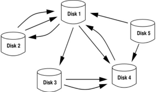
Fig. 1. An example of data transfer instance
hundreds of storage devices, such system upgrades and re-placements are required as often as every few days [1]. In the event of disk additions and removals, it is necessary to quickly redistribute or recover data so that the system can run in the best performance under the new configuration.
The data migration problem can be informally defined as follows. We have a set of disks v1, v2, . . . , vn and a set of
data itemsi1, i2, . . . , im. Initially, each disk stores a subset of
items. Over time, data items may be moved to another disk for load balancing or for system reconfiguration. We can construct a transfer graph G = (V, E) where each node represents a disk and an edge e = (u, v) represents a data item to be moved from disku tov. Note that the transfer graph can be a multi-graph (i.e., there can be multiple edges between two nodes) when multiple data items are to be moved from one disk to another (for example see Figure 1).
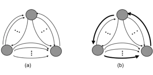
Most of the previous results on data migration assume that each disk can perform only one transfer at a time. A disk, however, may be able to handle multiple transfers simultaneously and this can reduce the total migration time significantly. For example consider Figure 2, suppose that we have three disks in the system and for each pair of nodes we haveM items to be moved and it takes one time unit to send one data item from one disk to another. Assuming that each node can participate in only one transfer, it will take3M time units. However, if a disk can perform two transfers at a time by using half of its bandwidth for each transfer, the migration can be done is2Mtime units. (It requiresM rounds but each round takes 2 time units as the bandwidth is split.)
Previous research has focused mainly on homogeneous
Fig. 2. An example of data migration when each node can handle two transfers simultaneously
storage systems, in which it is assumed that disks in a system all have the same capabilities [2], [3], [4], [5], [6], [7]. In large-scale storage systems, however, storage devices tend to have heterogeneous capabilities as devices are added over time as storage capacity demand increases. Moreover, available bandwidth of each disk can be different depending on current user traffic on different disks. That is, we may not want a disk to be involved in too many migrations if the disk is currently serving many clients. In case each disk has a different bandwidth available for migration, assuming that each node participates in only one transfer will significantly degrade the finish time of the data migration schedule as a slow node can be a bottleneck in the schedule.
here
In this paper, we consider theheterogeneous data migration problem where we will assume that each disk has different transfer constraints cv, representing how many transfers the
disk can handle simultaneously and develop algorithms to minimize the data migration time. Coffman et al. [8] con-sidered the problem and developed optimal algorithms for several special cases such as cycles, trees, and bipartite graphs. Saia [9] presented a simple1.5-approximation algorithm for arbitrary cv. The algorithm finds a solution by creating cv
copies of each node and distributing the edges incident to the node evenly. The maximum degree of the node now becomes
ddv/cve where dv is the degree of a node v. Shannon’s
theorem [10] then gives an edge coloring algorithm with at most1.5ddv/cvecolors.
We show that it is possible to find an optimal migration schedule when all cv’s are even. This can be done by
de-composing the transfer graph intomaxvddv/cvecomponents
where in each component at mostcv edges are incident tov.
For arbitrarycv, we go on to show that there is an algorithm
that uses at mostOP T+√OP T colors. This is a(1 +o(1)) -algorithm and the approximation factor is close to 1 when
OPT increases.
The remainder of this paper is organized as follows. We first describe the related work in Section II. In Section III, we formally define the problem, along with two lower bounds on the optimal solution. In Section IV, we present a polynomial time algorithm that finds an optimal migration schedule when cv’s are even. Finally, in Section V we give a (1 +o(1))
-approximation algorithm for the general case. II. RELATED WORK
Several approximation algorithms have been developed for data migration in local area networks [5], [11], [7], [12], [13], [14]. In their ground-breaking work, Hall et al. [4] studied the problem of scheduling migrations given a set of disks, with each storing a subset of items and a specified set of migrations. A crucial constraint in their problem is that each disk can participate in only one migration at a time. If both disks and data items are identical, this is exactly the problem of edge-coloring a multi-graph. That is, we can create a transfer graphG(V, E)that has a node corresponding to each disk, and a directed edge corresponding to each migration that is specified. Algorithms for edge-coloring multigraphs can now be applied to produce a migration schedule since each color class represents a matching in the graph that can be scheduled simultaneously. Computing a solution with the minimum number of colors isNP-hard [15], but several approximation algorithms are available for edge coloring [16], [17], [18], [19], [20]. With space constraints on disks, the problem becomes more challenging. Hall et al. [4] showed that with the assumption that each disk has one spare unit of space, very good constant factor approximations can be obtained. The algorithms use at most 4d∆/4e colors with at most n/3 bypass nodes,1 or at most 6d∆/4e colors without bypass nodes where∆is the maximum degree of the transfer graph andnis the number of disks.
For multi-graph edge coloring, a simple generalization of Vizing’s theorem gives a solution using at most∆ +µcolors where ∆ is the maximum degree of a node and µ is the multiplicity. Whenµ > ∆/2, a solution using 3∆/2 can be obtained [10]. The best approximation ratio for the problem have long been1.1OP T+ 0.7 [17], [19]. Recently, Sanders and Steurer obtained1 +o(1)-approximate solution. We show that when each color can be used cv times for each node
and cv are even for all v, then there is a polynomial time
algorithm to find an optimal solution. We obtain the matching approximation ratio for the general cases where each node has arbitrarycv.
Coffman et al. [8] and Sanders et al. [21] studied the problem of data migration with forwarding (data exchanged between diskiand diskjis not necessarily delivered directly fromitojbut can be forwarded over other disks). Whitehead [22] shows that when forwarding is needed because some of the edges in the transfer graph are not present in the 1A bypass node is a node that is not the target of a migration, but used as
interconnection network, then the problem is NP-complete. In this paper, we assume that transfers between disks can be done through a very fast network connection dedicated to support a storage system and any two disks can send data to each other directly.
In the data migration problem with cloning, each data item may have several copies in different disks [6], [3], [13], [11]. To handle high demand for popular items or for fault-tolerance, multiple copies may have to be created and stored on different disks [23], [24]. In the problem, each data item i initially belongs to a subset of source disksSiand needs to be moved
to another subset of destination disksDi. It is also assumed
that each data transfer takes the same amount of time and each disk can participate in only one transfer — either send or receive. The objective is to minimize the time taken to complete the migration. It is shown that this problem isNP -hard by a reduction from edge coloring and a polynomial-time algorithm with approximation factor of 9.5 is developed [6], which was further improved to 6.5 + o(1) recently [11].
Another interesting objective function in data migration is to minimize the total completion time. Minimizing the sum of weighted job completion times is one of the most common measures in the scheduling literature since it can reflect the priorities of jobs. Kim [14] developed a LP-based approximation algorithm with approximation ratio of 9, which was later improved to a 5.06-approximation by Gandhi et al. [25]. On the other hand, in a system where storage devices can be free to do other tasks as soon as their own migrations are complete, minimizing the sum of completion times over all storage devices is interesting since the performance of a device is degraded while it is involved in the migration. For the objective, Kim [14] developed 10-approximation algorithm and Gandhi et al. improved the ratio to 7.682 [26].
III. PROBLEMDEFINITION
In the HETEROGENEOUSDATAMIGRATION problem, we are given a transfer graph G = (V, E). Each node in V represents a disk in the system and each edgee = (i, j)in Erepresents a data item that need to be transferred fromito j. We assume that each data item has the same length, and therefore it takes the same amount of time for each data to migrate. Note that the resulting graph is a multi-graph as there may be several data items to be sent from diskito diskj.
We assume that each diskv can handle multiple transfers at a time. Transfer constraintcvrepresents how many parallel
data transfers the diskvcan perform simultaneously. Our objective is to minimize the number of rounds to finish all data migrations. As noted above, we assume disks send data to each other directly.
A. Lower Bounds
We have the following two lower bounds on the optimal solution. LB1 = ∆0= max v ddv/cve (1) LB2 = Γ0= max S⊆V |E(S)| b P v∈Scv 2 c (2)
whereE(S) ={(u, v)∈Es.t.u, v∈S} is the set of edges both of which endpoints are inS.
LB1 follows from the fact that for a node v, at mostcv
data items can be migrated in a round. When ∀v ∈ V, cv
is even, LB1 ≤ LB2 and, in fact, we show that there is a migration schedule that can be completed inLB1rounds. The following lemma proves that LB2 is a lower bound on the optimal solution.
Lemma 3.1: LB2is a lower bound on the optimal solution. Proof:An optimal migration is a decomposition of edges inE intoE1, E2, . . . , Ek such that for eachEi and a vertex
v, there are at mostcv edges incident tovinEi. For a subset
S⊆V, letdi(v, S)be the number of edges inEi(S)incident
tov. Then2|Ei(S)|=Pv∈Sdi(v, S). Asdi(v, S)≤cv, we
have|Ei(S)| ≤ b
P v∈Scv
2 c. AsEi’s cover all edges inE(S), the lemma follows.
IV. THECASES FOREVENTRANSFERCONSTRAINTS In this section, we describe a polynomial time algorithm to find an optimal migration schedule when each nodevhas even transfer constraintcv. We show that it is possible to obtain a
migration schedule using∆0 rounds. A. Outline of Algorithm
We first present the outline of our algorithm when cv is
even for anyv. The details of each step is given in Section IV-B.
(1) ConstructG0so that every node has degree exactlycv∆0
by adding dummy edges. (2) Find a Euler cycle (EC) onG0.
(3) Construct a bipartite graphH by considering the direc-tions of edges obtained inEC. That is, for each node v in G0, create two copies vin and vout. For an edge
e= (u, v)in G0, if the edge is visited fromu to v in EC, then create an edge from uoutto vinin H.
(4) We now decompose H into∆0 components by repeat-edly finding acv/2-matching inH.
(5) LetM1, M2, . . . , M∆0 be the matching obtained in Step (4). Then schedule one matching in each round. B. Detailed Description and Analysis
We now describe the details and show that the algorithm gives an optimal migration schedule.
Step (1)-(3): The first three steps are a generalization of Peterson’s theorem.G0 can be constructed as follows. For any node v with degree less than cv∆0, we add self-loops until
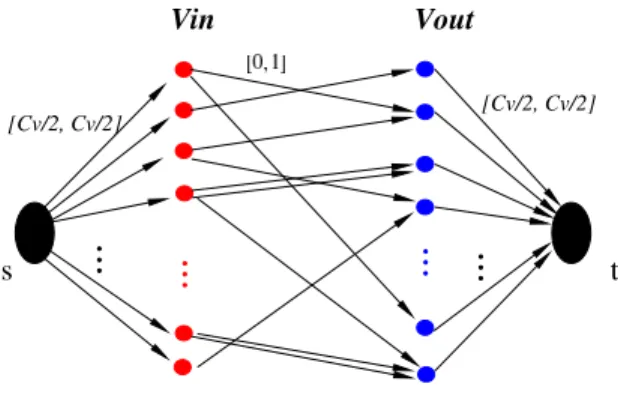
Fig. 3. Flow Network for Step (4)
the modification, the number of nodes with degree cv∆0−1
is even as cv’s are even. Pair the nodes and add edges so that
every node has degree cv∆0.
Note that each node in G0 has even degree as all cv’s are
even. Therefore, we can find a Euler cycle EC on G0. Note that for each node v, there are cv∆0/2 incoming edges and
cv∆0/2outgoing edges inEC .
We construct a bipartite graphH by considering the direc-tions of edges obtained inEC. For each nodevinG0, create two copies vinandvout. For an edgee= (u, v)inG0, if the
edge is visited from uto vin EC, then create an edge from uouttovininH. As each nodevinG0 hascv∆0/2incoming
edges andcv∆0/2 outgoing edges inEC, the degrees ofvin
andvout inH is alsocv∆0/2.
Step (4): We now find a cv/2-matching in H where exactly
cv/2edges are matched for each vin andvout. We show the
following lemma.
Lemma 4.1: There exists acv/2-matching in H and it can
be found in polynomial time.
Proof:We construct a flow network as shown in Figure 3. Create a source s and sinkt. There are edges froms to all nodesvoutand also from all nodesvintot. The capacities of
edges arecv/2. The capacities of edges fromvinandvoutare
bounded above by1and bounded below by 0.
We show that there is a fractional flow from s to t with total flow P
vcv/2. Then by the integrality theorem, we can
find an integral flow with the same total flow using, e.g., the Ford-Fulkerson algorithm.
Consider a fractional flow sending1/∆0 flow through each edge fromvouttovin. As each nodevinhascv∆0/2incoming
edges, we may sendcv/2flow tovin; this satisfies the capacity
constraints for edges from s. We can show that the capacity constraints for edges tot are also satisfied in the same way.
Since we sendcv/2for each edge from stovin, the total
isP
vcv/2. The lemma follows.
Lemma 4.2: We can decomposeH intoM1, M2, . . . , M∆0 so that eachMi is acv/2-matching in H.
Proof:Once we find acv/2-matching inH, we remove
the matched edges from H. Let M1 denote the removed matched edges. Note that in the modified H, each node has the degree exactly cv(∆0 −1)/2. Then we can show
that there is a fractional matching by sending 1/(∆0 −1) flow through each edge from vout to vin. In general, after
removingM1, M2, . . . , MifromH, each node has the degree
cv(∆0−i)/2and sending1/(∆0−i)flow through each edge
fromvout tovin gives acv/2-fractional matching. Therefore,
we can find acv/2matching in each iteration. As each node
has degree ofcv∆0/2, we can repeat this∆0 times and obtain
M1, M2, . . . , M∆0.
Step (5): Each componentMican be scheduled in one round
and therefore, we have an optimal migration schedule for even capacities.
Lemma 4.3: Each componentMi can be scheduled in one
round.
Proof: Each node v in G0 has two copies in H — vin
andvout. As vin and vout both have cv/2 edges incident to
them inMi, the total number of edges that are matched inMi
and incident tovinG0 iscv. Therefore, each componentMi
can be scheduled in one round.
Theorem 4.1: We can find an optimal migration schedule when each node has evencv.
V. GENERALCASES
In this section, we consider the case that each nodev has an arbitrarycv. The problem isNP-hard as it isNP-hard even
when cv = 1 for all nodes. We develop an algorithm that
colors edges of the given graph so that the transfer constraints cv of the nodes are satisfied. The coloring defines a data
migration schedule. As the number of colors used determines the number of rounds in our schedule, we would like our coloring algorithm to minimize the number of colors needed. We obtain an algorithm that uses at mostOP T+√OP T A. Outline of the Algorithm
We first give an overview of the coloring algorithm. Our algorithm generalizes recent work for multi-graph edge col-oring by Sanders and Steurer [20]. Our algorithm uses three particular subgraph structures, balancing orbits, color orbits and edge orbits defined in section V-B. The latter two struc-tures — color orbits and edge orbits — are generalizations of the structures used by Sanders and Steurer [20].
The algorithm starts with a naive partial coloring of G= (V, E)and proceeds in two phases. In the first phase, we use three structures and color edges until we produce a simple uncolored subgraph G0 (Section V-C1) consisting of small connected components (Section V-C2); in the second phase we colorG0 and show thatO(
p
dv(G0)/mincv)new colors
are enough to obtain a proper coloring inG0(Section V-C3). B. Preliminaries
We first introduce some definitions. Let |Ei(v)| be the
number of edges of coloriadjacent to a vertexv.
Definition 5.1 (Strongly/lightly missing color): Color c is saturatedat vertexvif|Ec(v)|=cv. The colorcismissingat
vertexvif|Ec(v)|is less thancv; in this case we distinguish
two possibilities:
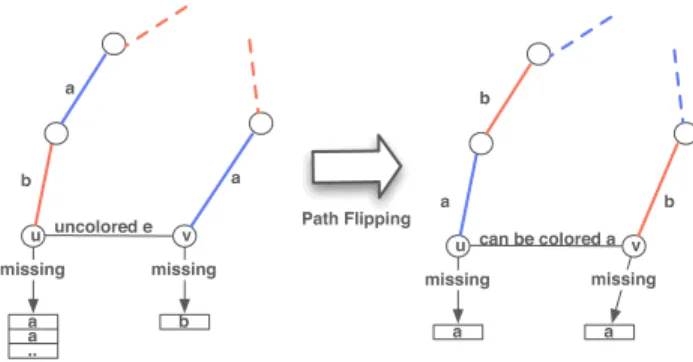
Fig. 4. ustrongly missingaand pathPends atv, we can colorewitha
• c islightly missingif|Ec(v)|=cv−1.
Definition 5.2 (alternating path): Anab-pathbetween ver-ticesu andv whereaandb are colors, is a path connecting uandvand has the following properties:
• Edges in the path have alternating colorsaandb. • Lete1= (u, w1)be the first edge on the path and suppose
e1is coloreda; thenumust be missingband not missing a.
• If v is reached, for the first time, by an edge coloredb thenvmust be missingabut not missingb; similarly, if vis reached, for the first time, by an edge coloredathen v must be missingband not missinga.
A flippingof an ab-path is a recoloring of the edges on the path such that edges previously with colorawill be recolored with colorband vice versa.
Note that unlike the case whencv= 1, an alternating path
may not be a simple path in our problem as there can be multiple edges with the same color incident to a node.
1) Balancing Orbits: We first define balancing orbits as follows.
Definition 5.3 (balancing orbit): A balancing orbitO is a node induced subgraph such that all nodesV(O)are connected by uncolored edges and the following property holds
• A vertexv∈V(O)is strongly missing a color.
The following lemma shows that if we have a balancing orbit, we can color an uncolored edge and eventually remove any balancing orbits.
Lemma 5.1: If there is a balancing orbit inG, then we can color a previously uncolored edge.
Proof:LetObe the balancing orbit. That is, a nodeu∈
V(O)is strongly missing some color. Suppose u is strongly missing color a and let e = (u, v) be the uncolored edge adjacent tou. There are three cases
• v is missing colora: in this case we can simply colore witha.
• vis missing colorband not missing colora: letP be the ab-path starting atu.P ends at a nodeu0 6=v: flipping P will makebmissing atuand thus we can colorewith b.
• P ends atv: flipping P will make amissing at v and since awas strongly missing at u,u is still missinga, so colorewitha(see Figure 4).
2) Color Orbits and Edge Orbits: In this section, we define two subgraph structures: a color orbitand anedge orbit.
Definition 5.4 (Color orbit): A color orbit O is a node induced subgraph such that all nodesV(O)are connected by uncolored edges and the following property holds
• There are at least two nodesu, v∈V(O)lightly missing the same color.
Lemma 5.2: [20] If there exists a color orbit inGthen we can color a previously uncolored edge.
By Lemma 5.1 and 5.2, whenever we find a balancing orbit or color orbit, we can color a previously uncolored edge and make progress. If neither of properties in Definition 5.3 and 5.4 hold, we callOa tight color orbit.
Our goal at the end of Phase 1 of the algorithm is to get a simple uncolored graph G0 consisting of small connected components. That is, in G0 there cannot be more than one uncolored edges between two nodes. In order to eliminate parallel uncolored edges the following subgraph structure is used.
Definition 5.5 (Lean and bad edges): If an edge e is col-ored and all its parallel edges are colcol-ored then e is a lean edge. Ifeis uncolored and has a parallel uncolored edge then eis abadedge.
Definition 5.6: An edge orbit is a subgraph consisting of two uncolored parallel edges (called theseedof the edge orbit) and then is inductively defined as follows: Let e= (x, y)be an edge in the edge orbitO, letaandbbe missing colors at xandyrespectively and letP be the alternating path starting at xthenO∪P is an edge orbit if
• no edge of color a or b is contained inO. • ∃v∈P that was not in the vertex set of O.
If edge orbitOhas a lean edge thenOis called a weak edge orbit otherwiseO is a tight edge orbit. A color c is free for an edge orbitO ifO does not contain an edge with colorc.
The following lemma from [20] states that if in some coloring of G, there exists a weak edge orbit then we make progress toward our goal of obtainingG0by either coloring a previously uncolored edge or by uncoloring a lean edge and coloring a bad edge.
Lemma 5.3: If a coloring ofG contains a weak edge orbit then we can either color a previously uncolored edge or we can uncolor a lean edge and color a bad edge.
A tight edge orbit does not have lean edges so its vertex set is connected by uncolored edges and thus a tight edge orbit is one of the following — a balancing orbit, color orbit or a tight color orbit. When it is a tight color orbit, we cannot make progress toward G0 and we call it a hard orbit. Note that no vertex in a hard orbit is strongly missing a color, no
two nodes are lightly missing the same color, and no edge in a hard orbit is lean.
3) Growing Orbits: A color c is full in a hard orbit O if c is saturated on all vertices of V(O) but at most one vertex in V(O) is lightly missing c or equivalently if
|Ec(v)∩E(V(O))| ≥ b
P v∈V(O)cv
2 c.So if colorcis full in a hard orbitOit cannot be used to color uncolored edges whose endpoints are inO.
Definition 5.7 (Lower bound witnesses): A hard orbit is a
∆0-witness if all missing colors at some node are non-free. It is aΓ0-witness if all free colors of the orbit are full.
The intuition behind the witnesses is the following. Suppose very few colors are used in hard orbit O, in the case of
Γ0-witness almost all color classes are full in O and in the case of a ∆0-witness almost all available colors are strong on some node v ∈ V(O). So a witness in some coloring using q colors indicates that it is almost impossible to color an additional uncolored edge using the availableq colors and thus the number of available colors needs to be increased.
Lemma 5.4: [20] Given a hard orbit in some coloring we can either find a witness or compute a larger edge orbit. C. Algorithm
The algorithm proceeds in two phases. The outcome of the first phase would be G0, a simple uncolored graph with no large components. The following procedure for the first phase eliminates all the bad edges inG(Section V-C1) and reduces the size of connected components (Section V-C2), which gives G0 with the desired properties. In the second phase (Section V-C3), we color the remaining subgraphG0.
1) Eliminating bad edges: Given a partial coloring usingq colors, we iterate over a list of bad edges and we execute the following steps.Given an edge orbitO
(1) If nodes of O form a balancing or color orbit, apply Lemma 5.1 or 5.2.
(2) IfOis weak, apply Lemma 5.3. (3) IfOis a hard orbit, apply Lemma 5.4.
a) If Lemma 5.4 gives a larger edge orbit O∪P, repeat withO=O∪P.
b) If Lemma 5.4 gives a witness then increase q by one color and color the bad edges in the seed with the additional color.
The output of this procedure is a simple subgraph G0 of G induced by uncolored edges. In Lemma 5.5 and Lemma 5.6, we show an upper bound on the number of used colors if there is a∆0 orΓ0-witness. The next procedure reduces the size of the connected components ofG0 whenever G0 has balancing or color orbits.
2) Reducing size of connected components: For every con-nected componentU ofG0,
1) If U contains a vertex that is strongly missing a color then use Lemma 5.1 to color an uncolored edge. 2) If U contains two or more vertices that are lightly
missing the same color use Lemma 5.2 to color an uncolored edge.
So at the end of the first phase we have the simple subgraph G0where for every connected componentUofG0, no vertex is strongly missing a color and no two vertices ofU miss the same color. In Lemma 5.7, we show that the size ofG0is no more than q−q∆+20+2.
3) Coloring G0: Phase 2 colors G0. We use only
maxvd dv(G0)
cv e+ 1colors. The procedure goes as follows: 1) Createcvcopies of each vertexvand distribute the edges
over the copies so that each vertex is adjacent to at most
ddv(G0)
cv eedges where dv(G0)represents the degree of v inG0.
2) Use Vizing’s algorithm to properly color each compo-nent. We need at mostmaxvddv(cGv0)e+ 1 colors.
3) Contract the copies back to v getting a coloring where for any node v there is no more than cv edges of the
same color. D. Analysis
In the following q denotes the total number of colors available for the algorithm. We show that the algorithm colors all the edges of G using at most q = OP T + Θ(√OP T)
colors. We first bound the number of used colors when there is a∆0 orΓ0-witness.
Lemma 5.5: Let O be a hard orbit. If O is a ∆0-witness thenq≤∆0+2|V(cO−)|−4 where c
−= min
v∈V(O)cv.
Proof:For a trivial edge orbit allqcolors are free. Other edge orbits are constructed by adding an alternating path with new colors to another edge orbit. Every path adds at least a new node to the edge orbit and reduces the number of free colors by at most2. So the total number of free colors for an edge orbit is at leastq−2(|V(O)| −2).
IfO is a∆0-witness then some nodeu∈V(O)misses no free color. Since u is not strongly missing any color and is incident to at least two uncolored edges, the number of missing colors for u is at least cuq−du+ 2. As the number of free
colors and missing colors ofuare disjoint then q−2|V(O)|+ 4 +cuq−du+ 2 ≤ q
cuq ≤ du+ 2|V(O)| −6
q ≤ ∆0+2|V(O)| −4
c− Lemma 5.6: Let O be a hard orbit. If O is a Γ0-witness thenq≤Γ0+ 2|V(O)| −4− 2
c+.
Proof:IfO is aΓ0-witness then all free colors ofOare full. SinceOis a hard orbit there is at most|E(V(O))−V(O)|
colored edges between vertices inV(O). So the number of full colors is at most |E(V(O))−V(O)| b P v∈V(O)cv 2 c ≤Γ0− V(O) b P v∈V(O)cv 2 c . Let c+ = max
v∈V(O)cv. Then the number of full colors is
at most Γ0−2/c+. As the total number of free colors for an edge orbit is at leastq−2(|V(O)| −2), the lemma follows.
We now bound the size ofG0.
Lemma 5.7: Let O be a tight color orbit. Then |V(O)| ≤
q+2
q−∆0+2.
Proof:Since no two nodes inV(O)share a missing color, the number of missing colors at the nodes ofO is less than q. Every node u in V(O) misses at least cuq −du(≥ q−
∆0)colors as no node in V(O)is strongly missing a color. The uncolored edge adjacent to a node u ∈ V(O) implies an additional color is missing atu. As there are |V(O)| −1
uncolored edges inOthere are at least2(|V(O)|−1)additional colors missing at nodes inV(O). Thus we have
|V(O)|(q−∆0) + 2(|V(O)| −1)≤q ,
q|V(O)| −∆0|V(O)|+ 2(|V(O)| −1)≤q ,and thus
|V(O)| ≤ q+ 2
q−∆0+ 2.
Corollary 5.1: Ifq = b(1 +)∆0c −1, the size of a hard orbitOis at most1 +1.
Proof:A hard orbit is also a tight color orbit and thus
|V(O)| ≤ q+ 2 q−∆0+ 2 ≤1 + ∆0 b∆0c+ 1≤1 + 1 . The following corollary follows from Lemma 5.5, 5.6, and Corollary 5.1,
Corollary 5.2: Ifq=b(1 +)∆0c −1and there is a witness thenq≤OP T+ 2−2
The following lemma provides a bound on the number of required colors forG0.
Lemma 5.8: Suppose that the size of the largest component ofG0 is bounded by C. Then coloring G0 requires at most
dC−1
c− e+ 1colors.
Proof: By Vizing’s theorem for simple graphs, at most
maxddv(G0)
cv e+ 1 new colors will be used in Phase 2 as described in Section V-C3. This procedure colors G0 using at mostdC−1
c− e+ 1asdv(G0)≤C−1.
Theorem 5.1: Given a transfer graph G, we can compute a coloring of the edges using at most OP T+O
√ OP T
colors.
Proof:We start our coloring algorithm withb(1+)∆0c−
1colors. At the end of Phase 1, all edges that remain uncolored create a simple subgraph G0 (a collection of hard orbits). Furthermore, the number of colors has increased only if there was a witness. By Corollary 5.2, the number of colors used is at mostOP T+2−2. Thus at the end of phase 1, at most
max(b(1 +)∆0c −1, OP T+2
−2)colors have been used. In
Phase 2, the algorithm colors the connected components ofG0 which are hard orbits. By Corollary 5.1 their size is at most
1 + 1/.G0 is a simple graph and has degree no more than
1/thus the algorithm in Section V-C3 yields a coloring ofG0 using at most1 + 1/(·c−)additional colors by Lemma 5.8. So the total number of colors used in the coloring algorithm is at most the maximum ofb(1+)∆0c+c1−, OP T+2−c1−−1). Choosing=
√ 2 √
OP T gives the theorem.
We start with∆0+√∆0 colors and proceed as described in Section V-C. The overall running time of the algorithm is O(|E|√∆0(∆ +|V|))by lemma 5.9
Corollary 5.3: The coloring algorithm uses at mostOP T+
O(√OP T)colors, which implies an approximation factor of
1 +o(1)asOP T increases.
Lemma 5.9: Let C be such that no connected component ofG0has size exceedingC, then the runtime of the algorithm is
O(|E|C(∆ +|V|))
Proof: As the size of connected components of G0 is less than C, the missing colors at each node of G0 can be determined in O(C∆). Flipping a path can be done in time proportional to the number of vertices on that path, so at most V. This is iterated at mostCtimes inG0. So the total time for Lemmas 5.1, 5.2 and 5.3 isO(C(|V|+ ∆)). Thus the first2
steps of procedure V-C1 and procedure V-C2 areO(C(|V|+ ∆)). Step 3(b) of procedure V-C1 is done in constant time and in step 3(a)O(∆ +|V|)steps are needed to grow a hard orbit (Lemma 5.4). As we iterate over all bad edges the overall runtime of the algorithm isO(|E|C(∆ +|V|))
Note that the running time of the algorithm described above is polynomial in |E|,|V| and ∆. The authors in [20] develop a solution exploiting that a graph with even edge multiplicities can be colored by coloring a graph with halved edge multiplicities and then using each color twice. The same transformation applies to the above algorithm to make it polynomial in|V|and in the number of bits needed to encode edge multiplicities.
VI. Conclusion
In this paper, we consider the data migration problem where each storage node has different transfer constraint cv,
representing how many transfers the node can simultaneously handle. Our objective is to minimize the data migration time. We show that it is possible to find an optimal migration schedule when cv is even for all v. For the general case,
we formulate the problem as a variant of multi-edge coloring problem in which each color can be usedcv times at nodev.
Furthermore, though the problem isNP-hard, we give an effi-cient algorithm that offers a rigorous(1+o(1))-approximation guarantee.
REFERENCES
[1] H. Tang and T. Yang, “An efficient data location protocol for self-organizing storage clusters,” inProceedings of the International Con-ference for High Performance Computing and Communications (SC), 2003.
[2] E. Anderson, J. Hall, J. Hartline, M. Hobbes, A. Karlin, J. Saia, R. Swaminathan, and J. Wilkes, “An experimental study of data mi-gration algorithms,” inWorkshop on Algorithm Engineering, 2001. [3] L. Golubchik, S. Khuller, Y. Kim, S. Shargorodskaya, and Y. J. Wan,
“Data migration on parallel disks,” in12th Annual European Symposium on Algorithms (ESA), 2004.
[4] J. Hall, J. Hartline, A. Karlin, J. Saia, and J. Wilkes, “On algorithms for efficient data migration,” inSODA, 2001, pp. 620–629.
[5] S. Kashyap, S. Khuller, Y.-C. Wan, and L. Golubchik, “Fast reconfigu-ration of data placement in parallel disks,” inALENEX, 2006.
[6] S. Khuller, Y. Kim, and Y.-C. Wan, “Algorithms for data migration with cloning,” in22nd ACM Symposium on Principles of Database Systems (PODS), 2003, pp. 27–36.
[7] B. Seo and R. Zimmermann, “Efficient disk replacement and data migration algorithms for large disk subsystems,”ACM Transactions on Storage Journal (TOS), vol. 1, no. 3, pp. 316–345, AUG 2005. [8] E. Coffman, M. G. Jr., D. Johnson, and A. Lapaugh, “Scheduling file
transfers,”SIAM J. Computing, vol. 14, no. 3, pp. 744–780, 1985. [9] J. Saia, “Data migration with edge capacities and machine speeds,”
University of Washington, Tech. Rep., 2001. [Online]. Available: citeseer.ifi.unizh.ch/article/saia01data.html
[10] C. Shannon, “A theorem on colouring lines of a network,” J. Math. Phys., vol. 28, pp. 148–151, 1949.
[11] S. Khuller, Y. Kim, and A. Malekian, “Improved algorithms for data migration,” inAPPROX, 2006.
[12] C. Lu, G. Alvarez, and J. Wilkes, “Aqueduct:online data migration with performance guarantees,” inProceedings of the Conference on File and Storage Technologies, 2002.
[13] S. Khuller, Y.-A. Kim, and Y.-C. J. Wan, “On generalized gossiping and broadcasting,” in12th Annual European Symposium on Algorithms, 2004.
[14] Y.-A. Kim, “Data migration to minimize the average completion time,” J. of Algorithms, vol. 55, 2005.
[15] I. Holyer, “The np-completeness of edge-coloring,”SIAM J. on Com-puting, vol. 10, no. 4, 1981.
[16] D. Hochbaum, T. Nishizeki, and D.B.Shmoys, “Better than “best pos-sible” algorithm to edge color multigraphs,” J. of Algorithms, vol. 7, no. 1, 1986.
[17] T. Nishizeki and K. Kashiwagi, “On the 1.1 edge-coloring of multi-graphs,”SIAM J. on Discrete Math., vol. 3, 1990.
[18] M. Goldberg, “Edge-colorings of multigraphs: Recoloring techniques,” Journal of Graph Theory, vol. 8, pp. 122–136, 1984.
[19] A. Caprara and R. Rizzi, “Improving a family of approximation al-gorithms to edge color multi-graphs,”Information Processing Letters, vol. 68, pp. 11–15, 1998.
[20] P. Sanders and D. Steurer, “An asymptotic approximation scheme for multigraph edge coloring,” inSODA ’05: Proceedings of the sixteenth annual ACM-SIAM symposium on Discrete algorithms. Philadelphia, PA, USA: Society for Industrial and Applied Mathematics, 2005, pp. 897–906.
[21] P. Sanders and R. Solis-Oba, “How helpers hastenh-relations,”Journal of Algorithms, vol. 41, pp. 86–98, 2001.
[22] J. Whitehead, “The complexity of file transfer scheduling with forward-ing,”SIAM J. Comput., vol. 19, no. 2, pp. 222–245, 1990.
[23] S. Berson, S. Ghandeharizadeh, R. Muntz, and X. Ju, “Staggered striping in multimedia information systems,” in ACM SIGMOD International Conference on Management of Data, 1994, pp. 79–90. [Online]. Available: citeseer.ist.psu.edu/berson93staggered.html [24] M. Stonebraker, “The case for shared nothing,”Database Engineering
Bulletin, vol. 9, no. 1, pp. 4–9, 1986. [Online]. Available: citeseer.ist.psu.edu/stonebraker86case.html
[25] R. Gandhi, M. M. Halld´orsson, G. Kortsarz, and H. Shachnai, “Improved results for data migration and open shop scheduling,” inICALP, 2004, pp. 658–669.
[26] R. Gandhi, M. Halld´orsson, G. Kortsarz, and H. Shachnai, “Improved bounds for sum multicoloring and scheduling dependent jobs with minsum criteria,” inWAOA, 2004, pp. 68–82.