Using a mobile phone acceleration sensor in physics experiments on free
and damped harmonic oscillations
Juan Carlos Castro-Palacio, Luisberis Velázquez-Abad, Marcos H. Giménez, and Juan A. Monsoriu
Citation: Am. J. Phys. 81, 472 (2013); doi: 10.1119/1.4793438
View online: http://dx.doi.org/10.1119/1.4793438
View Table of Contents: http://ajp.aapt.org/resource/1/AJPIAS/v81/i6
Published by the American Association of Physics Teachers
Additional information on Am. J. Phys.
Journal Homepage: http://ajp.aapt.org/
Journal Information: http://ajp.aapt.org/about/about_the_journal
Top downloads: http://ajp.aapt.org/most_downloaded
APPARATUS AND DEMONSTRATION NOTES
The downloaded PDF for any Note in this section contains all the Notes in this section.
Frank L. H. Wolfs,Editor
Department of Physics and Astronomy, University of Rochester, Rochester, New York 14627
This department welcomes brief communications reporting new demonstrations, laboratory equip-ment, techniques, or materials of interest to teachers of physics. Notes on new applications of older apparatus, measurements supplementing data supplied by manufacturers, information which, while not new, is not generally known, procurement information, and news about apparatus under development may be suitable for publication in this section. Neither theAmerican Journal of Physicsnor the Editors assume responsibility for the correctness of the information presented.
Manuscripts should be submitted using the web-based system that can be accessed via theAmerican Journal of Physicshome page, http://ajp.dickinson.edu and will be forwarded to the ADN editor for consideration.
Using a mobile phone acceleration sensor in physics experiments
on free and damped harmonic oscillations
Juan Carlos Castro-Palacio
Departamento de Fısica, Universidad de Pinar del Rıo. Martı 270, Esq. 27 de Noviembre, 20100 Pinar del Rıo, Cuba
Luisberis Velazquez-Abad
Departamento de Fısica, Universidad Catolica del Norte. Av. Angamos 0610 Antofagasta, Chile
Marcos H. Gimenez
Departamento de Fısica Aplicada, Universitat Polite`cnica de Vale`ncia. Camı de Vera s/n, 46022 Vale`ncia, Spain
Juan A. Monsoriua)
Centro de Tecnologıas Fısicas, Universitat Polite`cnica de Vale`ncia, Camı de Vera s/n, 46022 Vale`ncia, Spain
(Received 9 November 2012; accepted 11 February 2013)
We have used a mobile phone acceleration sensor, and the Accelerometer Monitor application for Android, to collect data in physics experiments on free and damped oscillations. Results for the period, frequency, spring constant, and damping constant agree very well with measurements obtained by other methods. These widely available sensors are likely to find increased use in instructional laboratories.VC2013 American Association of Physics Teachers.
[http://dx.doi.org/10.1119/1.4793438]
I. INTRODUCTION
Electronic portable or everyday-use devices offer new opportunities for the physics laboratory at all teaching lev-els. This has been the case for digital cameras,1webcams,2 the optical mouse of computers,3,4XBee transducers,5 wii-mote,6 and other game console controllers.7 For instance, digital camera techniques have been widely used to visual-ize physics concepts.8–11 Analysis of digitally recorded video can also yield measurements of distances, time inter-vals, and trajectories of objects, facilitating students’ com-prehension of otherwise abstract concepts. As another example, the wiimote6,12,13 has a three-axis accelerometer which communicates with the game console via Bluetooth. The use of accelerometers in the physics laboratory has been described by Weltin14and Hunt.15,16
Although the wiimote provides a low-cost way to track motion in a variety of physics experiments,17it is not a com-mon device in physics laboratories. In this paper, we study the possibility of using another accelerometer-equipped device, which almost all students have with them, although
they may not realize it. We use a mobile phone acceleration sensor to study free and damped oscillations of a glider on an air track. Mechanical oscillation is an important topic in
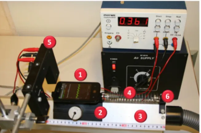
Fig. 1. Photograph of the experimental setup showing (1) smart phone, (2) glider, (3) air track, (4) spring, (5) photometer, and (6) the fixed end.
most undergraduate physics programs, and many authors have suggested laboratory exercises on this topic.18,19 The air track is a useful device for such exercises because the friction force can be easily decreased.20Although the use of an air track and glider is traditional, we are not aware of others who have used a mobile phone as an accelerometer in such an experiment.
In this paper, we will first describe the experimental setup and the features of our software, the Acceleration Monitor mobile application. We will then present results for free harmonic oscillations, followed by results for damped oscillations.
II. EXPERIMENTAL SETUP
A photograph of the experimental setup is shown in Fig.1. The mobile phone is placed on a glider, which rests on the air track and is connected to a fixed end by a spring. While the air is flowing, the glider can oscillate almost freely after receiving a push. The mobile phone used in our experiments was a model LG-E510 running Android version 2.3.4. This phone’s mass is 124.0 g and the glider’s mass is 180.6 g. The mass of the glider can be changed by adding weights at both sides, thus changing the frequency of oscillation.
To collect data from the mobile sensor, we used the free Android application Accelerometer Monitor, version 1.5.0, which can be downloaded from the Google Play web site.21 The application reports the three components of the phone’s acceleration at regularly spaced time intervals. The effect of gravity can be removed from the data. The precision in the measurement of the acceleration is da¼0:01197 m=s2 and
the average time step is dt¼0:02 s. Since the oscillations take place along theyaxis, the values of the acceleration for thexandzaxes remain very close to zero. This application also allows saving the output data to a file, from which the data can be used for further analysis.
Fig. 2. Close-up of the mobile phone screen showing an acceleration graph for free oscillations.
Fig. 3. A fragment of the output data file of the Accelerometer Monitor application. The first three columns give the three acceleration components while the fourth column gives the elapsed time between measurements.
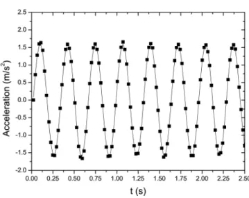
Fig. 4. As an example of the experimental acceleration data (squares) and fitted curve (solid line) for mass 3.
Table I. Parameters and their errors from fitting the acceleration data for free oscillations. m60.0001 (kg) A6dAðm=s2Þ x06dx0 (rad/s) /06d/0 (rad) R2 m1 0.3045 1.08260.008 24.74760.010 0.79760.015 0.9938 m2 0.4043 1.20460.006 21.54660.005 2.47960.009 0.9968 m3 0.5004 1.59860.006 19.40860.004 0.37760.007 0.9984 m4 0.6084 1.17160.007 17.66960.006 0.39760.011 0.9953 m5 0.6285 0.85660.007 17.37160.006 2.55360.016 0.9875 m6 0.6961 1.54260.008 16.52660.007 2.83060.011 0.9966
Table II. Comparison of periods calculated from the fit to accelerometer data (column 2) and obtained with a separate photometer measurement (col-umn 3). The fourth col(col-umn shows the percentage difference.
Tfit6dTfit(s) Tphoto60:001 (s) Diff. (%)
m1 0.253960.0001 0.259 1.99 m2 0.291660.0001 0.291 0.21 m3 0.323760.0001 0.323 0.23 m4 0.355660.0001 0.356 0.11 m5 0.361760.0001 0.365 0.91 m6 0.380260.0002 0.380 0.05
Once the application has been downloaded to the mobile device, a simple test can be performed to check for correct functioning. If the phone is left quiet on a horizontal surface, the application output curves for the acceleration should indicate values very close to zero for all axes.
For the case of damped oscillations, some dissipation of the amplitude of the oscillations can be obtained by slowing the air flow to the air track.
III. FREE HARMONIC OSCILLATIONS
Figure 2shows the screen of the Accelerometer Monitor application during free harmonic motion, with negligible friction. The acceleration is accurately modeled by a sinusoi-dal function of time, so we fit the data to the formula,
aðtÞ ¼Asinðx0tþ/0Þ; (1)
whereAis the acceleration amplitude,x0is the angular
fre-quency, and/0is the phase constant.
In order to start the oscillations in the system, the glider with the mobile was pulled to the right and then released. We collected data for six different glider masses, obtained by adding weights to both sides of the glider. Figure3shows a portion of the text output from the Accelerometer Monitor application, with header data and then a long data list, with columns for each of the three acceleration components and the time interval between measurements. We used a least-squares fit to determine the three parametersA,x0, and/0,
from these data.
The scatter of the data points and the fitted curve are shown in Fig.4. TableIshows the parameters and their errors from fitting to Eq.(1). The quality of the fit can be seen in the val-ues of the regression coefficientR2, always close to 1.
Table II compares the period of oscillation, calculated from the fitted frequency, to a separate measurement of the period obtained directly from a photometer. In most cases, the discrepancies are less than 1%.
Once the values of the mass (m) and the frequency of the free oscillations (x0) have been obtained, the spring constant
kfit can be calculated. To do so, we have carried out a
least-squares linear regression to fit the equation x2
0¼kfit=m,
using the values shown in TableIII. We also made a separate measurement of the spring constant by hanging a 500 g mass from the spring and measuring the static shift in the position. A comparison of the two results forkis shown in TableIV.
IV. DAMPED HARMONIC OSCILLATIONS
By reducing the air flow in the air track, we can introduce significant friction and study damped oscillations. Figure 5
shows the screen of the mobile phone after a series of damped oscillations. Assuming linear damping for simplic-ity, we can fit the acceleration data to the formula,
aðtÞ ¼Dectsinðxtþ/Þ; (2) Table III. Data for the calculation of the spring constant.
m16dm1ðkg1Þ x2 06dx20ðrad2=s2Þ m1 3.284160.0011 612.460.5 m2 2.473460.0006 464.260.2 m3 1.998460.0004 376.760.1 m4 1.643760.0003 312.260.2 m5 1.591160.0003 301.860.2 m6 1.436660.0002 273.160.2
Table IV. Comparison of results for the measured spring constant: from a fit to the accelerometer results, by hanging a static weight, and the percent difference.
From the fit With static weight
kfit6dkfit(N/m) k6dk(N/m) Diff. (%)
187.960.6 18967 0.58
Fig. 5. Photograph of the smart phone displaying an acceleration graph for the case of damped oscillations.
Fig. 6. Experimental acceleration data (squares) and fitted curve (solid line) for damped oscillations.
Table V. Parameters and their errors from fitting the acceleration data for damped oscillations.
D6dDðm=s2Þ c6dcðs1Þ x6dx(rad/s) /6d/(rad) R2 m6 1.6460.02 0.5860.02 16.5260.01 0.5660.01 0.9816
whereDis the initial acceleration amplitude,cis the linear damping constant, and/is a phase constant. Figure6shows a fit of the data to this formula, while TableVshows the pa-rameters obtained from the fit.
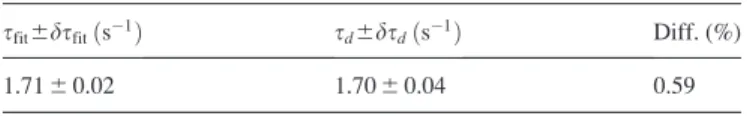
The relaxation time,s, is the inverse of the damping con-stant:s¼1=c. It can also be derived from the formula,
s¼TdTfit 2p 1 ðT2 dT 2 fitÞ 1=2; (3)
whereTfitis the period of the free oscillations (see TableII)
andTd ¼2p=xis the period of the damped oscillations. In
Table VI, we compare the values of the relaxation time obtained from each of these formulas.
V. CONCLUSIONS
We have studied free and damped oscillations in a very simple way using a mobile phone acceleration sensor and the free Accelerometer Monitor application for the Android operating system. Results for the period, frequency, and spring constant are in good agreement with more traditional measurements of these quantities. We have also studied damped oscillations and obtained consistent results for the effective linear damping constant. The success of these measurements demonstrates the feasibility of using a mobile phone acceleration sensor in the general physics laboratory. For example, the mobile phone accelerometer could also be used to study two-dimensional motions on an air table22and various types of pendulum motions.
ACKNOWLEDGMENTS
The authors would like to thank the Institute of Education Sciences, Universitat Polite`cnica de Vale`ncia (Spain), for the support of the Teaching Innovation Group, MoMa.
a)
Electronic mail: [email protected]
1
J. A. Monsoriu, M. H. Gimenez, J. Riera, and A. Vidaurre, “Measuring coupled oscillations using an automated video analysis technique based on image recognition,”Eur. J. Phys.26, 1149–1155 (2005).
2
S. Shamim, W. Zia, and M. S. Anwar, “Investigating viscous damping using a webcam,”Am. J. Phys.78, 433–436 (2010).
3O. R. Ochoa and N. F. Kolp, “The computer mouse as a data acquisition
interface: Application to harmonic oscillators,”Am. J. Phys.65, 1115– 1118 (1997).
4
T. W. Ng and K. T. Ang, “The optical mouse for harmonic oscillator experimentation,”Am. J. Phys.73, 793–795 (2005).
5E. Ayars and E. Lai, “Using XBee transducers for wireless data collection,”
Am. J. Phys.78, 778–781 (2010).
6
S. L. Tomarkenet al., “Motion tracking in undergraduate physics laborato-ries with the Wii remote,”Am. J. Phys.80, 351–354 (2012).
7M. Vannoni and S. Straulino, “Low-cost accelerometers for physics
experiments,”Eur. J. Phys.28, 781–787 (2007).
8
A. Vidaurre, J. Riera, M. H. Gimenez, and J. A. Monsoriu, “Contribution of digital simulation in visualizing physics processes,”Comp. Appl. Eng. Educ.10, 45–49 (2002).
9
J. Riera, M. H. Gimenez, A. Vidaurre, and J. A. Monsoriu, “Digital simulation of wave motion,” Comp. Appl. Eng. Educ. 10, 161–166 (2002).
10H. C. Chung, J. Liang, S. Kushiyama, and M. Shinozuka, “Digital image
processing for non-linear systems identification,”Int. J. Non-Linear Mech.
39, 691–707 (2004).
11
T. Greczylo and E. Debowska, “Using a digital video camera to examine coupled oscillations,”Eur. J. Phys.23, 441–447 (2002).
12
A. Kawam and M. Kouh, “Wiimote experiments: 3-D inclined plane problem for reinforcing the vector concept,”Phys. Teach.49, 508–612 (2011).
13R. Ochoa, F. G. Rooney, and W. J. Somers, “Using the wiimote in
intro-ductory physics experiments,”Phys. Teach.49, 16–18 (2011).
14
H. Weltin, “Accelerometer,”Am. J. Phys.34, 825–826 (1966).
15J. L. Hunt, “Forced and damped harmonic oscillator experiment using an
accelerometer,”Am. J. Phys.53, 278–279 (1985).
16
J. L. Hunt, “Accurate experiment for measuring the ratio of specific heats of gases using an accelerometer,” Am. J. Phys. 53, 696–697 (1985).
17A. Skeffington and K. Scully, “Simultaneous tracking of multiple points
using a wiimote,”Phys. Teach.50, 482–484 (2012).
18
P. Onorato, D. Mascoli, and A. De Ambrosis, “Damped oscillations and equilibrium in a mass-spring system subject to sliding friction forces: Integrating experimental and theoretical analyses,”Am. J. Phys.78, 1120– 1127 (2010).
19
G. Flores-Hidalgo and F. A. Barone, “The one-dimensional damped forced harmonic oscillator revisited,”Eur. J. Phys.32, 377–379 (2011).
20J. Berger, “On potential energy, its force field and their measurement
along an air track,”Eur. J. Phys.9, 47–50 (1988).
21
<https://play.google.com/store/apps>.
22N. C. Bobillo-Ares and J. Fernandez-Nufiez, “Two-dimensional harmonic
oscillator on an air table,”Eur. J. Phys.16, 223–227 (1995). Table VI. Comparison of the relaxation time obtained from the measured
damping constant,sfit¼1=c, with the relaxation timesdobtained from Eq. (3).
sfit6dsfitðs1Þ sd6dsdðs1Þ Diff. (%)
1.7160.02 1.7060.04 0.59