HAL Id: hal-01958835
https://hal.archives-ouvertes.fr/hal-01958835v2
Submitted on 7 Jan 2020
HAL is a multi-disciplinary open access archive for the deposit and dissemination of sci-entific research documents, whether they are pub-lished or not. The documents may come from teaching and research institutions in France or
L’archive ouverte pluridisciplinaire HAL, est destinée au dépôt et à la diffusion de documents scientifiques de niveau recherche, publiés ou non, émanant des établissements d’enseignement et de recherche français ou étrangers, des laboratoires
Logistic Regression with Missing Covariates –
Parameter Estimation, Model Selection and Prediction
Wei Jiang, Julie Josse, Marc Lavielle
To cite this version:
Wei Jiang, Julie Josse, Marc Lavielle. Logistic Regression with Missing Covariates – Parameter Estimation, Model Selection and Prediction. Computational Statistics and Data Analysis, Elsevier, In press, pp.106907. �10.1016/j.csda.2019.106907�. �hal-01958835v2�
Logistic Regression with Missing Covariates – Parameter
Estimation, Model Selection and Prediction within a
Joint-Modeling Framework
Wei Jianga,∗, Julie Jossea, Marc Laviellea, TraumaBase Groupb
aInria XPOP and CMAP, ´Ecole Polytechnique, France bHˆopital Beaujon, APHP, France
Abstract
Logistic regression is a common classification method in supervised learning. Surprisingly, there are very few solutions for performing logistic regression with missing values in the covariates. A complete approach based on a stochastic approximation version of the EM algorithm is proposed in order to perform statistical inference with missing values, including the estimation of the parameters and their variance, derivation of confidence intervals, and also a model selection procedure. The problem of prediction for new observations on a test set with missing covariate data is also tackled. Supported by a simulation study in which the method is compared to previous ones, it has proved to be computationally efficient, and has good coverage and variable selection properties. The approach is then illustrated on a dataset of severely traumatized patients from Paris hospitals by predicting the occurrence of hemorrhagic shock, a leading cause of early preventable death in severe trauma cases. The aim is to improve the current red flag procedure, a binary alert identifying patients with a high risk of severe hemorrhage. The method is implemented in the R packagemisaem.
Keywords: incomplete data, observed likelihood, Metropolis-Hastings, public health
1. Introduction
Missing data exist in almost all areas of empirical research. There are various reasons why it may occur, including survey non-response, unavailability of measurements, and lost data. One popular approach to handle missing values consists in modifying estimation processes so that they can be applied to incomplete data. For example, one can use the EM algorithm [1] to obtain the maximum likelihood estimate (MLE) despite missing values, accompanied by a supplemented EM algorithm (SEM) [2] or Louis’ formula [3] for estimating the variance. This strategy is valid under missing-at-random (MAR) mechanisms [4, 5] in which data missingness is independent of the missing values, given the observed data. Even
∗Corresponding author
though this approach is perfectly suited to specific inference problems with missing values, there are few solutions or implementations available, even for simple models such as logistic regression, the focus of this paper.
One explanation is that the expectation step of the EM algorithm often involves unfea-sible computations. In the framework of generalized linear models, Ibrahim et al. [6,7] have suggested using a Monte Carlo EM (MCEM) algorithm [8, 9], replacing the integral by its empirical sum using Monte Carlo sampling. Ibrahim et al. [6] also estimated the variance using a Monte Carlo version of Louis’ formula, involving Gibbs sampling with an adaptive rejection sampling scheme [10]. However, their approach has a high computational cost and was only implemented for monotone patterns of missing values and for missing values in only two variables in a dataset.
In this paper, we develop a stochastic approximation version of the EM algorithm (SAEM) [11], based on Metropolis-Hastings sampling, to perform statistical inference for logistic regression with incomplete data, where the missing data is found anywhere in the covariates. SAEM uses a stochastic approximation procedure to estimate the conditional expectation of the complete-data likelihood, instead of generating a large number of Monte Carlo samples, which lead to an undeniable computational advantage over MCEM, which we illustrate in the simulations. In addition, SAEM allows for model selection using a criterion based on a penalized version of the observed-data likelihood. This is very useful in prac-tice, as few methods are available to select models when there are missing values. Of those that do exist, Claeskens and Consentino [12], Consentino and Claeskens [13] suggested an approximation of AIC, Jiang et al. [14] defined generalized information criteria, and—in the imputation framework—Liu et al. [15] proposed combining penalized regression techniques with multiple imputation and stability selection. As well as aiming to maximize the MLE for observed data, Chow [16], Yuen Fung and A. Wrobel [17] also studied the linear discrim-inant function for logistic regression, using pairs of observed values in different columns to calculate the covariance matrix. Note that another solution is to use a Laplace approxima-tion to compute integrals; this linearizes the likelihood funcapproxima-tion via differentiaapproxima-tion, whereas SAEM supports likelihood-based inference without the intermediate step.
This paper proceeds as follows: In Section2we describe the motivation for the work: the TraumaBase1 project involving a French multicenter prospective trauma registry. Section 3
provided the assumptions and notation used throughout the paper. In Section 4, we derive a SAEM algorithm to obtain the maximum likelihood estimate of parameters in a logistic regression model for continuous covariate data, under the MAR mechanism of missing data. Following parameter estimation, we show how to estimate the Fisher information matrix using a Monte Carlo version of Louis’ formula. Section 5 describes the model selection scheme, based on a Bayesian information criterion (BIC) with missing values. In addition, we propose an approach to perform prediction for a new observation that includes missing values. Section 6 presents a simulation study where the proposed approach is compared to methods such as multiple imputation [18] with respect to bias, coverage, and execution time. In Section 7, we apply the newly developed approach to predict the occurrence of
1
hemorrhagic shock in patients with blunt trauma in the TraumaBase dataset, where it is crucial to efficiently manage missing data because the percentage of it varies from 0 to 60% depending on the variable. Predictions made using SAEM show an improvement over those made by emergency doctors. Lastly, Section8discusses the results and provides conclusions. Our contribution is to give users the ability to perform logistic regression with missing values within a joint-modeling framework, one that combines computational efficiency and a sound theoretical foundation. The methods presented in this article are implemented as an R [19] package misaem [20], available on CRAN. The code to reproduce all simulations can be found on GitHub [21].
2. Medical emergencies
Our work is motivated by a collaboration with the TraumaBase group at APHP (Public Assistance - Hospitals of Paris), which is dedicated to the management of severely trauma-tized patients.
Major trauma refers to injuries that cause prolonged disability or endanger a person’s life. The World Health Organization has recently reported that major trauma, such as from road accidents, interpersonal violence and falls, is a prominent source of mortality and morbidity around the world [22]. In particular, major trauma is the leading cause of mortality and second cause of disability in the 16–45 age group, while hemorrhagic shock and traumatic brain injuries are the two leading causes of death.
The path of a traumatized patient involves several stages: the accident site, where care is typically provided by ambulance, transfer to an intensive-care unit for immediate inter-vention, followed by comprehensive care at the hospital. Using pre-hospital patient records, we aim to develop models to predict the risk of severe hemorrhage, in order to prepare an appropriate response upon arrival at a trauma center, e.g., a massive transfusion protocol and/or immediate haemostatic procedures.
Due to the highly stressful and multi-player environments involved, evidence suggests that patient management—even in mature trauma systems—often exceeds acceptable time frames [23]. In addition, discrepancies may be observed between the diagnoses made by emergency doctors in the ambulance and those made when the patient arrives at the trauma center [24]. Such discrepancies can result in poor outcomes like inadequate hemorrhage control and delayed transfusion.
To improve decision-making and patient care, 15 French trauma centers have collaborated to collect detailed high-quality clinical data from the accident site right through to the hospital. The resulting database, TraumaBase, is a multicenter prospective trauma registry that is continually updated, and now has data from more than 7 000 trauma cases. The sheer quantity of collected data (more than 250 variables) makes this dataset unique in Europe. However, these data—coming from multiple sources—have high inter-center variability, not to mention the fact that a lot of data are missing, both of which problems make modeling challenging.
In this paper, we focus on performing logistic regression with missing values to help propose an innovative response to the public health challenge of major trauma.
3. Assumptions and notation
Let (y, x) be the observed data with y= (yi,1≤i≤n) an n-vector of binary responses
coded as {0,1} and x= (xij,1≤i≤n,1≤j ≤p) an n×pmatrix of covariates, where xij
takes its values in R. The logistic regression model for binary classification can be written as:
P(yi = 1|xi;β) =
exp(β0+Ppj=1βjxij)
1 + exp(β0+Ppj=1βjxij)
, i= 1, . . . , n, (1)
where xi1, . . . , xip are the covariates for individual i and β0, β1, . . . , βp unknown
parame-ters. We adopt a probabilistic framework by assuming that xi = (xi1, . . . , xip) is normally
distributed:
xi ∼
i.i.d.Np(µ,Σ), i= 1, . . . , n.
Let θ = (µ,Σ, β) be the set of parameters of the model. Then, the log-likelihood for the complete data can be written as:
LL(θ;x, y) = n X i=1 LL(θ;xi, yi) = n X i=1 log(p(yi|xi;β)) + log(p(xi;µ,Σ)) .
Our main goal is to estimate the vector of parameters β = (βj,0≤j ≤p) when missing
values exist in the design matrix, i.e., in the matrix x. For each individual i, we note xi,obs
the elements of xi that are observed and xi,mis those that are missing. We also decompose
the design matrix as x= (xobs, xmis), keeping in mind that the missing elements may differ
from one individual to another.
For each individual i, we define the missing data indicator vectorMi = (Mij,1≤j ≤p),
with Mij = 1 if xij is missing and Mij = 0 otherwise. The matrix M = (Mi,1 ≤ i ≤ n)
then defines the missing data pattern. The missing data mechanism is characterized by the conditional distribution of M given x and y, with parameter φ, i.e., p(Mi|xi, yi, φ).
Throughout this paper, we assume a missing-at-random (MAR) mechanism, which implies that the missing values mechanism can therefore be ignored [4] and the maximum likelihood estimate ofθ obtained by maximizing LL(θ;y, xobs). A reminder of these concepts is given
inAppendix A.1.
4. Parameter estimation by SAEM
4.1. The EM and MCEM algorithms
We aim to estimate the parameter θ of the logistic regression model by maximizing the observed log-likelihood LL(θ;xobs, y). Let us start with the classical EM formulation
for obtaining the maximum likelihood estimator from incomplete data. Given some initial valueθ0, iteration k updates θk−1 toθk with the following two steps:
• E-step: Evaluate the quantity
Qk(θ) = E[LL(θ;x, y)|xobs, y;θk−1]
=
Z
LL(θ;x, y)p(xmis|xobs, y;θk−1)dxmis.
(2)
• M-step: Update the estimation of θ: θk = arg maxθQk(θ).
Since the expectation (2) in the E-step for the logistic regression model has no explicit expression, MCEM [8, 6] can be used. The E-step of MCEM generates several samples of missing data from the target distribution p(xmis|xobs, y;θk−1) and replaces the expectation
of the complete log-likelihood by an empirical mean. However, an accurate Monte Carlo approximation of the E-step may require a significant computational effort, as illustrated in Section6.
4.2. The SAEM algorithm
To achieve improved computational efficiency, we can derive a SAEM algorithm [11] which replaces the E-step (2) by a stochastic approximation. Starting from an initial guess
θ0, the kth iteration consists of three steps:
• Simulation: Fori= 1,2, . . . , n, draw x(i,kmis) from
p(xi,mis|xi,obs, yi;θk−1). (3)
• Stochastic approximation: Update the functionQ according to
Qk(θ) =Qk−1(θ) +γk LL(θ;xobs, x (k) mis, y)−Qk−1(θ) , (4)
where (γk) is a non-increasing sequence of positive numbers.
• Maximization: Update the estimation of θ:
θk= arg max
θ
Qk(θ).
The choice of the sequence (γk) in (4) is important for ensuring the almost sure convergence
of SAEM to a maximum of the observed likelihood [25]. We will see in Section 6 that, in our case, very good convergence is obtained usingγk = 1 during the first iterations, followed
4.3. Metropolis-Hastings sampling
In the logistic regression case, the unobserved data cannot in general be drawn exactly from the conditional distribution (3), which depends on an integral that is not calculable in closed form. One solution is to use a Metropolis-Hastings (MH) algorithm, which consists of constructing a Markov chain that has the target distribution as its stationary distribu-tion. The states of the chain after S iterations are then used as a sample from the target distribution. To define a proposal distribution for the MH algorithm, we observe that the target distribution (3) can be factorized as follows:
p(xi,mis|xi,obs, yi;θ)∝p(yi|xi;β)p(xi,mis|xi,obs;µ,Σ).
We select the proposal distribution as the second termp(xi,mis|xi,obs, µ,Σ), which is normally
distributed:
xi,mis|xi,obs ∼ Np(µi,Σi), (5)
where
µi =µi,mis+ Σi,mis,obsΣi,−obs1 ,obs(xi,obs−µi,obs),
Σi = Σi,mis,mis−Σi,mis,obsΣ−i,obs1 ,obsΣi,obs,mis,
with µi,mis (resp. µi,obs) the missing (resp. observed) elements of µ for individual i. The
covariance matrix Σ is decomposed in the same way. The MH algorithm is described further inAppendix A.2.
4.4. Observed Fisher information
After computing the MLE ˆθML with SAEM, we estimate its variance. To do so, we
can use the observed Fisher information matrix (FIM): I(θ) =−∂2LL∂θ∂θ(θ;xobs,yT ). According to Louis’ formula [3], we have:
I(θ) =−E ∂2LL(θ;x, y) ∂θ∂θT xobs, y;θ −E ∂LL(θ;x, y) ∂θ ∂LL(θ;x, y)T ∂θ xobs, y;θ +E ∂LL(θ;x, y) ∂θ |xobs, y;θ E ∂LL(θ;x, y) ∂θ |xobs, y;θ T .
The observed FIM can therefore be expressed in terms of conditional expectations, which can also be approximated using a Monte Carlo procedure. More precisely, given S samples (x(i,smis) ,1 ≤ i ≤ n,1 ≤ s ≤ S) of the missing data drawn from the conditional distribution
(3), the observed FIM can be estimated as ˆIS(ˆθ) = Pn i=1−(Di+Gi−∆i∆ T i ), where ∆i = 1 S S X s=1 ∂LL(ˆθ;x(i,smis) , xi,obs, yi) ∂θ , Di = 1 S S X s=1 ∂2LL(ˆθ;x(s) i,mis, xi,obs, yi) ∂θ∂θT , Gi = 1 S S X s=1 ∂LL(ˆθ;x(i,smis) , xi,obs, yi) ∂θ ! ∂LL(ˆθ;x(i,smis) , xi,obs, yi) ∂θ !T .
Here, the gradient and the Hessian matrix can be computed in closed form. The procedure for calculating the observed information matrix is described in Appendix A.3.
5. Model selection and prediction
5.1. Information criteria
In order to compare different possible covariate models, we can consider penalized likeli-hood criteria such as BIC. For a given modelM and an estimated parameter ˆθM, the BIC
is defined as:
BIC(M) =−2LL(ˆθM;xobs, y) + log(n)d(M),
whered(M) is the number of estimated parameters in a modelM. The distribution of the complete set of covariates (xij,1 ≤ i ≤ n,1 ≤ j ≤ p) does not depend on the regression
model used for modeling the binary outcomes (yi,1≤ i≤ n); we assume the same normal
distribution Np(µ,Σ) for all regression models. Thus, the difference between the numbers d(M) of estimated parameters in two models is equivalent to the difference between the numbers of their non-zero coefficients in β. Note that, unlike the approach we suggest, existing methods [12, 13] use an approximation of the Akaike information criterion (AIC) without estimating the observed likelihood.
5.2. Observed log-likelihood
For a given model and parameter θ, the observed log-likelihood is, by definition:
LL(θ;xobs, y) =
n
X
i=1
log (p(yi, xi,obs;θ)).
With missing data, the densityp(yi, xi,obs;θ) cannot in general be computed in closed form.
be the density function of the normal distribution defined in (5). Then,
p(yi, xi,obs;θ) =
Z
p(yi, xi,obs|xi,mis;θ)p(xi,mis;θ)dxi,mis
= Z p(yi, xi,obs|xi,mis;θ) p(xi,mis;θ) gi(xi,mis) gi(xi,mis)dxi,mis =Egi p(yi, xi,obs|xi,mis;θ) p(xi,mis;θ) gi(xi,mis) .
Consequently, if we drawM samples from the proposal distribution (5):
x(i,smis) ∼
i.i.d.N(µi,Σi), m= 1,2, . . . , S,
we can estimatep(yi, xi,obs;θ) by:
ˆ p(yi, xi,obs;θ) = 1 S S X m=1 p(yi, xi,obs|x (s) i,mis;θ) p(x(i,smis) ;θ) gi(x(i,smis) ) ,
and derive an estimate of the observed log-likelihoodLL(θ;xobs, y). 5.3. Prediction on a test set with missing values
In supervised learning, after fitting a model using a training set, a natural step is to evaluate the prediction performance, which can be done with a test set. Assuming ˜x = (˜xobs,x˜mis) is an observation in the test set, we want to predict the binary response ˜y. One
important point is that test set also contains missing values, since the training set and the test set have the same distribution (i.e., the distribution of covariates and the distribution of missingness). Therefore, we cannot directly apply the fitted model (which usespcoefficients) to predict ˜y from an incomplete observation of the test set ˜x.
Our framework offers a natural way to tackle this issue by marginalizing out missing covariates given the observed data. More precisely, with S Monte Carlo samples
(˜x(miss),1≤s≤S)∼p(˜xmis|x˜obs),
we estimate directly the response by maximizing its distribution marginalized over missing data given the observed ones:
ˆ
y = arg max
˜
y
p(y|x˜obs) = arg max ˜
y
Z
p(y|x˜)p(˜xmis |x˜obs)dx˜mis
= arg max ˜ y E px˜ mis|x˜obsp(˜y |x˜) = arg max ˜ y S X s=1 p ˜ y|x˜obs,x˜ (s) mis .
Note that in the literature there are very few solutions for dealing with missing values in a test set. In Section 7.2, we compare the proposed approach with other methods used in practice, which are based on imputation of the test set.
6. Simulation study
6.1. Simulation settings
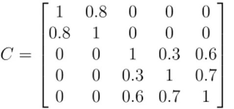
We first generated a design matrixxof sizen = 1000×p= 5 by drawing each observation from a multivariate normal distributionN(µ,Σ). Then, we generated the response according to the logistic regression model (1). We considered as the true parameter values: β = (−0.2,0.5,−0.3,1,0,−0.6), µ = (1,2,3,4,5), and Σ = diag(σ)Cdiag(σ), where σ is the vector of standard deviationsσ = (1,2,3,4,5), andC the correlation matrix
C = 1 0.8 0 0 0 0.8 1 0 0 0 0 0 1 0.3 0.6 0 0 0.3 1 0.7 0 0 0.6 0.7 1 . (6)
Before generating missing values, we performed classical logistic regression on the com-plete dataset, the results (ROC curve) are provided inAppendix A.4. We then randomly in-troduced 10% missing values in the covariates, initially with a missing-completely-at-random (MCAR) mechanism, where each entry has the same probability of being observed.
6.2. The behavior of SAEM
The algorithm was initialized with the parameters obtained after mean imputation, i.e., where missing values of a given variable were replaced by the unconditional mean calculated
τ = 0.6 τ = 0.8 τ= 1.0 0 100 200 300 400 500 0 100 200 300 400 500 0 100 200 300 400 500 0.2 0.4 0.6 0.8 1.0 iteration β1
Figure 1: Convergence plots for β1 obtained with three different values of τ (0.6, 0.8, 1.0). Each color
on the available cases, and then logistic regression was applied to the completed data. For the non-increasing sequence (γk) in the stochastic approximation step of SAEM, we chose γk = 1 during the first k1 iterations in order to converge quickly to a neighborhood of the
MLE, and fromk1iterations on, we setγk= (k−k1)−τ to ensure the almost sure convergence
of SAEM. In order to study the effect of the sequence of stepsizes (γk), we fixed the value of k1 = 50 and used τ = (0.6, 0.8, 1) during the next 450 iterations. Representative plots of
the convergence of SAEM for the coefficientβ1, obtained from four simulated data sets, are
shown in Figure1. For each given simulation, the three sequences of estimates converged to the same solution, but for largerτ, SAEM converged faster and fluctuated less. We therefore use τ = 1 in the following.
6.3. Comparison with other methods
We ran 1000 simulations and compared SAEM to several other existing methods, ini-tially in terms of estimation errors for the parameters. We mainly focused on i) the com-plete case (CC) method, i.e., all rows containing at least one unobserved data value were removed, and ii) multiple imputation by chained equations (mice) with Rubin’s combining
● ● ● ● ● ● ● n = 1000 n = 10000
no NA CC mice SAEM no NA CC mice SAEM
−0.2 0.0 0.2 0.4 Bias of β ^ 3 ● ● ● ● ● ● ● ● ● ● n = 1000 n = 10000
no NA CC mice SAEM no NA CC mice SAEM
0.04 0.08 0.12 Standard error of β ^ 3
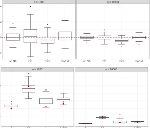
Figure 2: Top: Empirical distribution of the bias of ˆβ3. Bottom: Distribution of the estimated standard
errors of ˆβ3. For each method, the red point corresponds to the empirical standard deviation of ˆβ3calculated
rules [26]. More precisely, missing values are imputed successively by a series of regres-sion models, where each variable with missing data is modeled conditional upon the other variables. For instance, linear regression is used to model continuous variables and binary variables are modeled using logistic regression. More details can be found in van Buuren and Groothuis-Oudshoorn [26]. Finally, we used the dataset without missing values (“no NA”) as a reference, with parameters estimated using the Newton-Raphson algorithm. We varied the number of observations: n= 200,1000,10 000, the missing value mechanism: MCAR or MAR, the percentage of missing values: 10% or 30%, and the correlation structure, either using C given by (6), or an orthogonal design.
Figure2(top) displays the distribution of the estimates ofβ3 forn = 1000 andn = 10 000
under MCAR, with the correlation between covariates given by (6). Simulation results for
n = 200 are presented in the supplementary materials [27]. This plot is representative of the results obtained with the other components of β. As expected, larger samples yielded less variability. Moreover, we observe that in both cases, the estimation obtained by mice
could be biased, whereas SAEM provided unbiased estimates with small variances. Fig-ure 2 (bottom) shows the empirical distribution of the estimated standard error of ˆβ3. For
SAEM it was calculated using the observed Fisher information as described in Section 4.4. With larger n, not only the estimated standard errors–but also variance in the estimation– clearly decreased for all methods. In the case where n = 1000, SAEM and mice slightly overestimated the standard error, while CC underestimated it, on average. Globally, SAEM provided the best results; compared with mice, it gave a similar estimate of the standard error, on average, but with much less variance.
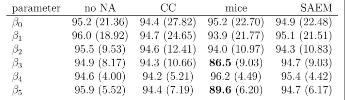
Table 1 shows the coverage probability of the confidence interval for all parameters and inside the parentheses is the average length of the corresponding confidence interval. We would expect coverage of 95%, corresponding to the nominal 95% level. The simulation margin of error for the coverage results is 1.35%. SAEM had between 94.3% and 95.4% coverage, whilemice struggled for certain parameters: the coverage rates for two estimates were 89.6% and 86.5%, significantly below the nominal level. Even though CC showed reasonable results in terms of coverage, the widths of its confidence intervals were still too large. Simulations with smaller sample sizes gave similar results—see supplementary materials [27] for n= 200.
Table 1: Coverage (%) for n= 10 000, correlation C and 10% MCAR, calculated over 1000 simulations.
Bold indicates under-coverage. Inside the parentheses is the average length of corresponding confidence interval over 1000 simulations (multiplied by 100).
parameter no NA CC mice SAEM
β0 95.2 (21.36) 94.4 (27.82) 95.2 (22.70) 94.9 (22.48) β1 96.0 (18.92) 94.7 (24.65) 93.9 (21.77) 95.1 (21.51) β2 95.5 (9.53) 94.6 (12.41) 94.0 (10.97) 94.3 (10.83) β3 94.9 (8.17) 94.3 (10.66) 86.5 (9.03) 94.7 (9.03) β4 94.6 (4.00) 94.2 (5.21) 96.2 (4.49) 95.4 (4.42) β5 95.9 (5.52) 94.4 (7.19) 89.6 (6.20) 94.7 (6.17)
Lastly, Table 2 highlights large differences between the methods in terms of execution time. As an aside, we also implemented the MCEM algorithm [6] using adaptive rejection sampling; even with a very small sample size of n = 200, MCEM took 5 minutes per simu-lation on average. In contrast, multiple imputation took less than 1 second per simusimu-lation, and SAEM less than 10 seconds, which remains reasonable. However, the bias and standard errors for the SAEM and MCEM estimates were quite similar—see supplementary materials [27]. Due to the prohibitive execution time required, for larger sample sizes we did not compare MCEM with the other methods.
Table 2: Comparison of execution times between no NA, MCEM,mice, and SAEM with correlationCand
10% MCAR, forn= 200 andn= 1000, calculated over 1000 simulations.
Execution time (seconds)
for one simulation no NA MCEM mice SAEM
n= 1000 min 2.87×10⁻³ 492 0.64 9.96 mean 4.65×10⁻³ 773 0.70 13.50 max 43.50×10−3 1077 0.76 16.79 n= 200 min 1.26×10⁻³ 67.91 0.24 2.64 mean 2.32×10⁻³ 291.47 0.28 3.91 max 21.53×10−3 1003 0.48 6.04
Results obtained for independent covariates are presented in Figure 3 (right), for esti-mation in the orthogonal design case. SAEM was slightly biased since it estimated non-zero terms for the covariance, but still outperformed CC andmice.
● ● ● ● ● ● ● ● ● ● ●
With correlation Without correlation
no NA CC mice SAEM no NA CC mice SAEM
−0.10 −0.05 0.00 0.05 0.10 Bias of β ^ 3
Figure 3: Empirical distribution of the estimates ofβ3 obtained under MCAR, withn= 10 000 and 10%
6.4. Extended simulations
Missing-at-random mechanisms. We first simulated the pattern of missingness as a binary
vector η = (η1, η2, . . . , ηp) from the Bernoulli distribution, where ηj = 0 indicates that the
corresponding variable xj can be missing whileηj = 1 indicates it is always observed. Then the probability of having missing data in one variable is calculated by a logistic regression model. For example in our case with the realizations of η = (1,0,1,0,0), the probability that covariates (x2, x4, x5) are missing is calculated by a logistic regression model conditional
on x1 and x3. The weights in the linear combination of x1 and x3 have an effect on the
proportion of missingness. We introduced 10% missing values into the covariates using an MAR mechanism. The results presented inAppendix A.5are—as expected—similar to those obtained under MCAR, and show that the parameters are estimated without bias.
Robustness to the normal assumption for covariates. First we generated a design matrix of sizen = 1000×p= 5 by drawing each observation from a multivariate Student distribution
tv(µ,Σ) with v = 5 or v = 20 degrees of freedom, and (µ,Σ) the same as those in the
normal distribution in Section 6.1. Then, we considered the Gaussian mixture model case by generating half of the samples from N(µ1,Σ) and the other half from N(µ2,Σ), where
µ1 = (1,2,3,4,5) and µ2 = (1,1,1,1,1), with the same Σ as previously. Then, we generated
the response according to the same logistic regression model as in Section6.1, and considered either MCAR or MAR mechanisms.
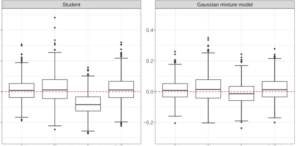
Figure4illustrates the estimation bias of the parameterβ3, andAppendix A.6shows the
coverage for all parameters, with the average length of the corresponding confidence interval in parentheses. This experiment shows that the estimation bias for regression coefficients with the proposed method—even based on normal assumptions—is robust to such model misspecification. Indeed, the bias may increase when covariates do not exactly follow a normal distribution, but the increase is negligible compared to the bias of imputation-based
● ● ● ● ● ● ● ● ● ● ● ● ● ● ● ● ● ● ● ● ● ● ● ● ● ● ● ● ● ● ● ● ● ● ● ● ● ● ● ● ● ● ● ● ● ● ● ● ● ● ● ● ● ● ● ● ● ● ● ● ● ● ● ● ● ● ● ● ● ● ● ● ● ● ● ● ● ● ● ● ● ● ● ● ●
Student Gaussian mixture model
no NA CC mice SAEM no NA CC mice SAEM
−0.2 0.0 0.2 0.4 −0.2 0.0 0.2 0.4 Bias of β ^ 3
Figure 4: Empirical distribution of the bias of ˆβ3 obtained for misspecified models under MCAR, with
methods. We also observe only a small level of under-coverage as compared to mice, and a more reasonable length of confidence interval as compared to CC.
Varying the percentage of missing values. When the percentage of missing values increases, variability in the results increases, but the suggested method still provide satisfactory results—see supplementary materials [27].
Varying the separability of the classes. When the classes are well-separated, SAEM can
exhibit bias and large variance, as illustrated in the supplementary materials [27]. However, logistic regression without missing values also encounters difficulties.
In summary, not only did these simulations show that SAEM leads to estimators with limited bias, but also that we obtained accurate inference by taking into account the addi-tional variance due to missing data.
6.5. Model selection
To look at the performance of the method in terms of model selection, we considered the same simulation scenarios as in Section6.1, with some parameters set to zero. We now describe the results for the case where all parameters in β are zero except β0 =−0.2,β1 =
0.5, β3 = 1, and β5 =−0.6. We compared the BICobs based on the observed log-likelihood,
as described in Section 5, to those based on the complete cases BICcc and obtained from
the the original complete data BICorig.
Table 3 shows, with or without correlation between covariates, the percentage of cases where each criterion selects the true model (C), overfits (O)—i.e., selects more variables than there were, or underfits (U)—i.e., selects less variables than there were. In the case where the variables were correlated, the correlation matrix was the same as in Section 6.1. These results are representative of those obtained in the other simulation settings.
Table 3: For data with or without correlations, the percentage of times that each criterion selects the
correct true model (C), overfits (O), or underfits (U).
Non-Correlated Correlated
Criterion C O U C O U
BICobs 92 3 5 94 2 4
BICorig 96 2 2 93 0 7
BICcc 79 1 20 91 0 9
6.6. Predictions for a test set with missing values
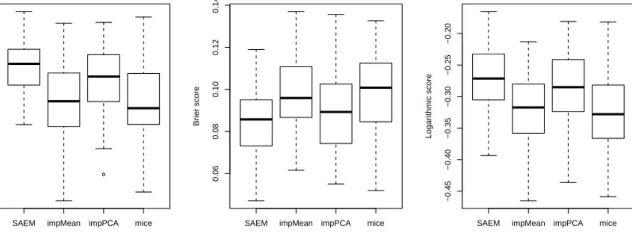
To evaluate the prediction performance on a test set with missing values, we considered the same simulation scenarios for the training set as in Section6.1with sample size 1000×5. We also generated a test set of size 100×5. We compared the approach described in Sec-tion5.3with imputation methods. More precisely, we considered single imputation methods on the training set, followed by classical logistic regression and variable selection by BIC on the imputed dataset. The single imputation methods included i) imputation by the mean
(impMean)ii)imputation by PCA (impPCA) [28], which is based on a low-rank assumption of the data matrix to impute. In addition, we considered multiple imputation using mice. Note that Hentges and Dunsmore [29] showed in a simulation study that imputation meth-ods for MCAR data can perform well when the aim of logistic regression is prediction. For all of the imputation methods, we also imputed the test set independently and then applied the model that had been selected on the training set. Note that this would be a limitation if there was only one individual in the test set, whereas our method does not encounter this issue.
We compared all of these approaches in terms of classical criteria to evaluate the predicted probabilities from the logistic regression. Criteria included AUC (area under the ROC curve), the Brier score [30] and the logarithmic score [31]. Figure 5 shows that on average, marginalizing over the distribution of missing values gave the best performance: the largest AUCs and logarithmic scores, and the smallest Brier scores.
●
SAEM impMean impPCA mice
0.85
0.90
0.95
A
UC
SAEM impMean impPCA mice
0.06 0.08 0.10 0.12 0.14 Br ier score
SAEM impMean impPCA mice
−0.45 −0.40 −0.35 −0.30 −0.25 −0.20 Logar ithmic score
Figure 5: Comparisons of the empirical distribution of the AUC, Brier score, and logarithmic score obtained
on the test set for the proposed SAEM without imputation method, impMean, impPCA, andmice, over 100
simulations.
7. Risk of severe hemorrhage in the TraumaBase context
The fundamental goal of our work is to accelerate and simplify the detection of patients presenting with hemorrhagic shock due to blunt trauma in order to speed up management of this, the most preventable cause of death in major trauma cases. Optimized organization is essential to control blood loss as quickly as possible and reduce mortality.
7.1. Details on the dataset
This study has used data collected from the TraumaBaseR
trauma registry, which collates data from six trauma centers in the Ile-de-France region (Paris area) in France. The centers
progressively joined TraumaBase between January 2011 and June 2015. Since then, data collection has been systematic at these centers. The database is structured in such a way that the algorithm is implemented within it to provide consistency and coherence, with data monitoring performed by a central administrator. Sociodemographic, clinical, biological and therapeutic data (from the pre-hospital phase to discharge, if hospitalized) are systematically recorded for all trauma patients, and all patients transported to the emergency rooms of participating centers are included in the registry. As a result, there were 7495 individuals logged in the trauma data that we investigated, included from January 2011 to March 2016, with ages ranging from 12 to 96. The TraumaBase group decided to focus on patients with blunt trauma so as to be able to compare results with existing prediction rules. Patients with pre-hospital cardiac arrest, penetrating trauma, and missing pre-hospital data, were excluded. This led to 5162 patients being retained in the data set. Based on clinical experience, 16 influential quantitative measurements were included. Detailed descriptions of these and their histograms are shown in Appendix A.7. These variables were chosen because they were all available to the pre-hospital team, and therefore could be used in real situations.
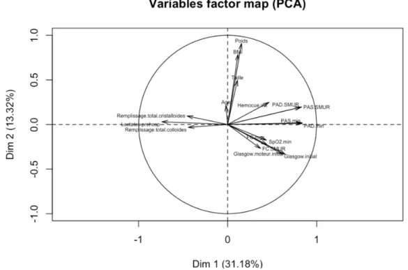
Figure 6: The factor map of the variables from PCA.
There was strong collinearity between variables, as can be seen in the variables’ PCA factor map (obtained by running an EM-PCA algorithm [28] which performs PCA with missing values) in Figure 6, in particular between the minimum systolic (PAS.min) and diastolic blood pressure (PAD.min). Based on expert advice, the recoded variables, SD.min and SD.SMUR (SD.min = PAS.min−PAD.min; SD.SMUR = PAS.SMUR−PAD.SMUR)
were used since they have more clinical significance [32]. Thus, we had 14 variables to predict hemorrhagic shock.
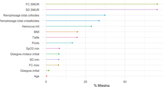
Figure 7: Percentage of missing values in each variable.
Figure7shows the percentage of missingness per variable, varying from 0 to 60%, which demonstrates the importance of taking appropriate account of missing data. Even though there may be many reasons why missingness occurred, overall considering them all to be MAR remains a plausible assumption. For instance, FC.SMUR (heart rate) and SD.SMUR (the pulse pressure measured when the ambulance arrives at the accident site) contain many missing values because doctors collected these data during transportation. However, many other medical institutes and scientific publications use measurements on arrival at the accident scene. Consequently, doctors decided to record these as well, but this occurred after TraumaBase was set up.
We first applied SAEM for logistic regression with all 14 predictors and for the whole dataset. The estimation obtained by SAEM was broadly similar to that obtained by multiple imputation. Next, we used the model selection procedure described in Section5. There were two observations that led to a very small value for the log-likelihood. Upon closer inspection, we found that for patient number 3302, the BMI was obtained using an incorrect calculation, and for patient number 1144, the weight (200 kg) and height (100 cm) values were likely to be incorrect. Hence, the observed log-likelihood also helped us to identify undetected outliers. In the observations’ PCA factor map shown in Figure 8, patient number 3302 (circled in blue) is one of the outliers.
7.2. Predictive performance
We divided the dataset into training and test sets. The training set contained a random selection of 70% of the observations, and the test set contained the remaining 30%. In
Figure 8: The observations’ PCA factor map. Red points are hemorrhagic shock patients, and black points those who did not have hemorrhagic shock. Patient number 3302 (circled in blue) has an incorrectly-calculated BMI.
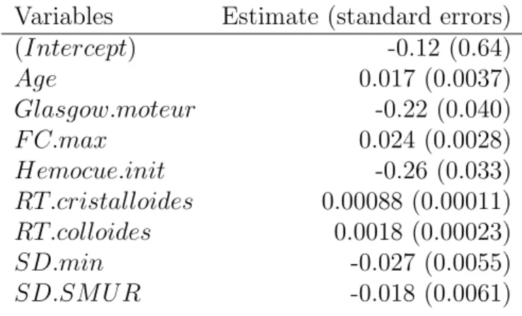
the training set, we selected a model with the approach suggested in Section 5, and used forward selection, resulting in a model with 8 variables. The estimates of parameters and their standard errors are shown in Table4.
Table 4: Estimation ofβ and its standard errors obtained by SAEM, using BIC for model selection.
Variables Estimate (standard errors)
(Intercept) -0.12 (0.64) Age 0.017 (0.0037) Glasgow.moteur -0.22 (0.040) F C.max 0.024 (0.0028) Hemocue.init -0.26 (0.033) RT.cristalloides 0.00088 (0.00011) RT.colloides 0.0018 (0.00023) SD.min -0.027 (0.0055) SD.SM U R -0.018 (0.0061)
The TraumaBase medical team indicated to us that the signs of the coefficients were in agreement with their prior intuition: all things being equal, a) Older people are more likely to have hemorrhagic shock; b) A low Glasgow score implies little or no motor response, which often is the case for hemorrhagic shock patients; c) A typical sign of hemorrhagic
shock is rapid heart rate; d) The more a patient bleeds, the lower their hemoglobin is and more blood must be transfused. It is then more likely they will end up with hemorrhagic shock; e) Therapy involving two types of volume expanders, cristalloides and colloides, can be conducted to treat hemorrhagic shock; f ) If an extremely low pulse pressure is observed, the cause may be a low stroke volume, which is usually the case in hemorrhagic shock.
Next, we assessed the prediction quality on the test set with the usual metrics based on the confusion matrix (false positive rate, false negative rate, etc.). We need to ensure that the cost of a false negative is much more than that of a false positive, as non-recognition of a potential hemorrhagic shock leads to a higher risk of patient mortality. With this in mind, we define the validation error on the test set as:
l(ˆy, y) = 1 n n X i=1 w01{yi=1,yˆi=0}+w11{yi=0,yˆi=1} (7) where w0 and w1 are user defined weight for the cost of a false negative and false positive
respectively, with w0 +w1 = 1. In this way, we can choose a threshold for the logistic
regression by giving values for w0 and w1. For instance, we chose w0w1 = 5, i.e., a false
negative is five times more costly than a false positive. This cost function was chosen after discussions with experts. Note that the test set was also incomplete, so we used the strategy described in Section 5.3 to perform prediction. The confusion matrix of the predictive performance on the test set is shown in Table 5. The associated ROC curve is shown in Figure9, which has an AUC of 0.88.
Observ ed v a lue Predicted outcome 1 0 1 True Positive (102) False Negative (46) 0 False Positive (146) True Negative (1254)
Table 5: Confusion matrix for predictions on the test set.
ROC on validation set − SAEM
False positive rate
T rue positiv e r ate 0.0 0.2 0.4 0.6 0.8 1.0 0.0 0.2 0.4 0.6 0.8 1.0
7.3. Comparison with other approaches
Next, we compared the proposed method to other approaches. Similar to in Section 7.2, we considered single imputation methods followed by classical logistic regression and variable selection on the imputed training dataset, such as single imputation by PCA (impPCA) [28], imputation by Random Forest (missForest) [33], and mean imputation (impMean). We also compared the logistic regression model with other prediction models such as Random Forest (predRF) and SVM (predSVM), both applied on the Random Forest-imputed [33] dataset. We also considered mice: we applied logistic regression with a classical forward selection method, with the BIC calculated on each imputed data set. However, note that there is no straightforward solution for combining multiple imputation and variable selection; we followed the empirical approach suggested in Wood et al. [34] where they select variables that appear in at least half of the models selected in each imputed dataset.
We also considered three rules used by doctors to predict hemorrhagic shock: i)Doctors’ prediction (doctor): the prediction recorded in TraumaBase. This showed whether the doctor considered the patient to be at risk of hemorrhagic shock;ii)The assessment of blood consumption score (ABC): this is an examination usually performed when the patient arrives at the trauma center. As such, the score is not exactly pre-hospital but can be computed very early in a hospitalization; iii) the trauma associated severe hemorrhage score (TASH): this score was also designed for hemorrhage detection, but at a later time-point since it uses some values that are only available after laboratory tests and radiography.
Figure 10 compares the methods in terms of their validation error (7). The splitting of
Figure 10: Empirical distribution of the prediction errors of different methods over 15 random splits of the TraumaBase data.
data (into training and test sets) was repeated 15 times and we fixed the threshold such that the cost of a false negative was five times that of a false positive, i.e., w0w1 = 5. On average, SAEM performed well and with low variability between trials, while all of the imputation methods performed similarly to each other even naive mean imputation. In addition, other prediction methods (Random Forest and SVM) did not give smaller errors on the test sets than the logistic regression models. Lastly, the rules used by doctors, even those using more information than pre-hospital data, did not perform as well as SAEM. Appendix A.8 gives further details on classical criteria (AUC, sensitivity, specificity, accuracy and precision) to compare the predictive performance of the methods. The SAEM approach performed well on average, and particularly well for sensitivity, i.e., it rarely misdiagnosed hemorrhagic shock patients, which gels well with the clinical needs of emergency doctors.
More generally, without defining a specific threshold, we show in Figure 11 the average predictive loss over 15 replicates as a function of the cost ratio{w0
w1 | w0
w1 >1}for all methods.
SAEM had a small error on the test sets given the value of w0w1, especially when we increased the cost of false negatives. Note that the errors for the doctors’ rules and ABC increased as a function of the cost importance w0w1, which means that these rules are more conservative than SAEM is, which may be problematic in this setting. Also, missForest had excellent predictive capabilities which is consistent with the results of Josse et al. [35]. However, it is difficult to interpret the results from random forest in terms of selected variables, which is often crucial for emergency doctors.
Figure 11: Average prediction errors of different methods as a function of the cost ratio{w0
w1 |
w0
w1 >1}taken over 15 random splits of the TraumaBase data.
Note that even if our proposed methodology is based on the assumption of normally distributed covariates, its performance is better than the predictions made by widely-used medical criterion in terms of prediction error. Further discussion on the normal assumption is provided inAppendix A.7. In addition, it should be noted that the proposed methodology can be extended to other assumptions about the joint distribution of covariates, such as a mixture of distributions.
In summary, based on the TraumaBase application and comparisons with other methods, we have demonstrated that this new approach has the ability to outperform existing popular methods that deal with missing data.
8. Discussion
In this paper, we have developed a comprehensive joint-modeling framework for logistic regression with missing values. The method is implemented in the R package misaem. The experiments we have performed indicate that this method is computationally efficient and easy to implement. In addition, compared with multiple imputation—especially in the case of correlation between variables—estimation using SAEM is less biased than other methods and generally leads to interval-estimate coverage that is close to the nominal level. Based on our algorithm, model selection with BIC and missing data can be performed in a natural way. In view of the results reported in this article, we have been invited by emergency-room doctors in one of the TraumaBase centers to implement the missing-data methodology outlined here in a prospective study to evaluate its performance in a real-time clinical setting. Paths for possible future research include further developing the method to handle both quantitative and categorical data. This paper focused on making inference with missing values, but we have also suggested a method to predict from a test set with missing val-ues. More work could be done in the direction of supervised learning with missing values, especially when we want to better estimate the variance of predictions. Extensions of the methods of Schafer and Schenker [36] could be considered. In addition, in the TraumaBase dataset, it would be reasonable to expect to have both MAR and missing-not-at-random (MNAR) values. MNAR means that missingness is related to the missing values themselves, and therefore a more correct methodology would require incorporating models for missing data mechanisms. As a final note, our proposed method may be quite useful in a causal inference framework, especially for propensity score analysis, which estimates the effect of a treatment, policy, or other intervention. Indeed, inverse probability weighting methods (IPW) are often performed with logistic regression, and the proposed method offers a po-tential solution for times where there are missing values in the covariates.
Appendix A. Appendix
Appendix A.1. Missingness mechanisms
Missing-completely-at-random (MCAR) means that there is no relationship between the missingness of the data and any values, observed or missing. In other words, MCAR means:
p(Mi|y, xi, φ) = p(Mi|φ).
Missing-at-random (MAR) means that the probability to have missing values may depend on the observed data, but not on the missing data. We must carefully define what this means in our case by decomposing the data xi into a subset x
(mis)
i of data that “can be missing”,
and a subset x(obs)i of data that “cannot be missing”, i.e,. that is always observed. Then, the observed data xi,obs necessarily includes the data that can be observed x
(obs)
i , while the
data that can be missingx(mis)i includes the missing dataxi,mis. Thus, the MAR assumption
implies that, for each individual i,
p(Mi|yi, xi;φ) = p(Mi|yi, x
(obs)
i ;φ)
=p(Mi|yi, xi,obs;φ).
The MAR assumption implies that the observed likelihood can be maximized and the dis-tribution of M can be ignored [4]. Indeed,
L(θ, φ;y, xobs, M) =p(y, xobs, M;θ, φ) = n Y i=1 p(yi, xi,obs, Mi;θ, φ) = n Y i=1 Z p(yi, xi, Mi;θ, φ)dxi,mis = n Y i=1 Z p(yi, xi;θ)p(Mi|yi, xi;φ)dxi,mis = n Y i=1 Z p(yi, xi;θ)p(Mi|yi, xi,obs;φ)dxi,mis = n Y i=1
p(Mi|yi, xi,obs;φ)×
n
Y
i=1
Z
p(yi, xi;θ)dxi,mis
=p(M|y, xobs;φ)×p(y, xobs;θ)
=p(M|y, x(obs);φ)×p(y, xobs;θ).
Therefore, to estimate θ, we aim to maximizeL(θ;y, xobs) = p(y, xobs;θ). Appendix A.2. Metropolis-Hastings sampling
During SAEM iterations, Metropolis-Hastings sampling is performed as in Algorithm1, with target distributionf(xi,mis) =p(xi,mis|xi,obs, yi;θ) and proposal distributiong(xi,mis) =
Algorithm 1Metropolis-Hastings sampling.
Input: An initial sample x(0)i,mis ∼g(xi,mis);
for s= 1,2, . . . , S do
Generate x(i,smis) ∼g(xi,mis);
Generate u∼ U[0,1]; Calculate the ratio w= f(x
(s) i,mis)/g(x (s) i,mis) f(x(i,smis−1))/g(x(i,smis−1)); if u < w then Accept x(i,smis) ; else x(i,smis) ←x(i,smis−1); end if end for Output: (x(i,smis) ,1≤i≤n,1≤s ≤S).
Appendix A.3. Calculation of the observed information matrix
Procedure 2shows how we calculate the observed information matrix.
Procedure 2Calculation of the observed information matrix.
Input: After drawing MH samples (x(i,smis) ,1 ≤ i ≤ n,1 ≤ s ≤ S) for unobserved data (xi,mis,1 ≤ i ≤ n), we have imputed observations, noted as (z
(s)
i ,1 ≤ i ≤ n,1 ≤ s ≤ S),
where zij(s)=xi,obs, if xij is observed; else z
(s) ij =x (s) i,mis. for n= 1,2, . . . , n do for s= 1,2, . . . , S do
Calculate the gradient: ∇fis = ∂LL(θ;xi,obs,x (s) i,mis,yi) ∂β =z (s) i yi− exp( ˆβ0+Pp j=1βˆjz (s) ij ) 1+exp( ˆβ0+Pp j=1βˆjz (s) ij ) ; Calculate the Hessian matrix:
His = ∂2LL(θ;x i,obs,x (s) i,mis,yi) ∂β∂βT =−z (s) i z (s) i T exp( ˆβ0+Pp j=1βˆjz (s) ij ) 1+exp( ˆβ0+Pp j=1βˆjz(ijs)) 2; ∆i ← 1s[(s−1)∆i+∇fis]; Di ← 1s[(s−1)Di+His]; Gi ← 1s[(s−1)Gi+∇fis∇fisT]; end for ˆ IS( ˆβ)←IˆS( ˆβ)−(Di+Gi−∆i∆Ti ); end for Output: IˆS( ˆβ).
Appendix A.4. Logistic regression on a simulated complete dataset
FigureA.12 shows the ROC curve on a simulated complete dataset. The corresponding AUC (for the training set) is 0.8976.
Appendix A.5. Simulation results for missing-at-random data
We consider a missing-at-random mechanism to generate data. Figure A.13shows that the biases were very similar to those obtained under a MCAR mechanism, and parameters were estimated without bias.
ROC on the original dataset
False positive rate
Tr ue positiv e r ate 0.0 0.2 0.4 0.6 0.8 1.0 0.0 0.2 0.4 0.6 0.8 1.0
Figure A.12: ROC curve on a simulated complete dataset.
Figure A.13: Empirical distribution of the bias of ˆβ3
obtained under an MAR mechanism, with n= 1000
and 10% missing values.
Appendix A.6. Simulation results for model misspecification: coverage
Table A.6 shows the coverage for all parameters, and the average lengths of the corre-sponding confidence intervals in parentheses.
Table A.6: Coverage (%) forn= 1000, MCAR, and misspecified models, calculated over 1000 simulations.
Bold indicates under-coverage. Inside the parentheses is the average length of the corresponding confidence interval over 1000 simulations (multiplied by 100).
parameter no NA CC mice SAEM
Student distribution: (v = 5) β0 94.7 (68.02) 94.3 (84.14) 94.6 (67.69) 93.8 (68.25) β1 95.2 (54.78) 94.2 (72.15) 91.7 (61.96) 93.5 (63.05) β2 94.9 (27.66) 94.6 (36.39) 91.4 (31.21) 93.7 (31.84) β3 94.9 (26.76) 94.3 (35.24) 81.5 (30.46) 94.7 (29.98) β4 95.2 (11.52) 95.4 (15.16) 95.8 (12.94) 95.5 (12.88) β5 93.7 (17.63) 94.9 (23.22) 83.4 (20.40) 93.3 (19.93) Gaussian mixture: β0 94.8 (57.54) 95.2 (75.42) 95.4 (61.95) 95.0 (61.33) β1 94.7 (58.00) 96.2 (76.05) 95.4 (66.66) 95.3 (66.13) β2 94.3 (28.49) 95.3 (37.35) 95.3 (32.65) 94.0 (32.50) β3 94.7 (26.16) 94.9 (34.38) 94.9 (28.91) 94.5 (29.10) β4 94.4 (12.68) 94.4 (16.60) 94.4 (14.24) 94.7 (14.09) β5 95.3 (17.70) 94.7 (23.25) 94.7 (19.86) 95.3 (19.92)
Appendix A.7. Definitions of variables in the TraumaBase dataset
In this section, we define the selected quantitative variables: • Age: Age.
• P oids: Weight. • T aille: Height.
• BM I: Body Mass index, BM I = (W eightHeightininmkg)2
• Glasgow: Glasgow Coma Scale.
• Glasgow.moteur: Glasgow Coma Scale motor component.
• P AS.min: The minimum systolic blood pressure.
• P AD.min: The minimum diastolic blood pressure.
• F C.max: The maximum number of heart beats per unit time (usually a minute).
• P AS.SM U R: Systolic blood pressure at ambulance arrival. • P AD.SM U R: Diastolic blood pressure at ambulance arrival. • F C.SM U R: Heart rate at ambulance arrival.
• Hemocue.init: Capillary hemoglobin concentration.
• SpO2.min: Oxygen saturation.
• Remplissage.total.colloides (or RT.colloides): Fluid expansion colloids.
• Remplissage.total.cristalloides (or RT.cristalloides): Fluid expansion cristalloids.
• SD.min(= P AS.min−P AD.min): Pulse pressure for the minimum values of diastolic
and systolic blood pressure.
• SD.SM U R(= P AS.SM U R−P AD.SM U R): Pulse pressure at ambulance arrival.
Figure A.14 shows the histogram and the empirical cumulative distribution function of some of the covariates in TraumaBase. Several of these are not symmetric. In practice, it is possible to consider that suitable transformation of covariates can be approximated by normal distributions. For example, transformations of the form log(c+x) and log(c−x), may be appropriate for right-skewed and left-skewed distributions respectively. We applied the proposed methodology to the real dataset after the log-transformation. However, the prediction results from cross-validation did not show any advantage to transforming the variables. Indeed when a log transformation is used as a prepossessing step, it only operates on the observed part, which is appropriate under MCAR values. Consequently, we have decided not to use any transformation on the dataset.
SD.min SD.SMUR SpO2.min
FC.SMUR Hemocue.init Poids
Age BMI FC.max
0 100 −100 0 100 0 25 50 75 100 50 100 150 200 0 5 10 15 20 50 100 150 200 25 50 75 100 25 50 75 0 50 100 150 200 0.000 0.005 0.010 0.015 0.020 0.00 0.01 0.02 0.03 0.00 0.05 0.10 0.15 0.00 0.03 0.06 0.09 0.12 0.0 0.1 0.2 0.3 0.4 0.00 0.01 0.02 0.03 0.00 0.01 0.02 0.03 0.00 0.01 0.02 0.00 0.01 0.02 0.03 value density
(a) Histograms of covariates
SD.min SD.SMUR SpO2.min
FC.SMUR Hemocue.init Poids
Age BMI FC.max
−8 −4 0 4 8 −5 0 5 −15 −10 −5 0 −2 0 2 4 −7.5 −5.0 −2.5 0.0 2.5 0 5 −2 0 2 0 5 10 15 −4 −2 0 2 4 6 0.00 0.25 0.50 0.75 1.00 0.00 0.25 0.50 0.75 1.00 0.00 0.25 0.50 0.75 1.00 0.00 0.25 0.50 0.75 1.00 0.00 0.25 0.50 0.75 1.00 0.00 0.25 0.50 0.75 1.00 0.00 0.25 0.50 0.75 1.00 0.00 0.25 0.50 0.75 1.00 0.00 0.25 0.50 0.75 1.00 value y
(b) Empirical cumulative distributions Figure A.14: Empirical distributions of variables from TraumaBase. (a) Histograms of covariates; (b) The black line is the empirical cumulative distribution while the red one corresponds to the normal distribution.
Appendix A.8. Details on the predictive performance on TraumaBase data
Details on the predictive performance on TraumaBase data are given in Table A.7.
Table A.7: Comparisons of the mean of the predictive performance (values are multiplied by 100) of
different methods that can deal with missing data. AUC is the area under the ROC curve; the accuracy is the number of true positives plus true negatives, divided by the total number of observations; the sensitivity is the true positive rate; the specificity is the true negative rate; the precision is the number of true positives over all positive predictions. Best results are shown in bold.
Metrics SAEM missForest impMean impPCA mice predRF predSVM
AUC 88.5 88.8 88.9 89.0 87.7 88.0 80.4 Accuracy 86.9 87.0 87.3 86.7 85.3 87.2 88.3 Precision 41.1 41.6 42.2 41.0 37.9 41.6 44.0 Sensitivity 74.6 74.3 73.2 75.0 75.2 71.5 66.0 Specificity 88.2 88.4 88.8 87.9 86.4 88.9 90.6 Supplementary material
R-package: The R packagemisaem containing the implementation of the SAEM algorithm to fit the logistic regression model with missing data is available on CRAN [20].
Additional supplementary materials: Additional simulation results can be found here: [27].
Acknowledgment
Wei Jiang was supported by grants from Region Ile-de-France: https://www.dim-mathinnov. fr. The authors are thankful for fruitful discussion with Kevin Bleakley and Antoine Ogier.
References
[1] A. P. Dempster, N. M. Laird, D. B. Rubin, Maximum likelihood from incomplete data via the EM algorithm, Journal of the Royal Statistical Society. Series B (Methodological) 39 (1977) 1–38.
[2] X.-L. Meng, D. B. Rubin, Using EM to obtain asymptotic variance-covariance matrices: The SEM algorithm, Journal of the American Statistical Association 86 (1991) 899–909.
[3] T. A. Louis, Finding the observed information matrix when using the EM algorithm, Journal of the Royal Statistical Society. Series B (Methodological) 44 (1982) 226–233.
[4] R. J. Little, D. B. Rubin, Statistical Analysis with Missing Data, second ed., John Wiley & Sons, Inc., 2002.
[5] S. Seaman, J. Galati, D. Jackson, J. Carlin, What is meant by “missing at random”?, Statist. Sci. 28 (2013) 257–268.
[6] J. G. Ibrahim, M.-H. Chen, S. R. Lipsitz, Monte Carlo EM for missing covariates in parametric
regression models, BIOMETRICS 55 (1999) 591–596.
[7] J. G. Ibrahim, M.-H. Chen, S. R. Lipsitz, A. H. Herring, Missing-data methods for generalized linear models: A comparative review, Journal of the American Statistical Association 100 (2005) 332–346. [8] G. C. G. Wei, M. A. Tanner, A Monte Carlo implementation of the EM algorithm and the poor man’s
data augmentation algorithms, Journal of the American Statistical Association 85 (1990) 699–704. [9] G. McLachlan, T. Krishnan, The EM algorithm and extensions, Wiley series in probability and
statis-tics, 2. ed ed., Wiley, Hoboken, NJ, 2008.
[10] W. R. Gilks, P. P. Wild, Adaptive rejection sampling for Gibbs sampling, Appl. Statist 41 (1992) 337–348.
[11] M. Lavielle, Mixed Effects Models for the Population Approach: Models, Tasks, Methods and Tools, Chapman and Hall/CRC, 2014.
[12] G. Claeskens, F. Consentino, Variable selection with incomplete covariate data, Biometrics 64 (2008) 1062–9.
[13] F. Consentino, G. Claeskens, Missing covariates in logistic regression, estimation and distribution selection, Statistical Modelling 11 (2011) 159–183.
[14] J. Jiang, T. Nguyen, J. S. Rao, The E-MS algorithm: Model selection with incomplete data, Journal of the American Statistical Association 110 (2015) 1136–1147.
[15] Y. Liu, Y. Wang, Y. Feng, M. M. Wall, Variable selection and prediction with incomplete
high-dimensional data, Ann. Appl. Stat. 10 (2016) 418–450.
[16] W. K. Chow, A look at various estimators in logistic models in the presence of missing values, Technical Report, RAND CORP SANTA MONICA CA, 1979.
[17] K. Yuen Fung, B. A. Wrobel, The treatment of missing values in logistic regression, Biometrical Journal 31 (1989) 35 – 47.
[18] D. B. Rubin, Multiple Imputation for Nonresponse in Surveys, volume 307, John Wiley & Sons, 2009. [19] R Core Team, R: A Language and Environment for Statistical Computing, R Foundation for Statistical
Computing, Vienna, Austria, 2017.
[20] W. Jiang, misaem: Logistic regression with missing covariates, 2019. R package version 0.9.1.
[21] W. Jiang, Codes and implementations for ”Logistic regression with missing covariates – parameter
estimation, model selection and prediction within a joint-modeling framework”,https://github.com/
[22] S. I. Hay, et al., Global, regional, and national disability-adjusted life-years (dalys) for 333 diseases and injuries and healthy life expectancy (hale) for 195 countries and territories, 1990–2016: a systematic analysis for the global burden of disease study 2016, The Lancet 390 (2017) 1260 – 1344.
[23] S. R. Hamada, T. Gauss, F.-X. Duchateau, J. Truchot, A. Harrois, M. Raux, J. Duranteau, J. Mantz, C. Paugam-Burtz, Evaluation of the performance of french physician-staffed emergency medical service in the triage of major trauma patients, Journal of Trauma and Acute Care Surgery 76 (2014) 1476–1483.
[24] S. R. Hamada, T. Gauss, J. Pann, M. W. D¨unser, M. L´eone, J. Duranteau, European trauma guideline
compliance assessment: The ETRAUSS study, Critical care 19 (2015) 423.
[25] B. Delyon, M. Lavielle, E. Moulines, Convergence of a stochastic approximation version of the EM algorithm, The Annals of Statistics 27 (1999) 94–128.
[26] S. van Buuren, K. Groothuis-Oudshoorn, mice: Multivariate imputation by chained equations in R, Journal of Statistical Software 45 (2011) 1–67.
[27] W. Jiang, Additional supplementary materials for ”Logistic regression with missing covariates –
parameter estimation, model selection and prediction within a joint-modeling framework”, https:
//github.com/wjiang94/miSAEM_logReg/tree/master/Supplement, 2019.
[28] J. Josse, F. Husson, missMDA: A package for handling missing values in multivariate data analysis, Journal of Statistical Software 70 (2016) 1–31.
[29] A. L. Hentges, I. R. Dunsmore, Predictive distributions in binary models with missing data, Commu-nications in Statistics-Simulation and Computation 27 (1998) 735–759.
[30] G. W. Brier, Verification of forecasts expressed in terms of probability, Monthly Weather Review 78 (1950) 1–3.
[31] I. J. Good, Rational decisions, Journal of the Royal Statistical Society. Series B (Methodological) (1952) 107–114.
[32] S. R. Hamada, A. Rosa, T. Gauss, J.-P. Desclefs, M. Raux, A. Harrois, A. Follin, F. Cook, M. Bou-tonnet, A. Attias, S. Ausset, G. Dhonneur, O. Langeron, C. Paugam-Burtz, R. Pirracchio, B. Riou,
G. de St Maurice, B. Vigu´e, A. Rouquette, J. Duranteau, Development and validation of a pre-hospital
“Red Flag” alert for activation of intra-hospital haemorrhage control response in blunt trauma, Critical Care 22 (2018) 113.
[33] D. J. Stekhoven, P. Buehlmann, MissForest – non-parametric missing value imputation for mixed-type data, Bioinformatics 28 (2012) 112–118.
[34] A. M. Wood, I. R. White, P. Royston, How should variable selection be performed with multiply imputed data?, Statistics in Medicine 27 (2008) 3227–3246.
[35] J. Josse, N. Prost, E. Scornet, G. Varoquaux, On the consistency of supervised learning with missing values, arXiv e-prints (2019). ArXiv:1902.06931.
[36] J. L. Schafer, N. Schenker, Inference with imputed conditional means, Journal of the American