Alternating model trees

(1)

Alternating Model Trees

Eibe Frank

Department of Computer Science

University of Waikato Hamilton, New Zealand

Michael Mayo

Department of Computer

Science University of Waikato Hamilton, New Zealand

Stefan Kramer

Institute of Computer Science

University of Mainz Mainz, Germany

ABSTRACT

Model tree induction is a popular method for tackling re-gression problems requiring interpretable models. Model trees are decision trees with multiple linear regression mod-els at the leaf nodes. In this paper, we propose a method for growing alternating model trees, a form of option tree for regression problems. The motivation is that alternating decision trees achieve high accuracy in classification prob-lems because they represent an ensemble classifier as a single tree structure. As in alternating decision trees for classifi-cation, our alternating model trees for regression contain splitter and prediction nodes, but we use simple linear re-gression functions as opposed to constant predictors at the prediction nodes. Moreover, additive regression using for-ward stagewise modeling is applied to grow the tree rather than a boosting algorithm. The size of the tree is determined using cross-validation. Our empirical results show that alter-nating model trees achieve significantly lower squared error than standard model trees on several regression datasets.

Categories and Subject Descriptors

I.2.6 [Artificial Intelligence]: Learning

General Terms

Algorithms, Experimentation, Performance

Keywords

Regression, alternating model trees

1. INTRODUCTION

Alternating decision trees [5] provide the predictive power of decision tree ensembles in a single tree structure. They are a variant of option trees [3, 9], i.e., decision trees augmented with option nodes, and grown using boosting. Existing ap-proaches for growing alternating decision trees focus on clas-sification problems. In this paper, we investigate alternating

Permission to make digital or hard copies of all or part of this work for personal or classroom use is granted without fee provided that copies are not made or distributed for profit or commercial advantage and that copies bear this notice and the full citation on the first page. To copy otherwise, to republish, to post on servers or to redistribute to lists, requires prior specific permission and/or a fee.

SAC’15April 13-17, 2015, Salamanca, Spain.

model trees for regression, inspired by work on model trees for regression [15] and work on growing alternating decision trees for multi-class classification [8].

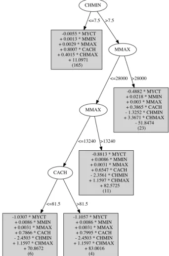
Model trees for regression are decision trees with linear regression models at the leaf nodes. They were originally proposed by Quinlan [15]. An open-source implementation, called M50, was presented in [18] and has proven to be suc-cessful in many practical applications, e.g., [16, 2, 14, 4, 13, 17]. An example model tree grown using M50 is shown in Figure 1. The inclusion of linear regression models rather than constant predictors at the leaf nodes is essential: stan-dard regression trees with constant predictors produce much less accurate predictions than model trees [15].

M5 trees are grown using the standard top-down approach for growing decision trees. Once an unpruned tree has been grown, multiple linear regression models are placed at each node of the tree. Following this, the tree is pruned, poten-tially replacing large subtrees by a single linear regression model. Finally, the linear regression models along the path from the root node of the tree to each leaf node are combined into a single linear regression model at the leaf node using a “smoothing” process that produces a linear combination of linear regression models. For further details, see [15, 18].

The learning algorithm for alternating model trees we present in this paper grows trees using additive regression. In [8], alternating decision trees for multi-class classification are grown using additive logistic regression, a statistical vari-ant of boosting. The process we apply in this paper is very similar, applying forward stagewise additive modeling for minimization of squared error rather than maximization of multinomial likelihood. The key difference of our method is that we use (simple) linear regression models instead of con-stant predictors in the tree so that we can obtain competitive predictive performance on regression problems. Moreover, to reduce computational complexity and data fragmenta-tion, splits on numeric attributes at splitter nodes are re-stricted to the median value of each attribute rather than arbitrary points identified by a split selection criterion.

2. ALTERNATING MODEL TREES

We assume that we have a training datasetD withn in-stances consisting of m valued attributes and a real-valued target attribute. The learning algorithm is provided withninstances (x~i, yi), with 1≤i≤n, wherex~iis a vector of attribute values andyiis the associated target value. The task is to learn a model such that, given a new~x, this model can be used to predict the corresponding value y. In this paper, we assume that the goal is to minimize the squared

(2)

��

Figure 1: M50 model tree for machine-cpu data

error of the model between the predicted and actual target values. Furthermore, we assume that the data is indepen-dently and identically distributed.

2.1 Forward Stagewise Additive Modeling

Our method for learning additive model trees applies the basic algorithm for additive regression using forward stage-wise additive modeling [6]. The strategy is to iteratively correct the predictions of an additive modelFj(~x) by taking the residual errors it makes on the training data—the differ-ences between the actual and predicted target values—and applying a base learner that learns to predict those residuals. The modelfj+1(~x) output by the base learner is then

ap-pended to the additive model and the residuals are updated for the next iteration.

More precisely, we fit a model consisting ofkbase models, Fk(~x) =

k

X

j=1

fj(~x) (1)

in a forward stagewise manner so that the squared error n

X

i=1

(Fk(~xi)−yi)2 (2) over thentraining examples (~xi, yi) is minimized.

Input:D: training data,BL: base learner,I: number of iterations to perform,λ: shrinkage parameter ∈(0,1]

Output: L: list containing ensemble predictor

L:= empty list L.add(1 n P (~x,y)∈Dy) foreach(~x, y)∈Ddo (~x, y) := (~x, y−L.f irst().prediction(~x)) end while|L| ≤Ido

L.add(BL.buildM odel(D))

foreach(~x, y)∈Ddo

(~x, y) := (~x, y−λ×L.last().prediction(~x))

end end returnL

Algorithm 1:Additive regression using forward stagewise additive modeling

In a particular iterationk, we fit a base modelfk(~x) (e.g., a regression stump) to the residualsy−Fk−1(~x) remaining

from the k−1 previous iterations. We fit these residuals by minimizing the squared error between them and the base model’s predictionsfk(~x).

In this manner, we ensure that the squared error of the additive model is minimized, assuming the existing part of the modelFk−1(~x) can no longer be modified:

n X i=1 ((yi−Fk−1(~xi))−fk(~xi))2 = n X i=1 (yi−(Fk−1(~xi) +fk(~xi)))2= n X i=1 (yi−Fk(~xi))2

This is thus a greedy algorithm to fit an additive regression model by minimizing squared error.

Pseudo code for the algorithm is shown in Algorithm 1. It has three arguments: the base regression learner to use, the number of iterations to perform, and the value of the shrinkage parameter used to control overfitting. The algo-rithm first calculates the mean target value and makes this predictor the first element of the additive model. Subtract-ing the mean establishes the initial set of residuals. In each iteration of additive regression, the base regression scheme is applied to learn to predict the residuals. Subsequently, the predicted residuals are subtracted from the actual residuals to establish the new set of residuals for the next iteration. This is repeated for the given number of iterations.

The shrinkage parameter is a value in (0,1]. (A value of 1 means that no shrinkage is performed.) In the algo-rithm, the predictions of the base learner are multiplied by the shrinkage value when the residuals are calculated. When the shrinkage value is reduced by the user, the predictions of each base model are dampened before being included in the additive model. Because the mean predictor is the first element in the model, and is not affected by the shrinkage parameter, the predictions of the additive model are there-fore shrunk towards the mean. This makes it possible to perform regularization of the model.

The prediction step is shown in Algorithm 2. It is straight-forward: the predictions of all base models are simply mul-tiplied by the shrinkage value and added to the mean target value from the training data. This is then the final predic-tion of the additive model.

(3)

Input:~x: the instance to make a prediction for,L: list of regressors

Output:y: the prediction

y=L.f irst().prediction(~x) foreachM∈Ldo if M6=L.f irst()then y=y+λ×M.prediction(~x) end end returny

Algorithm 2:Generating a prediction using the additive regression model ��

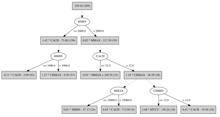
Figure 2: Alternating decision tree with five splitter nodes grown from pima-indians diabetes data

2.2 Constructing Alternating Model Trees

An alternating decision tree consists of two types of nodes: splitter nodes and prediction nodes [5]. In the classification case, it is grown by adding one splitter node and two predic-tion nodes in each iterapredic-tion of the boosting algorithm that generates the tree. A splitter node is the same as an internal node in a standard decision tree and divides the data based on a chosen attribute-value test. Prediction nodes contain numeric scores that are used to make a prediction. When an instance is to be classified, it is routed down all applicable paths in the tree and the numeric scores of all visited pre-diction nodes are summed to yield the final prepre-diction. For example, in the two-class classification case, the sum may be positive, in which case the positive class is predicted; otherwise, the negative class is predicted.

Figure 2 shows an alternating decision tree grown using the algorithm from [5], for the two-class pima-indians dia-betes data available from the UCI repository of datasets [1]. Five boosting iterations where performed to grow this tree so that five splitter nodes are included. The root node has three prediction nodes attached to it. When a prediction is to be made, all three options need to be considered.

Consider an instance that has the following values for the attributes used in the tree: plas = 130, mass = 27.1 and age= 30. The score for this instance involves five prediction nodes and would be−0.311 + 0.541 + 0.148 + 0.226−0.302 = 0.302 >0. Hence, tested positive would be the class pre-dicted for this instance.

An alternating decision tree is an option tree because each

prediction node can have multiple splitter nodes as succes-sors (or none, in which case it is a leaf node). In each boost-ing iteration, a prediction node in the current version of the alternating tree is identified, and a splitter node, with two new prediction nodes attached to it, is added to it as a suc-cessor. The particular prediction node chosen for this and the split applied at the splitter node are selected such that the loss function of the boosting algorithm is minimized.

We can view an alternating decision tree as a collection of if-then rules, where each path in the tree corresponds to a rule. In each iteration of the boosting algorithm, a particular rule is chosen for extension by an additional attribute-value test (implemented by the splitter node), and two extended versions of the rule are added to the rule set. Thus, we can view the process of growing an alternating decision tree as an application of boosting with a base learner that grows restricted if-then rules: the two new rules added in a par-ticular iteration consist of a prefix that already exists in the tree, one new test is added to both rules, and the new rules include appropriately chosen values on the right-hand side.

We can easily adapt this method for growing an alternat-ing decision tree so that it can be applied to regression prob-lems. Given the algorithm for generating an additive model for regression discussed above, we can grow an alternating decision tree for regression by applying an appropriate base learner. In each iteration of additive regression, we add one splitter node and two prediction nodes to the tree. The pa-rameters of these nodes and their location in the alternating tree are chosen so that squared error is minimized.

However, because we want to grow alternating model trees, we do not simply add constant values at the prediction nodes, but rather apply simple linear regression functions.1 A splitter node is constructed by considering splits on all available attributes in the data, splitting on the median at-tribute value for the corresponding data that reaches the node to be split, and fitting two simple linear regression models to the subsets created by the split. The two at-tributes for the simple linear regression models are chosen so that squared error is minimized.

Of all available splits, one for each attribute and existing prediction node, the split that minimizes the squared error of the alternating tree is chosen, and the corresponding two linear regression models are placed at the two new prediction nodes that are attached to the new splitter node. Note that the two simple linear regression models for the two subsets of data generated by the median-based split can be based on different attributes. For each subset, all attributes are considered, and that particular attribute is chosen whose simple linear regression model minimizes squared error.

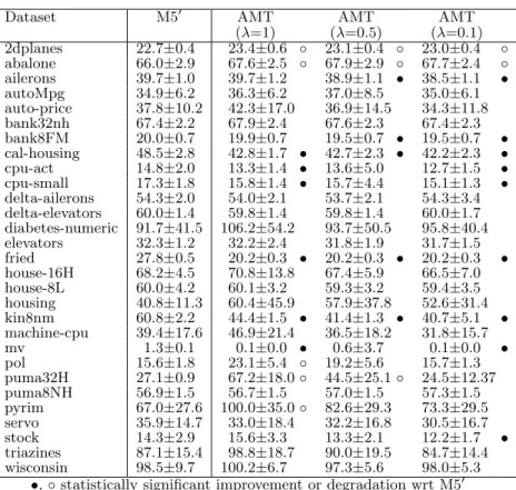
Figure 3 shows an example model tree for the machine-cpu data. Five iterations of additive regression where performed so the tree contains five splitter nodes and 11 prediction nodes, including the root node which simply predicts the mean target value from the training data. The lowest level of the tree has two splitter nodes that are attached to the same prediction node. Hence, if an instance reaches this prediction node, both successors need to be visited and a prediction obtained from both of them. The numbers in

1

In contrast to amultiplelinear regression model as used in M5, a simplelinear regression model is a regression model based on a single, appropriately chosen, predictor attribute. Simple linear regression models are also used in the model tree inducers presented in [10, 11].

(4)

��

Figure 3: Alternating model tree for machine-cpu data

brackets show the number of training instances that reach a particular prediction node. With continuous data, they are equal for the two successors of a prediction node, because the median value is used for splitting, but this data has discrete values and hence the splits are not balanced.

Algorithm 3 has the pseudo code for growing the alternat-ing model tree. It employs three types of objects:

• SplitterN odeobjects that contain a reference to their parent prediction node; the score—reduction in squared error—they achieve; the parameters for the split (at-tribute index and value of split point); and references to the two successor prediction nodes.

• P redictionN odeobjects that contain a reference to the regression model employed; the data associated with the node; and a list of successors, holding references to splitter nodes that are its successors.

• SLRobjects that perform simple linear regression based on the data for a given attribute and the target; they also contain the sum of squared errors (SSE) achieved and are able to yield a prediction for a new instance. The algorithm maintains a list of prediction nodes that initially only contains the predictor of the mean. The target values are also centered, just as in Algorithm 1. Then, a given user-specified number of iterations is performed, and in each iteration, a newSplitterN odeis added to a selected prediction node. To select this node, the algorithm iter-ates through allP redictionN odeobjects already in the list. For each prediction node, the current sum of squared er-rors (i.e. sum of squared residuals/target values) associated

with the data pertaining to this node is established first, so that the reduction of squared error that is achieved by a split attached to this node can be computed later. Then, all attributes are evaluated for a median-based split: for each split, the data is divided into two subsets and the best linear model (lowest SSE) is found for each subset. If the current split yields a larger reduction in SSE than the previous best one, the information for the splitter node is updated.

Once the best SplitterN ode has been constructed, it is attached to its parent node, and its two attached prediction nodes are added to the global list of prediction nodes so that they become available for selection in the next iteration of the algorithm. After this, the residuals/target values are up-dated for the two subsets of data associated with the split. Note that we assume that only one copy of each instance (~x, y) inD is maintained in memory, and that this copy is modified when the residuals are updated, i.e., we use mu-table tuples. Hence, the effect of the update is global and affects the data to be considered in the next iteration atall

applicable prediction nodes in the tree. Hence, the process is consistent with the algorithm for additive regression.

Algorithm 4 shows the pseudo code for making predic-tions using the tree. It is given the root node of the tree and maintains a queue of prediction nodes to include in the prediction. The root node is the first element in the queue. As it predicts the mean target value from the training data, no shrinkage is applied to its prediction. If the queue is not empty, the first prediction node is popped off the queue and its prediction is added to the running sum. Then, all split-ter nodes that are successors of the current prediction node are evaluated, and the appropriate successor of each splitter

(5)

Input:D: training data,I: number of iterations to perform

Output:R: The root node of the model tree

L:= empty list

L.add(P redictionN ode(model=_n1P

(~x,y)∈Dy,

data=D, successors= empty list))

foreach(~x, y)∈Ddo /* initialize residuals */

(~x, y) := (~x, y−L.f irst().model.prediction(~x))

end

while|L| ≤Ido /* for given number of iterations */ S:=SplitterN ode(parent=, score=−∞,

attribute=, splitP oint=, lef t=, right=)

foreachP∈Ldo /* for each prediction node */ SSE:=P

(~x,y)∈P.datay2

/* consider each attribute for splitting */

foreachj,1≤j≤mdo

D1:={(~x, y)∈P.data:xj≤

median({xj: (~x, y)∈P.data})}

D2:={(~x, y)∈P.data:xj>

median({xj: (~x, y)∈P.data})}

/* consider SLR models for left subset */ M1 :=SLR({(x1, y) : (~x, y)∈D1})

foreachk,2≤k≤mdo

/* better model found? */

if SLR({(xk, y) : (~x, y)∈D1}).SSE < M1.SSEthen M1:=SLR({(xk, y) : (~x, y)∈D1})

end end

/* consider SLR models for right subset */ M2 :=SLR({(x1, y) : (~x, y)∈D2})

foreachk,2≤k≤mdo

/* better model found? */

if SLR({(xk, y) : (~x, y)∈D2}).SSE < M2.SSEthen M2:=SLR({(xk, y) : (~x, y)∈D2})

end end

/* has a better split been found? */

ifSSE−(M1.SSE+M2.SSE)≥S.scorethen S.parent:=P

S.score:=SSE−(M1.SSE+M2.SSE) S.attribute:=j

S.splitP oint:=

median({xj: (~x, y)∈P.data})

S.lef t:=P redictionN ode(model=

M1, data=D1, successors= empty list) S.right:=P redictionN ode(model=

M2, data=D2, successors= empty list)

end end end S.parent.successors.add(S) L.add(S.lef t) L.add(S.right)

/* update residuals globally */

foreach(~x, y)∈S.lef t.datado

(~x, y) := (~x, y−λ×S.lef t.model.prediction(~x)) end foreach(~x, y)∈S.right.datado (~x, y) := (~x, y−λ×S.right.model.prediction(~x)) end end returnL.f irst()

Algorithm 3:Growing an alternating model tree

Input:~x: the instance to make a prediction for,R: root node of alternating model tree

Output: y: the prediction

Q.add(R)

y=R.model.predicton(~x)

whileQ6=empty queue do

P=Q.pop()

ifR6=P then

y=y+λ×P.model.predicton(~x)

end

foreachS∈P.successorsdo

ifxS.attribute≤S.splitP ointthen

Q.add(S.lef t) else Q.add(S.right) end end end returny

Algorithm 4:Generating a prediction using the alternat-ing model tree

node is added to the queue of prediction nodes. Once the queue becomes empty, the final sum is returned.

3. CHOOSING A TREE SIZE

The algorithm as stated requires the user to specify the number of iterations to perform. Choosing an appropriate tree size is clearly important to obtain low squared error on new data. In practice, it is common to use cross-validation to choose the number of iterations for boosting-like algo-rithms. This can be done efficiently because it is unneces-sary to grow the entire additive model from scratch when evaluating a particular number of iterations. For a k-fold cross-validation, k alternating decision trees can be main-tained simultaneously in memory. Once the current set of trees of sizeI have been evaluated, an additional execution of the main loop in Algorithm 3 can be performed for each of the trees to get the trees corresponding to sizeI+ 1.

Rather than stopping iterations immediately when the cross-validated squared error no longer decreases, we con-tinue performing iterations unless no better minimum can be found in the next 50 iterations from the current mini-mum squared error. This is to prevent premature stopping due to variance in the cross-validation estimates.

This algorithm is well-suited for modern multi-core ma-chines because cross-validation can be easily parallelized. The constant multiplier in runtime imposed by cross-validation is thus less problematic. Note that, for a given number of iterationsI, the runtime of Algorithm 3 isO(I2_m2_{n) in the}

worst case. The worst case occurs when all splitter nodes are attached to the root node of the tree and only minimal splitting of the data occurs. This also yields the worst case for the prediction step in Algorithm 4, in which all splitter nodes need to be evaluated, so its complexity isO(I).

4. EXPERIMENTAL RESULTS

In this section, we present empirical results obtained on Luis Torgo’s collection of benchmark datasets for regres-sion2, considering root mean squared error and tree size. They vary in size from less than 100 instances to more than

2_{http://www.dcc.fc.up.pt/~ltorgo/Regression/} DataSets.html

(6)

Dataset M50 AMT AMT AMT (λ=1) (λ=0.5) (λ=0.1) 2dplanes 22.7±0.4 23.4±0.6 ◦ 23.1±0.4 ◦ 23.0±0.4 ◦ abalone 66.0±2.9 67.6±2.5 ◦ 67.9±2.9 ◦ 67.7±2.4 ◦ ailerons 39.7±1.0 39.7±1.2 38.9±1.1 • 38.5±1.1 • autoMpg 34.9±6.2 36.3±6.2 37.0±8.5 35.0±6.1 auto-price 37.8±10.2 42.3±17.0 36.9±14.5 34.3±11.8 bank32nh 67.4±2.2 67.9±2.4 67.6±2.3 67.4±2.3 bank8FM 20.0±0.7 19.9±0.7 19.5±0.7 • 19.5±0.7 • cal-housing 48.5±2.8 42.8±1.7 • 42.7±2.3 • 42.2±2.3 • cpu-act 14.8±2.0 13.3±1.4 • 13.6±5.0 12.7±1.5 • cpu-small 17.3±1.8 15.8±1.4 • 15.7±4.4 15.1±1.3 • delta-ailerons 54.3±2.0 54.0±2.1 53.7±2.1 54.3±3.4 delta-elevators 60.0±1.4 59.8±1.4 59.8±1.4 60.0±1.7 diabetes-numeric 91.7±41.5 106.2±54.2 93.7±50.5 95.8±40.4 elevators 32.3±1.2 32.2±2.4 31.8±1.9 31.7±1.5 fried 27.8±0.5 20.2±0.3 • 20.2±0.3 • 20.2±0.3 • house-16H 68.2±4.5 70.8±13.8 67.4±5.9 66.5±7.0 house-8L 60.0±4.2 60.1±3.2 59.3±3.2 59.4±3.5 housing 40.8±11.3 60.4±45.9 57.9±37.8 52.6±31.4 kin8nm 60.8±2.2 44.4±1.5 • 41.4±1.3 • 40.7±5.1 • machine-cpu 39.4±17.6 46.9±21.4 36.5±18.2 31.8±15.7 mv 1.3±0.1 0.1±0.0 • 0.6±3.7 0.1±0.0 • pol 15.6±1.8 23.1±5.4 ◦ 19.2±5.6 15.7±1.3 puma32H 27.1±0.9 67.2±18.0◦ 44.5±25.1◦ 24.5±12.37 puma8NH 56.9±1.5 56.7±1.5 57.0±1.5 57.3±1.5 pyrim 67.0±27.6 100.0±35.0◦ 82.6±29.3 73.3±29.5 servo 35.9±14.7 33.0±18.4 32.2±16.8 30.5±16.7 stock 14.3±2.9 15.6±3.3 13.3±2.1 12.2±1.7 • triazines 87.1±15.4 98.8±18.7 90.0±19.5 84.7±14.4 wisconsin 98.5±9.7 100.2±6.7 97.3±5.6 98.0±5.3

•,◦statistically significant improvement or degradation wrt M50

Table 1: Root relative squared error on benchmark datasets, estimated using 10×10-fold cross-validation

40,000 instances. The number of predictor attributes varies between two and 60.

We implemented our algorithm for learning alternating trees in Java using the WEKA framework [7]. Just as in M50 in WEKA, our implementation converts nominal at-tributes into binary numeric atat-tributes using the supervised N ominalT oBinaryfilter and replaces missing values by the attribute’s corresponding mean value. Our experiments were performed using Oracle’s Java 1.7.0 51 for Linux, on com-puters with four-core Intel Core i7-2600 CPUs and 16GB of RAM. To choose an appropriate tree size, we implemented anIterativeClassif ierOptimizer, which chooses the num-ber of iterations for growing the tree efficiently using the method described in the preceding section. We used 10-fold cross-validation to choose the number of iterations, paral-lelized using five threads.

Table 1 shows root relative squared error, obtained with the WEKA Experimenter [7] and 10×10-fold cross-validation. Standard deviations for the 100 results are also shown. Note that this involved running the basic alternating model tree algorithm 1,000 times: for each split of theouter10×10-fold cross-validation, theinnercross-validation implemented by IterativeClassif ierOptimizer was run separately on the training data for that split. This was to avoid parameter tuning (i.e. selection of tree size) based on the test data, thus biasing results. The table shows root relative squared error, which is root mean squared error of the scheme being evaluated divided by the root mean squared error obtained when predicting the mean target value from the training data. It has been scaled by multiplying it with 100. Values smaller than 100 indicate an improvement on the mean.

The left-most column shows estimated error for the model

tree learner M50, as implemented in WEKA. The other three columns are for alternating model trees, run with three dif-ferent values for the shrinkage parameter: 1 (no shrinkage), 0.5, and 0.1. To establish statistical significance of observed differences in estimated error, we used the paired corrected resampledt-test [12] at the 0.05 significance level. A hollow circle indicates a statistically significant degradation with respect to M50. A filled circle indicates an improvement.

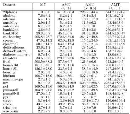
We can see that error estimates are comparable in general. However, there are several datasets where alternating model trees perform significantly better than M50model trees, and a few where they perform significantly worse. In particular, alternating model trees perform significantly worse on the puma32H data when usingλ= 1 or 0.5. Decreasing shrink-age improves error in general, in particular on the puma32H data, indicating that there is a problem with overfitting on this data. Inspection of the trees grown on various datasets shows that when λ= 1, the trees grow deep very quickly, resulting in data fragmentation and increasing the potential for overfitting. Asλis reduced, the trees become shallower. Table 2 shows average tree size, as measured by the num-ber of splitter/decision nodes. The results show that de-creasing the shrinkage parameter increases the size of the trees, i.e. cross-validation-based model selection as imple-mented usingIterativeClassif ierOptimizerperforms more iterations. Note that, just as in M50 trees, the linear regres-sion models occurring along a path in an alternating model tree can be consolidated into a single multiple linear regres-sion model stored at the leaf node associated with this path, because the sum of a set of simple linear regression models

(7)

Dataset M50 AMT AMT AMT (λ=1) (λ=0.5) (λ=0.1) 2dplanes 1.0±0.0 151.9±58.3 225.2±44.4 844.7±124.5 abalone 7.6±3.2 8.2±2.1 18.1±3.4 103.1±25.2 ailerons 5.4±1.7 33.5±7.7 78.4±17.9 467.1±113.7 autoMpg 2.9±1.5 5.4±2.2 11.3±6.3 93.4±38.6 auto-price 6.7±2.3 6.2±4.7 14.5±10.1 81.2±34.2 bank32nh 3.6±3.5 16.8±3.5 35.1±5.8 260.8±53.7 bank8FM 29.8±6.7 45.1±6.8 81.0±10.9 444.5±63.47 cal-housing 205.8±28.7 172.6±31.0 264.7±49.8 927.7±222.5 cpu-act 47.6±14.2 62.0±12.9 115.5±24.6 462.1±135.2 cpu-small 50.1±14.7 63.1±12.3 119.2±21.4 495.7±148.9 delta-ailerons 23.6±7.2 17.7±4.1 28.5±6.1 159.8±42.3 delta-elevators 6.2±2.4 12.1±2.6 26.2±4.6 133.7±24.5 diabetes-numeric 0.7±1.0 2.3±1.3 3.6±1.5 18.0±8.9 elevators 33.5±8.6 129.1±27.6 257.9±38.8 1153.5±200.5 fried 508.5±38.3 57.5±6.7 121.6±6.6 673.2±40.5 house-16H 181.1±48.1 37.8±11.6 48.6±15.4 208.6±74.3 house-8L 126.1±28.0 33.5±7.2 58.5±14.9 247.3±93.1 housing 12.0±5.3 4.3±6.6 13.0±18.6 73.4±72.6 kin8nm 108.7±18.0 263.4±36.1 527.4±61.1 2927.8±377.7 machine-cpu 2.7±1.5 5.3±5.9 12.8±7.1 74.1±32.8 mv 9.1±0.3 363.6±119.9 523.6±286.5 2232.3±866.7 pol 169.5±19.6 89.6±24.9 196.4±62.5 1047.6±330.9 puma32H 103.9±21.8 86.0±27.2 145.3±39.8 998.3±305.24 puma8NH 27.0±4.5 16.3±1.4 29.5±2.8 198.4±32.8 pyrim 1.3±1.0 3.4±6.1 7.5±6.7 51.4±37.3 servo 5.1±1.6 13.6±16.5 36.1±117.3 176.6±166.4 stock 43.7±7.5 49.2±12.5 86.4±18.3 441.9±93.4 triazines 2.7±1.3 5.7±4.2 12.3±7.9 79.9±47.9 wisconsin 2.2±2.9 0.8±0.7 1.6±1.0 12.1±8.8

Table 2: Average number of splitter nodes, estimated using 10×10-fold cross-validation

Dataset Outer CV Inner CV Outer CV Inner CV

(λ=1) (λ=0.5) 2dplanes 1.0291±0.0227 1.0325±0.0116 1.0154±0.0136 1.0165±0.0050 abalone 2.1765±0.1322 2.1760±0.0175 2.1860±0.1489 2.1883±0.0223 ailerons 0.0002±0.0000 0.0002±0.0000 0.0002±0.0000 0.0002±0.0000 autoMpg 2.8265±0.4974 2.9106±0.1146 2.8838±0.7388 2.8713±0.1031 auto-price 2345.9±947.96 2375.7±206.05 2095.4±934.33 2102.4±197.13 bank32nh 0.0826±0.0035 0.0827±0.0005 0.0822±0.0034 0.0823±0.0005 bank8FM 0.0303±0.0010 0.0304±0.0002 0.0296±0.0009 0.0297±0.0002 cal-housing 49426.±2117.7 49654.±441.43 49207.±2648.1 49052.±404.43 cpu-act 2.4352±0.2096 2.4376±0.0617 2.5078±1.0848 2.3680±0.0454 cpu-small 2.8872±0.1708 2.8882±0.0717 2.8713±0.7162 2.8271±0.0475 delta-ailerons 0.0002±0.0000 0.0002±0.0000 0.0002±0.0000 0.0002±0.0000 delta-elevators 0.0014±0.0000 0.0014±0.0000 0.0014±0.0000 0.0014±0.0000 diabetes-numeric 0.6591±0.2513 0.6092±0.0575 0.5936±0.2268 0.5876±0.0358 elevators 0.0022±0.0001 0.0022±0.0000 0.0021±0.0001 0.0021±0.0000 fried 1.0105±0.0118 1.0117±0.0021 1.0086±0.0110 1.0093±0.0014 house-16H 37361.±7601.3 35647.±545.93 35609.±3811.1 35180.±590.30 house-8L 31724.±2056.8 31486.±350.37 31277.±1990.9 31170.±367.68 housing 5.5683±4.6668 4.3045±0.3692 5.2818±3.4914 4.6027±0.5248 kin8nm 0.1170±0.0034 0.1182±0.0011 0.1091±0.0031 0.1109±0.0009 machine-cpu 63.466±29.309 65.233±9.6004 49.436±26.409 53.887±7.8728 mv 0.0064±0.0019 0.0065±0.0008 0.0615±0.3890 0.0235±0.0055 pol 9.6527±2.2639 9.3432±0.4544 8.0089±2.3251 7.6774±0.3870 puma32H 0.0204±0.0055 0.0213±0.0022 0.0135±0.0076 0.0155±0.0037 puma8NH 3.1872±0.0844 3.1876±0.0114 3.2019±0.0828 3.2029±0.0105 pyrim 0.1261±0.0748 0.1208±0.0159 0.1046±0.0679 0.1109±0.0160 servo 0.4964±0.3067 0.5413±0.1118 0.4875±0.2905 0.5298±0.0978 stock 1.0138±0.2016 1.0119±0.0645 0.8645±0.1234 0.8878±0.0460 triazines 0.1503±0.0401 0.1449±0.0088 0.1370±0.0379 0.1348±0.0083 wisconsin 34.482±4.1926 34.045±0.8672 33.486±4.0019 33.388±0.6931

Table 3: Root mean squared error obtained using outer 10×10-fold cross-validation, for AMT (λ = 1 and λ= 0.5), vs. average root mean squared error of the same model in inner 10-fold cross-validation

(8)

is a multiple linear regression model.3

It is also interesting to compare the cross-validation esti-mates obtained using inner cross-validation on the training data, encountered when selecting the “best” number of it-erations to perform, with those established from the outer 10×10-fold cross-validation used to obtain an unbiased er-ror estimate. Table 3 shows this for λ = 1 and λ = 0.5, based on root mean squared error rather than root rela-tive squared error. Note that the estimates from the inner cross-validation runs are averages over the 10×10-fold outer cross-validation runs, one for each train/test split occurring in the outer cross-validation. Thus, they are averages ob-tained from 1,000 train/test splits of the full data. As can be seen, the estimates are quite close: the average estimate obtained using inner cross-validation is always well within one standard deviation of the estimate from the outer cross-validation. This means that when building an alternating model tree withIterativeClassif ierOptimizerin practice, the cross-validation estimate associated with the number of iteration it chooses can be used as an indicator of perfor-mance on new data. This is helpful because no separate, outer evaluation process is necessary to get an indication of error on fresh data.

5. CONCLUSIONS

Model trees have proven to be a useful technique in prac-tical regression problems. In this paper, we present alternat-ingmodel trees grown using forward stagewise additive mod-eling and show that they achieve significantly lower squared error than M50 model trees on several regression problems.

In contrast to alternating decision trees for classification, our alternating model trees have prediction nodes contain-ing simple linear regression models.To reduce computational complexity and data fragmentation when constructing split-ter nodes, splits are taken to be the median value of an ap-propriately chosen attribute. Moreover, shrinkage is used to combat overfitting.

The size of the tree depends on the number of iterations of forward stagewise additive modeling that are performed. In our experiments, we have chosen this parameter using internal cross-validation. Our results indicate that the per-formance estimate obtained in this manner is close to the actual performance for all datasets considered in our ex-periments. Therefore, no external cross-validation run is required in order to establish an estimate of expected per-formance on fresh data.

References

[1] K. Bache and M. Lichman. UCI machine learning repos-itory, 2013.

[2] B. Bhattacharya and D. P. Solomatine. Neural networks and M5 model trees in modelling water level-discharge relationship. Neurocomputing, 63:381–396, 2005. [3] W. Buntine. Learning classification trees.Statistics and

Computing, 2(2):63–73, 1992.

[4] A. Etemad-Shahidi and J. Mahjoobi. Comparison be-tween M5 model tree and neural networks for prediction of significant wave height in Lake Superior. Ocean En-gineering, 36(15):1175–1181, 2009.

3

But not the least-squares multiple linear regression model.

[5] Y. Freund and L. Mason. The alternating decision tree learning algorithm. InProc 16th International Conf on Machine Learning, pages 124–133, San Francisco, CA, USA, 1999. Morgan Kaufmann Publishers Inc. [6] J. Friedman, T. Hastie, and R. Tibshirani. Additive

logistic regression: a statistical view of boosting. The Annals of Statistics, 28(2):337–407, 04 2000.

[7] M. Hall, E. Frank, G. Holmes, B. Pfahringer, P. Reute-mann, and I. H. Witten. The WEKA data mining soft-ware: an update. SIGKDD Explorations, 11(1):10–18, 2009.

[8] G. Holmes, B. Pfahringer, R. Kirkby, E. Frank, and M. Hall. Multiclass alternating decision trees. In Proc 13th European Conf on Machine Learning, Helsinki, Finland, pages 161–172. Springer, 2002.

[9] R. Kohavi and C. Kunz. Option decision trees with majority votes. In Proc 14th International Conf on Machine Learning, pages 161–169, San Francisco, CA, USA, 1997. Morgan Kaufmann Publishers Inc. [10] D. Lubinsky. Tree structured interpretable regression.

In D. Fisher and H.-J. Lenz, editors, Learning from Data, volume 112 ofLecture Notes in Statistics, pages 387–398. Springer New York, 1996.

[11] D. Malerba, F. Esposito, M. Ceci, and A. Appice. Top-down induction of model trees with regression and split-ting nodes.IEEE Transactions on Pattern Analysis and Machine Intelligence, 26(5):612–625, 2004.

[12] C. Nadeau and Y. Bengio. Inference for the generaliza-tion error. Machine Learning, 52(3):239–281, 2003. [13] E. Ould-Ahmed-Vall, J. Woodlee, C. Yount, K. A.

Doshi, and S. Abraham. Using model trees for computer architecture performance analysis of software applica-tions. In IEEE International Symposium on Perfor-mance Analysis of Systems & Software, 2007. ISPASS 2007., pages 116–125. IEEE, 2007.

[14] M. Pal and S. Deswal. M5 model tree based modelling of reference evapotranspiration.Hydrological Processes, 23(10):1437–1443, 2009.

[15] J. R. Quinlan. Learning with continuous classes. In

Proc 5th Australian Joint Conf on Artificial Intelli-gence, pages 343–348, Singapore, 1992. World Scien-tific.

[16] D. P. Solomatine and K. N. Dulal. Model trees as an alternative to neural networks in rainfall-runoff mod-elling. Hydrological Sciences Journal, 48(3):399–411, 2003.

[17] M. Taghi Sattari, M. Pal, H. Apaydin, and F. Ozturk. M5 model tree application in daily river flow forecasting in Sohu Stream, Turkey. Water Resources, 40(3):233– 242, 2013.

[18] Y. Wang and I. H. Witten. Inducing model trees for continuous classes. InProc 9th European Conf on Ma-chine Learning Poster Papers, pages 128–137, 1997.

Alternating model trees