M M Correia and J Kang and S A Richardson
Asset volatility
Article
This version is available in the LBS Research Online repository:
http://lbsresearch.london.edu/
860/
Correia, M M and Kang, J and Richardson, S A
(2018)
Asset volatility.
Review of Accounting Studies, 23 (1). pp. 37-94. ISSN 1380-6653
DOI:
https://doi.org/10.1007/s11142-017-9431-1
Reuse of this item is allowed under the Creative Commons licence:
http://creativecommons.org/licenses/by-nc/4.0/
Kluwer
https://link.springer.com/article/10.1007%2Fs11142...
Users may download and/or print one copy of any article(s) in LBS Research Online for purposes of
research and/or private study. Further distribution of the material, or use for any commercial gain, is
not permitted.
Asset volatility
Maria Correia1&Johnny Kang2&Scott Richardson3
#The Author(s) 2017. This article is an open access publication
Abstract We examine whether fundamental measures of volatility are incremental to market-based measures of volatility in (i) predicting bankruptcies (out of sample), (ii) explaining cross-sectional variation in credit spreads, and (iii) explaining future credit excess returns. Our fundamental measures of volatility include (i) historical volatility in profitability, margins, turnover, operating income growth, and sales growth; (ii) disper-sion in analyst forecasts of future earnings; and (iii) quantile regresdisper-sion forecasts of the interquartile range of the distribution of profitability. We find robust evidence that these fundamental measures of volatility improve out-of-sample forecasts of bankruptcy and help explain cross-sectional variation in credit spreads. This suggests that an analysis of credit risk can be enhanced with a detailed analysis of fundamental information. As a test case of the benefit of volatility forecasting, we document an improved ability to forecast future credit excess returns, particularly when using fundamental measures of volatility.
Keywords credit spreads . volatility . bankruptcy . default
JEL classification G12 . G14 . M41 https://doi.org/10.1007/s11142-017-9431-1 * Maria Correia [email protected] Johnny Kang [email protected] Scott Richardson [email protected] 1
London School of Economics and Political Science, London, UK
2 BlackRock, New York, USA
3
1 Introduction
Fixed income markets are enormous. As of Dec. 31, 2016 over $45 trillion of investment grade bonds were included in the Barclays/Bloomberg Global Aggregate Index (AGG). Out of the AGG, roughly $10 trillion represents bonds issued by investment grade-rated companies from developed markets. In addition, there is about $1.5 trillion of corporate bonds outstanding that have been issued by high yield-rated companies from developed markets. Together, investment-grade and high-yield corpo-rate credits comprise a very large market, and to date, little research has explored the role of fundamental analysis in the context of credit markets.
The key risk in credit markets is default. Investors who are long credit claims are exposed to the risk that the issuer will default before making all of the contractual payments required by the credit instrument. The workhorse model in understanding how the risk of default links to security prices in credit markets is the work of Merton (1974). In this structural model, volatility is arguably the most important primitive variable for determining default risk. While there are many variants of structural models, a theme is that a firm will default if its asset value is below a default threshold at some future point. Thus structural models provide a framework to quantify the probability that a firm will have an insufficient asset value to satisfy its debt commitments. A firm’s closeness to the default threshold is a function of both (i) the expected difference between asset values and debt commitments and (ii) volatility. For a given asset value and capital structure today, higher expected volatility implies a greater probability that future asset values will not cover debt commitments (i.e., a greater chance of default).1
Our objective is to conduct a comprehensive empirical analysis of the usefulness of market-based and fundamental-based measures of volatility from the perspective of a credit investor. The FASB recognizes the potential usefulness of fundamental informa-tion contained in general purpose financial reports for both equityanddebt investors. We focus on the latter group. While there is a rich literature examining how accounting data can be used to help forecast corporate bankruptcy and default (e.g., Beaver1966; Altman1968; Ohlson1980; Beaver et al.2005; Bharath and Shumway2008; Campbell et al.2008; Correia et al.2012), there is scant analysis of how fundamental measures of risk can be used to improve credit-related investment decisions. Most of these studies use a mix of fundamental and market-based variables to predict bankruptcy, but a theme in this research is the central importance of market-based measures of volatility. A recent notable exception is the work of Konstantinidi and Pope (2016), who document that quantile-based forecasts of the risks embedded in accounting rates of return can help explain credit ratings and spreads. Our focus is on whether information from the accounting system could be additive to market-based measures of volatility in helping investors in the credit markets quantify default risk and how that risk is priced. While it is clear that measuring asset volatility is key for credit markets, it is ultimately an empirical question as to whether and how measures of asset volatility derived from financial statement data can be additive to market-based measures of asset volatility. At a minimum, the information contained in historical volatility of fundamentals (e.g., accounting rates of return) differs from market-based measures. Financial statements
1
Other studies using a structural approach to explain credit spreads include those by Crouhy et al. (2000); Eom et al. (2004); Arora et al. (2005); Cremers et al. (2008); Zhang et al. (2009); and Correia et al. (2012).
are prepared under modified historical cost accounting (not full mark to market). Penman (2016) suggests that the unconditional conservatism built into financial reporting creates the possibility of risk to be reflected in the outputs of that system. It is volatility in these outputs that we examine.
We source our market-based measures of asset volatility from traded security prices in secondary markets. We derive several measures of historical asset volatility, ranging from a simple deleveraging of historical equity volatility to a complete measure that uses historical equity and credit return volatilities and historical return correlations (e.g., Schaefer and Strebulaev2008). We also combine forward-looking market information using the implied volatility from at-the-money put and call options. Our fundamental-based measures of volatility are obtained from the primary financial statements and are designed to capture fundamental volatility in unlevered profitability. We use a wide range of fundamental volatility measures, including (i) historical volatility in profitabil-ity, margins, turnover, operating income growth, and sales growth; (ii) dispersion in analyst forecasts of future earnings; and (iii) quantile regression forecasts of the inter-quartile range of the distribution of profitability (e.g., Konstantinidi and Pope2016).
Our empirical analysis is comprised of three main sections. First, we examine the relative importance of market- and fundamental-based measures of asset volatility to forecast (out-of-sample) bankruptcy and default. For a large sample of U.S. firms from 1989 to 2012 using traditional discrete-hazard modelling and classification and regres-sion trees (CART) methodology, which allows for nonlinear and interactive associa-tions between probability of default and different explanatory variables, we find that combining information about volatility from market and fundamental sources improves forecasts of corporate bankruptcy. Our bankruptcy prediction models are superior to the standard models in at least two respects. First, we demonstrate improvement in out-of-sample classification accuracy, which is typically not reported (e.g., Altman 1968; Ohlson1980; Bharath and Shumway2008; Campbell et al. 2008). Second, we show that combining multiple measures of volatility generates superior forecasts, relative to prevailing bankruptcy forecasting models (e.g., Campbell et al.2008).
Second, we assess the relative importance of market- and fundamental-based measures of asset volatility to explain cross-sectional variation in credit spreads. Assuming markets are reasonably efficient with respect to the usefulness of market- and fundamental-based measures of volatility in forecasting (out-of-sample) bankruptcies, these measures should also help explain variation in credit spreads. Using traditional unconstrained linear regression analysis and CART, which allows for various nonlinear and interactive effects, we find that combining market- and fundamental-based volatility estimates improves explanatory power of cross-sectional credit spreads, although the market-based measures appear to dominate fundamental measures. This analysis is robust to a broad cross-section of corporate bond spreads from 1992 to 2012 as well as CDS spreads from 2004 to 2012. We extend this analysis by using market- and fundamental-based measures of asset volatility within the structural model of Merton (1974). This constrained use of asset volatility significantly improves our ability to explain cross-sectional variation in credit spreads. This is because the relation between leverage and asset volatility and default risk and hence credit spreads is inherently nonlinear. For the constrained analysis, we continue to find robust evidence that combining market- and fundamental-based volatility estimates improves explanatory power of cross-sectional credit spreads, but again the market-based measures appear to dominate.
Third, we explore the relative importance of market- and fundamental-based mea-sures of asset volatility to forecast future credit excess returns. We undertake this analysis given the somewhat surprising result from our first two sets of analyses. In the first set of empirical tests, we find that both market- and fundamental-based measures of asset volatility are important to forecast bankruptcy, but in our second set of analyses, market-based measures tend to dominate. This raises the possibility that credit markets are not paying enough attention to fundamental-based measures. Using the regression framework from Correia et al. (2012), we assess whether measures of credit risk mispricing (the difference between observed credit spreads and modelled credit spreads using either market- or fundamental-based measures of asset volatility) help predict credit excess returns. If the market is not paying enough attention to fundamental measures of asset volatility, we would expect to see measures of credit risk mispricing based on fundamental asset volatility better predict credit excess returns. Using a large sample of corporate bonds from 1996 to 2012, we find results consistent with this hypothesis.
Overall, our paper fits into the broad default forecasting literature and the more recent literature linking fundamental analysis to asset pricing attributes from the credit market (both spreads and returns). The paper also relates, more broadly to the risk ratings (e.g., Liu et al.2007) and to the credit ratings literatures (e.g., Kraft2014). Our results speak to the relevance of fundamental analysis from the perspective of a credit investor. While our focus is on measuring asset volatility using fundamental information, there are additional aspects of financial statement information that also matter from the perspec-tive of a credit investor, including measuring different aspects of leverage: on and off balance sheet financial leverage as well as operating leverage. Given the growing size and importance of credit markets globally, we hope that future research can continue to explore the relevance of financial statement information for credit valuation.
The rest of the paper is structured as follows. Section 2 describes our sample selection and research design. Section3presents our empirical analysis and robustness tests, and section4concludes.
2 Sample and research design
2.1 Secondary credit market dataOur analysis is based on a comprehensive panel of U.S. corporate bond data, which includes all the constituents of (i) Barclays U.S. Corporate Investment Grade Index and (ii) Barclays U.S. High Yield Index. The data includes monthly returns and bond characteristics from September 1988 to February 2013. We exclude financial firms with SIC codes between 6000 and 6999.
2.2 Representative bond
Given that corporate issuers often issue multiple bonds and that our analysis is directed at measuring asset volatility of the issuer, we need to select a representative bond for each issuer. To do this, we follow the criteria of Haesen et al. (2013). We repeat this exercise every month for our sample period. The criteria used for identifying the
representative bond are selected so as to create a sample of liquid and cross-sectionally comparable bonds. Specifically, we select representative bonds on the basis of (i) seniority, (ii) maturity, (iii) age, and (iv) size.
First, we filter bonds by seniority. Because most companies issue the majority of their bonds as senior debt, we select only bonds corresponding to the largest rating of the issuer. To do this, we first compute the amount of bonds outstanding for each rating category for a given issuer. We then keep only those bonds that belong to the rating category that contains the largest fraction of debt outstanding. These bond tends to have the same rating as the issuer. Second, we then filter based on maturity. If the issuer has bonds with time to maturity between 5 and 15 years, we remove all other bonds for that issuer from the sample. If not, we keep all bonds in the sample. Third, we then filter based on time since issuance. If the issuer has any bonds that are at most two years old, we remove all other bonds for that issuer. If not, we keep all bonds from that issuer in the sample. Finally, we filter based on size. Of the remaining bonds, we pick the one with the largest amount outstanding.2
Our resulting sample includes 121,300 unique bond-month observations, corre-sponding to 5362 bonds issued by 1504 unique firms. Table1 Panel A shows the industry composition of the sample, using Barclays Capital’s industry definitions. Approximately 35% of the sample firms are consumer products firms. Capital goods firms and basic industry make up another 20% of the sample. Sample bonds have an average option-adjusted spread (OAS) of 3.31% over the sample period and an average option adjusted duration of 5.16 years (Table1, Panel B). AppendixIdefines these variables as well as other variables used in the paper in more detail.
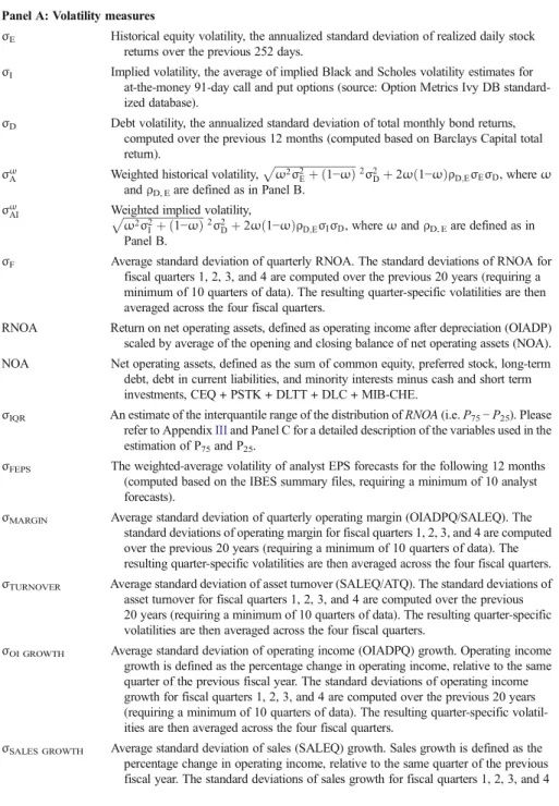
2.3 Measures of asset volatility 2.3.1 Historical market data
We calculate historical equity volatility using the annualized standard deviation of CRSP realized daily stock returns over the past 252 days,σE. We combine historical credit and equity market data to obtain our first measure of asset volatility,σωA:
σω A¼ ffiffiffiffiffiffiffiffiffiffiffiffiffiffiffiffiffiffiffiffiffiffiffiffiffiffiffiffiffiffiffiffiffiffiffiffiffiffiffiffiffiffiffiffiffiffiffiffiffiffiffiffiffiffiffiffiffiffiffiffiffiffiffiffiffiffiffiffiffiffiffiffiffiffiffiffiffiffi ω2σ2 Eþð1−ωÞ 2σ2 Dþ2ωð1−ωÞρD;EσEσD; q ð1Þ whereωis the ratio of the market value of the firm’s equity to the total firm value,
σDis the annualized standard deviation of total monthly bond returns, andρD,Eis 2For example, Basic Energy Services, Inc. has two bonds in the Barclays Capital bond sample with return
information for October 2009, one with rating BA3 and another with rating CAA1. We first compute the fraction of debt outstanding for each rating. In this case, half of the debt is rated BA3, and the other half CAA1, as the bonds have the same amount outstanding of $225,000. Therefore both bonds are kept in the sample after the first step. The second selection step is based on years to maturity. The first bond has 4.75 years to maturity, and the second bond 6.46. We drop the first bond as time to maturity is lower than five, and therefore the second bond is selected as the representative bond. Viacom Inc. has five bonds in the sample in December 2012, all with the same rating of BAA1. Two of these bonds have time to maturity between 5 and 15 years. Therefore we remove the remaining three bonds from the sample. Both bonds were issued at the same time. They are both 1.36 years old. Therefore we select the representative bond based on amount outstanding. Similar bond selection criteria are used by Correia et al. (2012) and Cascino (2017).
Ta b le 1 Descriptive stat istics Panel A : In dustr y com position % Cons ume r Nonc yc lic al 17 .35 Cons ume r Cy cli ca l 17 .21 Cap ita l G oo ds 10 .41 Bas ic Ind ust ry 1 0 .16 Ene rgy 9 .77 Comm uni ca tion s 9 .03 Elect ric 8.14 T ech nol ogy 6 .36 Othe r Ind u str ia l 4 .4 6 T ra n sp ort ati on 3 .38 Natural G as 2.53 Other 1 .20 Pa nel B : B o n d cha ra ct er ist ic s N M ea n S td . D ev . p 1 p 25 Med ian p 7 5 p 9 9 OAS 12 1,30 0 0 .0 331 0 .05 13 0. 000 0 0 .0 096 0. 019 4 0 .040 0 0 .2 419 Dur at ion 12 1,28 7 5 .1 558 2 .19 96 0. 710 0 4 .0 300 5. 000 0 5 .960 0 1 2.5 800 Age 1 19, 463 2.8 927 2 .43 65 0.1 1 7 8 1.1 562 2. 400 0 3 .989 0 1 2.7 096 Rat ing 12 0,89 2 1 0.3 646 4 .03 74 2. 000 0 7 .0 000 1 0 .0 000 14. 000 0 1 9.0 000 Exr et 1 2 1 ,26 8 0.0 020 0 .12 69 − 0. 329 5 − 0.0 538 − 0 .00 1 1 0. 052 6 0 .3 727 ln V X 12 1,25 4 1 .8 238 0 .73 26 0. 633 2 1 .2 785 1. 709 0 2 .256 1 3 .9 473 ln (E) 1 2 1 ,30 0 7.9 820 1 .69 74 3. 680 2 6 .9 013 8 .01 1 5 9. 129 9 1 1.8 345 ω 12 1,30 0 0 .6 348 0 .22 12 0. 065 2 0 .4 944 0. 669 1 0 .81 1 4 0 .9 712
Ta b le 1 (c o n tin ue d) r 2 i;t 121 ,156 0. 206 3 0 .156 6 0 .0 005 0 .08 03 0.1 764 0 .30 25 0. 627 6 ρE, D 121 ,300 0. 219 4 0 .151 1 0 .0 500 0 .07 29 0.1 894 0 .33 95 0. 570 8 Panel C : V olat ili ty me asur es N M ea n S td. D ev . p 1 p 25 Median p75 p 99 σE 120 ,034 0. 408 2 0 .237 2 0 .1 31 1 0 .24 9 7 0 .344 6 0 .48 8 5 1 .295 3 σI 92,9 3 9 0 .390 3 0 .190 8 0 .1 434 0 .26 03 0. 344 5 0 .46 4 8 1 .085 0 σD 92,6 3 4 0 .088 6 0 .104 9 0 .0 140 0 .04 28 0. 058 1 0 .08 7 3 0 .606 5 σ ω A 92,1 3 9 0 .256 2 0 .137 6 0 .0 781 0 .16 63 0. 225 0 0 .30 7 4 0 .778 7 σ ω AI 71,3 9 2 0 .258 1 0 .1 178 0.0 820 0 .17 94 0. 236 5 0 .30 9 8 0 .676 1 σF 100 ,318 0. 033 1 0 .045 7 0 .0 051 0 .01 35 0. 021 2 0 .03 4 4 0 .287 6 σIQR 11 7,9 2 6 0 .040 7 0 .037 1 0 .0 061 0 .02 23 0. 033 0 0 .04 5 8 0 .228 3 σFEPS 63,2 7 4 0 .234 9 5 .512 9 0 .0 075 0 .03 67 0. 075 8 0 .17 0 0 1 .480 0 σMA RG IN 101 ,541 0. 185 9 0 .480 1 0 .0 134 0 .05 77 0. 090 2 0 .14 6 4 1 .903 8 σTU R N O V E R 100 ,464 0. 681 3 3 .1 1 1 3 0 .0 251 0 .1 1 8 5 0. 209 5 0 .40 0 9 1 0 .57 76 σOI GRO W TH 98,9 9 1 1 .161 1 0 .694 5 0 .2 144 0 .56 40 1. 022 0 1 .63 9 7 2 .879 3 σSALES GR OWTH 98,9 0 8 0 .409 0 0 .249 9 0 .0 978 0 .22 59 0. 348 8 0 .52 4 6 1 .314 4 Pan el D : C o rr elat ion s a cross vol ati lit y m ea sures σE σI σD σ ω A σ ω AI σF σIQR σFEPS σMA RG IN σTUR N OVE R σOI GR OW TH σSALE GRO W TH σE 1 0 .881 4 0 .432 9 0 .7 109 0 .67 57 0. 190 8 0 .09 3 8 0 .220 2 0 .1 833 0 .061 3 0 .47 1 3 0 .3 285 σI 0.90 05 1 0 .487 8 0 .6 006 0 .70 18 0. 179 5 0 .1 14 6 0 .232 8 0 .2 121 0 .052 1 0 .48 5 3 0 .3 365 σD 0.30 64 0. 337 7 1 0.2 652 0 .29 87 0. 059 6 0 .06 1 6 0 .108 5 0 .1 001 0 .014 5 0 .22 4 0 0 .1 514 σ ω A 0.70 97 0. 626 7 0 .145 8 1 0 .91 69 0. 268 8 0 .29 5 9 0 .094 0 0 .1 227 0 .091 8 0 .30 9 7 0 .1 739 σ ω AI 0.66 53 0. 716 2 0 .164 7 0 .9 173 1 0 .276 3 0 .31 1 5 0 .131 1 0 .1 533 0 .090 9 0 .34 4 2 0 .1 945 σF 0.35 93 0. 350 3 0 .084 4 0 .4 21 1 0 .43 3 2 1 0 .42 00 0. 035 9 0 .2 530 0 .671 7 0 .27 8 5 0 .2 743
Ta b le 1 (c o n tin ue d) σIQR − 0 .00 36 0. 012 5 − 0. 041 8 0 .2 901 0 .30 61 0. 266 6 1 − 0.0 363 0 .05 57 0. 289 2 − 0 .06 70 − 0.0 644 σFEPS 0 .28 95 0. 319 1 0 .133 1 0 .0 942 0 .12 90 0. 132 1 − 0 .20 07 1 0 .16 1 8 − 0. 01 14 0 .36 78 0.1 460 σMA RG IN 0 .18 15 0. 198 1 0 .100 0 0 .0 432 0 .07 25 0. 360 9 − 0 .03 68 0.2 809 1 0 .008 7 0 .40 4 9 0 .5 223 σTU R N OV E R 0 .24 17 0. 229 1 0 .046 4 0 .2 705 0 .27 06 0. 614 3 0 .174 5 − 0.0 410 − 0 .16 65 1 0 .1 12 8 0 .1 095 σOI GROWTH 0 .49 73 0. 521 6 0 .200 4 0 .2 713 0 .31 07 0. 478 6 − 0 .17 76 0.4 923 0 .52 35 0. 226 7 1 0.5 869 σSALES G ROWTH 0 .34 05 0. 356 6 0 .144 1 0 .1 558 0 .17 55 0. 339 5 − 0 .15 00 0.2 696 0 .47 21 0. 223 2 0 .61 6 1 1 Pane l E : C or re la ti ons b et wee n ac tual and implie d cr edi t spr ea ds OAS C S BAS E σE CS σE CS σI CS σ ωA CS σ ωAI CS σF CS σAV G CS PR O BAVG OAS 1 0 .738 2 0 .781 3 0 .7 521 0 .77 17 0. 761 0 0 .628 8 0 .7 218 0 .71 25 CS BA SE σE 0 .74 63 1 0 .981 1 0 .9 194 0 .84 15 0. 827 3 0 .717 6 0 .8 175 0 .80 23 CS σE 0 .75 18 0. 999 1 1 0.9 442 0 .88 49 0. 868 1 0 .751 0 0 .8 608 0 .83 99 CS σI 0 .71 73 0. 959 0 0 .960 4 1 0 .84 86 0. 895 7 0 .764 8 0 .8 624 0 .84 32 CS σ ω A 0 .70 62 0. 895 7 0 .898 1 0 .8 417 1 0 .944 9 0 .699 0 0 .7 951 0 .77 32 CS σ ωAI 0 .68 35 0. 858 0 0 .861 1 0 .9 021 0 .93 37 1 0 .691 0 0 .7 705 0 .75 73 CS σF 0 .57 81 0. 759 1 0 .762 5 0 .7 540 0 .57 19 0. 569 3 1 0.8 825 0 .90 96 CS σAV G 0 .63 52 0. 815 2 0 .817 3 0 .8 094 0 .60 73 0. 603 5 0 .931 9 1 0 .97 90 CS PR OB AV G 0 .59 77 0. 773 0 0 .775 5 0 .7 633 0 .58 52 0. 579 1 0 .934 2 0 .9 787 1 Panel A report s the industry compos itio n o f the sampl e, u si ng the F ama F rench 1 2-i ndustry clas si fi cation. Panel B reports d es cripti ve st ati stics fo r b o n d an d iss u er cha rac ter ist ics . Pa ne l C reports descriptive statis tics for th e d if ferent market and fundamental v olatili ty measures. P an el D reports correl ati ons acros s volatil ity mea su re s. Pan el E re po rts cor re lat ion s b et wee n ac tua l an d im p lie d cre di t spr ea ds . C orr el ati ons ar e comp u te d for ea ch o f th e m ont hs wit h av ai lab le d at a b as ed on the la rge st po ssib le sam ple siz e for eac h p air o f d ef au lt fo re ca sts. Re por te d corr elat ions ar e ave ra ge s ac ross the m ont hs in the sam ple . A v er ag e P ea rs o n (Spe ar ma n) cor re la tio ns ar e re por te d abov e (bel o w) th e d ia gon al an d av er ag e. V aria b le de fin itio ns ar e p ro vide d in A p p en dix I
an estimate of the historical correlation between equity and bond returns. Note that, while our selection of a representative bond can change each month for a given issuer, our correlation and volatility measures hold a given bond fixed when looking back in time.
Table1 Panel B presents descriptive statistics for the variables used to compute asset volatility. Sample firms have an average market leverage of approximately 36% (1–0.6348) and exhibit an average correlation between equity and debt returnsρD, E of 0.2194.
2.3.2 Forward-looking market data
We obtain Black-Scholes implied volatility estimates for at-the-money 91-day options from the OptionMetrics Ivy DB standardized database.3We average the implied volatility for a 91-day put and call option. Based on this implied equity volatility,σI, we computeσωAI, using the approach in (1). Option implied volatility has been shown to have incremental power with respect to historical volatility in explaining time-series and cross-sectional variation in credit spreads (Cremers et al.2008b; Cao et al.2010).
2.3.3 Fundamental data
Following Penman (2014), we use return on net operating assets (RNOA) as the measure of unlevered (or enterprise) profitability. For each quarter, we compute RNOA as operating income (OIADPQ) to average net operating assets (NOA) during the quarter.
We construct a simple fundamental volatility measure,σF, based on the historical volatility of quarterly RNOA, which we then average across fiscal quarters to remove the effects of seasonality. Specifically, we computeσFas:
σF ¼ ∑
4
k¼1
Std RNOAð kÞ
4 ; ð2Þ
whereStdk(RNOAitk) is the standard deviation of RNOA for quarter k calculated over
the previous 20 quarters, requiring a minimum of 10 quarters of data. We annualizeσF,
by multiplying the average standard deviation bypffiffiffi4.
Our second fundamental volatility measure,σIQR, is based on an estimate of the interquartile range of the distribution of profitability, which is obtained using a quantile regression approach (Konstantinidi and Pope2016). This approach, which is described in detail in Appendix III, has the advantage of not requiring time series data for computation as it relies only on cross-sectional fundamental characteristics.
Our third fundamental volatility measure is based on the dispersion of analysts’ earnings forecasts. The dispersion of analysts’earnings forecasts may be regarded as a proxy for future earnings (fundamental) uncertainty. We obtain the standard deviations of analyst EPS forecasts for the following two fiscal years (σFEPS1, 3
The standardized implied volatilities are calculated by OptionMetrics using linear interpolation from their Volatility Surface file.
σFEPS2) from the IBES Summary database and compute a weighted average
standard deviation as follows:
σFEPS¼ασFEPS1þð1−αÞσFEPS2; ð3Þ
whereαis the number of months to the end of the current fiscal year divided by 12.
Based on the Dupont decomposition of profitability into profit margin and asset turnover, we further compute the volatility of operating margins (the ratio of operating income to sales) and asset turnover (the ratio of sales to total assets). Similarly toσF, these volatilities,σMARGIN and σTURNOVER, represent an average of quarter-specific volatilities. We calculate two additional fundamental volatility measures, the volatility of operating income growth (σOI GROWTH) and the volatility of sales growth (σSALES
GROWTH). Operating income (sales) growth is defined as the percentage change in
operating income (sales), relative to the same quarter of the previous year.
2.3.4 Correlations across volatility measures
Table1Panel C reports descriptive statistics for the different volatility measures. We winsorize all volatility measures at the 1st and 99th percentile values of their respective distributions. These measures exhibit differences in scale. We discuss how we deal with differences in scale when using different measures of asset volatility to derive implied credit spreads in section3.2.2.
Panel D of Table1reports the average monthly pairwise correlations across vola-tility measures. Historical equity volavola-tility, σE, is highly correlated with implied volatility, σI, (0.8814 (0.9005) Pearson (Spearman) correlation). The Pearson (Spearman) correlation between these equity volatility measures and debt volatility,
σD, ranges between 0.4329 and 0.4878 (0.3064 and 0.3377), respectively. As a result, the correlations between weighted asset volatilities and the corresponding equity volatility measures are, on average, lower than 0.75. The Pearson (Spearman) correla-tions among the different fundamental volatility measures range from −0.0670 to 0.6717 (−0.2007 to 0.6161) and average 0.2152 (0.2237). Pairwise Pearson (Spearman) correlations between fundamental- and market-based asset volatility mea-sures (σωA;σωAIÞaverage 0.2042 (0.2317).
2.4 Bankruptcy data and distance to default
We estimate the probability of bankruptcy based on a large sample of Chapter 7 and Chapter 11 bankruptcies filed between 1980 and the end of 2012. We combine bankruptcy data from four main sources: Beaver et al. (2012)4; the New Generation Research bankruptcy database (bankruptcydata.com); Mergent FISD; and the UCLA-Lo Pucki bankruptcy database.
4Beaver et al. (2012) combine the bankruptcy database from Beaver et al. (2005), which was derived from
multiple sources including CRSP, Compustat, Bankruptcy.com, Capital Changes Reporter, and a list provided by Shumway with a list of bankruptcy firms provided by Chava and Jarrow and used by Chava and Jarrow (2004).
We use a discrete time-hazard model and include three types of observations in the estimation: nonbankrupt firms, years before bankruptcy for bankrupt firms, and bankruptcy years (Shumway2001). Our dependent variable equals 1 if a firm files for bankruptcy within one year of the end of the month and zero otherwise. We keep the first bankruptcy filing and remove from the sample all months after this filing.
Following Correia et al. (2012), we use quarterly financial data to compute the default barrier and update market data on a monthly basis to obtain monthly estimates of the probabilities of bankruptcy. Market variables are measured at the end of each month, and accounting variables are based on the most recent quarterly information reported before the end of the month. We winsorize all independent variables at 1% and 99%. We ensure that all independent variables are observable before the declaration of bankruptcy. Furthermore, to ensure that prediction is made out of sample and to avoid a potential bias of ex post over-fitting the data, we estimate coefficients using an expanding window approach. We convert the different scores into probabilities as follows: Prob = escore/1 +
escore. All of the models are nonlinear transformations of various fundamental
and market data.
The primary regression model for estimating bankruptcy over the next 12 months is as follows:
Pr Yð itþ1¼1Þ ¼ f ln
Vit
Xit ;
Exretit;ln Eð Þit ;P5;it;Skewit;Kurtit;σk;it
: ð4Þ
ln VitXit
is a measure of dollar distance to default barrier (akin to an inverse measure of leverage). We computeVitas the sum of the market value of the firm’s equity and the
book value of debt. We compute our default barrier,Xit, as the sum of short-term debt
(DLCQ) and half of long-term debt (DLTTQ) as reported at the most recent fiscal quarter (e.g., Bharath and Shumway2008).Exretitis the excess equity return over the
value-weighted market return over the previous 12 months. ln(Eit) is the logarithm of
the market value of equity measured at the start of the forecasting month.P5,itis an
estimate of the 5th percentile of the distribution of RNOA. It is calculated as described in AppendixIII, using the quantile regressions employed by Konstantinidi and Pope (2016).P5,itis a measure of left-tail risk in profitability. Skewitis an estimate of the
skewness of the distribution of RNOA. Following Konstantinidi and Pope (2016), we estimate skewness asðP75−P50Þ−ðP50−P25Þ
IQR , whereIQRis the interquartile range (P75−P25).
Accordingly, Skewit ranges between −1 and 1 and is zero when the distribution of RNOAis symmetric within the interquartile range. Kurtitis an estimate of the kurtosis
of the distribution of RNOA, estimated following Konstantinidi and Pope (2016) as
P87:5−P62:5
ð ÞþðP37:5−P12:5Þ
IQR .σk,it is the respective measure of asset volatility as defined in
section2.3. The choice of independent variables is based on the Merton model of credit spreads to which we add a measure of left-tail risk. We estimate equation (4) using various combinations of our measures of asset volatility over different samples to assess
the relative importance of market-based and fundamental-based measures of asset volatility in the context of forecasting bankruptcy.
Our priors for equation (4) are as follows. (i) ln Vit Xit
is expected to be negatively associated with bankruptcy likelihood (the further the market value of assets is from the default barrier the lower the likelihood of hitting that barrier in the next 12 months). (ii) Exretit is expected to be negatively associated with bankruptcy
likelihood (assuming there is information content in security prices, decreases in security prices should be associated with increased bankruptcy likelihood). (iii) ln(Eit) is expected to be negatively associated with bankruptcy likelihood (large
firms offer better diversification and better realizations of asset values in the event of default). (iv) P5,it is expected to be negatively associated with bankruptcy
likelihood (the higher the 5th percentile of the RNOA distribution, the lower the probability that asset value will fall below the book value of debt). (v) Skewit is
expected to be negatively associated with bankruptcy likelihood (the more nega-tively skewed the distribution of earnings, the higher the likelihood the asset value will fall below the book value of debt). (vi) Kurtit is expected to be positively
associated with bankruptcy likelihood (higher kurtosis indicates that the density of the tails of the distribution is higher than what would be expected under a normal distribution). (vii) σk, it is expected to be positively associated with bankruptcy likelihood (the greater the volatility of the asset value the greater the chance of passing through the default barrier).
In an alternative specification, we also control for the level of option-adjusted spreads (OASit) as a market based measure of credit risk. To the extent that credit
market participants incorporate fundamental volatility in assessing credit risk, OASitcould subsume the fundamental volatility measures.
2.5 Credit spreads
Given that a measure of asset volatility is useful in forecasting bankruptcy and under the assumption that security prices in the secondary credit market are reasonably efficient, we also test how different combinations of measures of asset volatility can explain cross-sectional variation in credit spreads. We view the analysis of credit spreads as supporting evidence for assessing the information content of fundamental- and market-based measures of asset volatility.
We do this via two approaches. First, we estimate an unconstrained cross-sectional regression where we include multiple measures of determinants of credit spreads in a linear model. Second, we estimate a constrained cross-sectional regression where we combine our various measures of asset volatility into mea-sures of distance to default, which are in turn mapped to an implied credit spread following the approach of Crouhy et al. (2000); Kealhofer (2003); and Arora et al. (2005). A benefit of the constrained approach is that it combines the dollar distance to default, ln Vit
Xit
, with measures of asset volatility, σk, it, to better identify closeness to the default threshold. An unconstrained regression cannot capture the inherent nonlinear relations between leverage, asset volatility, defaults (bankruptcy), and credit spreads.
For the unconstrained approach, we estimate the following regression model.
OASit¼α1ln
Vit
Xit þα2
Exretitþα3lnð Þ þEit α4P5;itþα5Skewitþα6Kurtit
þ ∑K
k¼1
αkþ6σk;itþΓControlitþεit: ð5Þ
OASit is the option-adjusted spread for the respective bond as reported in the
Barclays Index. An intercept is not reported as we include time fixed effects. In addition to the determinants of bankruptcy, i.e., ln Vit
Xit
, Exretit, ln(Eit), P5,it, Skewit, Kurtit, and
σk, it, which are all issuer-level determinants of credit risk, we also include
issue-specific determinants of credit risk and liquidity that will influence the level of credit spreads. Specifically, our additional controls include (i) Ratingit, the issue-specific
rating (higher rated issues are expected to have higher credit spreads, given that we code ratings to be increasing in risk), (ii) Ageit, the time since issuance in years
(liquidity is decreasing for progressively off-the-run securities, so we expect credit spreads to be increasing in time since issuance), and (iii) Durationit, the option-adjusted
duration of the issue (for the vast majority of corporate issuers the credit term structure is upward sloping so we expect credit spreads to increase with duration; see Helwege and Turner1999).
For the constrained approach, we then estimate the following regression model.
OASit¼α1Exretitþα2lnð Þ þEit α3P5;itþα4Skewitþα5Kurtitþ ∑
K
k¼1
αkþ5CSσk;it
þΓControlitþεit: ð6Þ
CSσk;it is the theoretical credit spread for the k th
measure of asset volatility. The estimation of theoretical credit spreads entails six main steps (which are described in detail in AppendixII). (1) We standardize each asset volatility measure and match its moments to the moments of weighted historical asset volatility,σωA. (2) We construct estimates of distance to default, based on each asset volatility measure. (3) We empirically map each distance-to-default measure to our bankruptcy data, using a discrete time hazard model to generate a forecast of physical bankruptcy probability (see equation (A.1) of AppendixII).5(4) We compute a cumulative physical bankruptcy probability by cumulating default probabilities over the duration of the bond. (5) We convert each cumulative physical probability measure into a risk-neutral measure, by adding a risk-premium (see equation (A.2) of Appendix II). (6) Based on this risk-neutral measure and the expected recovery rate (which is assumed to be constant), we calculate theoretical credit spread as in equation (A.3).
We obtain a different theoretical credit spread for each asset volatility measure. We estimate two additional credit spreads, CSσAVGand CSPROBAVG, based on the
combina-tion of our seven fundamental volatility measures (i.e., σF, σIQR, σFEPS, σMARGIN,
5
We estimate this model using expanding windows to ensure that all observation used in the estimation is available at timet.
σTURNOVER,σOI GROWTH,σSALES GROWTH). CSσAVGand CSPROBAVGdiffer in the way in
which the different volatilities are combined. To obtain CSσAVG, we take the average of the
seven fundamental volatility measures after step (1) above (i.e., after matching their respective moments toσωA). We then follow steps (2) to (6), using this average as a measure of fundamental volatility. In contrast, to calculate CSPROBAVG, we first follow steps (1) to (3)
to obtain estimates of the physical default probabilities corresponding to each of the seven fundamental volatility measures. We then take the average of these physical default probabilities and follow steps (4) to (6) based on this average. The average monthly correlation between CSσAVG and CSPROBAVG is above 0.9 (Table1Panel E).
CSσAVG and CSPROBAVG exhibit an average Pearson (Spearman) correlation with
market-based credit spreads ( CSσω
A;CSσωAI) of 0.7740 (0.5938) and an average Pearson
(Spearman) correlation of 0.7172 (0.6165) with observed credit spreads. The high correlation with OAS suggests that our structured use of leverage and asset volatility as outlined in AppendixIIis an effective way to aggregate market and fundamental information for credit valuation purposes.
Theoretical spreads based on historical security data or option-implied vola-tility exhibit a higher correlation with observed spreads than theoretical spreads based on fundamental accounting data. In particular, OAS exhibits an average Pearson (Spearman) correlation with market-based spreads (CSσω
A;CSσωAI) of
0.7664 (0.6946) and an average Pearson (Spearman) correlation with accounting-based spreads (CSσAVG, CSPROBAVG) of 0.7172 (0.6165). Also note
that CSσAVG and CSPROBAVGexhibit stronger correlations with OAS than CSσF.
(The Pearson (Spearman) correlation between CSσF and OAS is 0.6288
(0.5781)). This suggests that there is value to conducting a deeper financial statement analysis and combining different fundamental volatility measures.
3 Results
3.1 Bankruptcy forecasting
Table2reports the estimation results of regression equation (4). The sample size used for the basis of estimating equation (4) is 81,802 bond-month observations (in speci-fications withσIthe sample is reduced to 61,132 observations, asσIis only available from 1996 onward). The sample is further reduced in specifications that includeσFEPS and hence require availability of IBES data.
Across all specifications, we find expected relations for our primary determinants: bankruptcy likelihood is decreasing in (i) distance to default barrier, ln Vit
Xit
, (ii) recent equity returns, Exretit, and (iii) firm size, ln(Eit). The coefficients on P5, it, Skewit, and
Kurtitare insignificant across most specifications. To assess the relative importance of
our different measures of asset volatility, we first examine each measure individually after controlling for the same-issuer-level determinants of bankruptcy. Across models (1) to (6) in Table2, we find that all of the measures of asset volatility are significantly positively associated with the probability of bankruptcy.
To provide a sense of the relative economic significance across the different measures of asset volatility, we report in Panel B of Table2the marginal effects for
Ta b le 2 Probabi lity of ba nkrupt cy Pr Yit þ 1 ¼ 1 ðÞ ¼ fl n Vit Xit ; Exret it ; ln Eit ðÞ ; P5; it ; Sk ew it ; Ku rtit ; σk;it hi (4 ) Panel A : R egr ession analysis (1) (2 ) (3) (4) (5) (6) (7 ) (8) (9) (10) (1 1 ) (1 2 ) (13) (14 ) Interce p t 0 .4 1 1 − 0.5 3 8 0 .7 8 9 0 .804 − 1. 7 8 9 3 .0 23 0.673 0.4 5 4 − 1.91 8 1 .67 6 − 0.550 − 1 .14 2 − 3 .914 * 3 .522 (0 .21) ( − 0.18) (0.41 ) (0 .43) ( − 1. 0 8 ) (0.95) (0 .35) (0 .24) ( − 1. 1 5 ) (0 .5 2) ( − 0.1 9 ) ( − 0.4 3 ) ( − 1 .79) (0 .92) ln V X − 2. 7 58* * * − 2.325 * * * − 2.6 1 3** * − 3 .103 * * * − 3.08 6 *** − 1. 8 2 5 − 2 .591* * * − 2. 6 75** * − 2 .708 * * * − 1 .38 5 − 2 .340* * * − 2.49 3 *** − 2. 6 42** * − 1.23 0 ( − 3. 9 1 ) ( − 2.66 ) ( − 3 .73) ( − 4 .52) ( − 4. 4 7 ) ( − 1. 4 8 ) ( − 3.65) ( − 3. 7 8 ) ( − 3 .78) ( − 1.19 ) ( − 2.6 0 ) ( − 2.6 8 ) ( − 2 .75) ( − 1 .07) Exret − 1. 7 70* * * − 0.9 1 9* − 1.8 1 7** * − 1. 7 21** * − 1.69 3 *** − 1. 2 0 7 − 1 .817* * * − 1. 7 95** * − 1 .771 * * * − 1.24 5 * − 0.891 * * − 0.8 8 0** − 0 .920 * * 0 .085 ( − 5. 7 8 ) ( − 1.89 ) ( − 5. 9 8 ) ( − 5 .29) ( − 5. 2 9 ) ( − 1. 3 8 ) ( − 6.03) ( − 6. 0 1 ) ( − 5 .90) ( − 1.92 ) ( − 1.9 8 ) ( − 1.9 8 ) ( − 1 .98) (0 .16) ln(E) − 0. 5 03* * * − 0.372 * * * − 0.5 4 5** * − 0.5 6 4*** − 0.57 3 *** − 0. 9 56* * * − 0. 5 33** * − 0. 5 23** * − 0.5 3 8** * − 0.73 8 *** − 0 .371* * * − 0.3 3 1** − 0 .352 * * − 0.62 8 * * ( − 5. 2 6 ) ( − 2.67 ) ( − 5.6 1 ) ( − 5 .63) ( − 5. 7 7 ) ( − 3. 2 6 ) ( − 5.39) ( − 5. 11 ) ( − 5. 3 8 ) ( − 2.90 ) ( − 2.6 6 ) ( − 2.4 0 ) ( − 2 .53) ( − 2 .10) P5 − 0. 7 5 6 1 .00 9 − 0 .56 5 − 1.0 1 9 0 .0 8 1 0. 4 5 7 − 0. 5 2 2 − 0.328 0.3 6 1 1 .78 5 0.9 7 9 0 .8 7 1 0 .874 2 .061 ( − 0. 6 8 ) (0 .57) ( − 0 .51) ( − 0. 9 9 ) (0 .1 2) (0 .2 2 ) ( − 0.46) ( − 0.3 1 ) (0.51 ) (0.95 ) (0. 5 3 ) (0.59 ) (1.3 6 ) (1 .16) Skew − 0. 2 4 8 − 0 .71 0 − 0 .31 9 − 0 .77 3 − 2. 1 9 5 − 3. 6 1 2 − 0. 2 4 1 − 0. 1 6 4 − 1.61 4 − 1.48 8 − 0.722 − 0 .80 1 − 2 .654 2 .823 ( − 0. 1 4 ) ( − 0.28 ) ( − 0 .18) ( − 0 .43) ( − 1. 2 7 ) ( − 1. 1 6 ) ( − 0.14) ( − 0.0 9 ) ( − 0.94 ) ( − 0.56 ) ( − 0.28) ( − 0.3 2 ) ( − 1 .36) (0 .85) Kurt 0. 5 0 8 − 0.0 0 7 0 .4 7 8 0 .848 2.0 4 6*** 0. 5 1 9 0 .444 0.4 7 8 1 .6 7 4** − 0.42 9 0 .00 2 0.1 5 0 1 .656* − 1.96 8 (0 .59) ( − 0.01 ) (0.57 ) (1. 0 6 ) (2.93 ) (0.4 1 ) (0 .52) (0 .58) (2.3 5 ) ( − 0.31 ) (0. 0 0 ) (0.13 ) (1. 9 0 ) ( − 1 .39) σE 0. 9 26** 0.191 0.1 3 9 0 .0 1 9 1.61 7 * (2.17 ) (0 .42) (0.31 ) (0. 0 4) (1.65 ) σI 2 .206 * * * 2 .260 * * * 2 .2 3 2*** 1 .902* * * 2 .913* * * (3 .36) (3. 7 8) (3.88 ) (3. 3 4) (3 .29) σD 1.9 8 4*** 1.806 * * * 1 .7 7 4*** 1 .658* * 1 .40 3 − 0.181 − 0.32 8 − 0 .549 − 0.41 2 (3 .4 1) (2 .8 6 ) (2 .7 9) (2 .5 5 ) (0 .8 8) ( − 0 .21) ( − 0.3 8 ) ( − 0 .63) ( − 0 .27) σF 3 .354* * * 3.0 1 4** 3.1 7 1*** (2. 6 4) (2.32 ) (2.88 )
Ta b le 2 (c o n tin ue d) σIQR 13 .308* * * 1 1 .66 8 *** 1 3 .787 * * * (4.7 9 ) (3.94) (5. 6 6) σFE PS 0.171 * * * 0 .1 72** * 0 .17 2 *** (3 .73) (3.5 6 ) (3.16 ) Nob s 8 1 ,80 2 61, 1 3 2 8 1 ,802 81,8 0 2 8 1 ,802 47,40 3 81, 8 0 2 8 1 ,802 81,8 0 2 4 7 ,403 61,13 2 61, 1 3 2 6 1 ,132 37,9 9 1 Pseud o -R2 0 .392 2 0 .2 8 5 2 0 .3 983 0.39 2 6 0. 4 038 0.253 8 0 .3 9 8 4 0 .4036 0.41 2 1 0. 2 770 0.285 3 0 .2 9 2 4 0 .3141 0.23 9 8 Panel B : M a rginal effects (1 ) (2) (3) (4) (5) (6 ) (7) (8) (9) (10) (1 1) (12) (13 ) (14) Effect o f a one stand a rd d ev iation chang e o n the pr obab ility of bankru p tcy sca led b y the uncond itional pr oba b ility of ban kr uptcy o n e yea r a h ead ln V X − 0.1 1 3 6 − 0 .2331 − 0.1 1 7 2 − 0. 0 999 − 0.103 3 − 0.2 0 56 − 0 .1 182 − 0.1 1 6 1 − 0. 1162 − 0.232 7 − 0.2 3 23 − 0 .226 8 − 0.2 1 04 − 0. 2 447 Exret − 0.0 11 1 − 0 .0132 − 0.01 2 4 − 0. 0 084 − 0.008 6 − 0.0 1 62 − 0 .0126 − 0.01 18 − 0. 0 1 15 − 0.024 9 − 0.0 1 27 − 0 .01 15 − 0.0 1 05 0. 0 021 ln(E) − 0.0 4 52 − 0 .0731 − 0.05 3 3 − 0. 0 396 − 0.041 8 − 0.1 8 19 − 0 .0530 − 0.04 9 5 − 0. 0 503 − 0.209 4 − 0.0 7 21 − 0 .058 9 − 0.0 5 50 − 0. 2 036 P5 − 0.0 0 53 0. 0 179 − 0.00 4 3 − 0. 0 056 0 .0005 0.00 8 3 − 0 .0041 − 0.00 2 4 0.0 0 26 0 .048 3 0 .0 1 7 2 0 .0 140 0 .0123 0. 0 687 Skew − 0.0 0 1 1 − 0 .0079 − 0.00 1 5 − 0. 0 027 − 0.007 9 − 0.0 4 14 − 0 .0012 − 0.00 0 8 − 0. 0 075 − 0.025 5 − 0.0 0 79 − 0 .008 0 − 0.0 2 33 0. 0 579 Kurt 0.00 5 7 − 0 .0002 0.005 8 0 .0 0 7 4 0 .0187 0.01 4 7 0. 0 055 0.005 7 0 .0 1 9 6 − 0.018 1 0 .0 0 0 1 0 .0 0 3 9 0 .03 7 5 − 0. 1 032 σE 0.01 1 0 0. 0 025 0.001 7 0 .0 0 0 2 0 .058 3 σI 0. 0 531 0.0 5 38 0. 0 487 0.03 6 3 0. 1163 σD 0.01 1 0 0. 0 102 0.009 5 0 .0 0 8 8 0 .019 3 − 0.0 0 20 − 0 .003 4 − 0.0 0 50 − 0. 0 070 σF 0.0 1 24 0.015 0 0 .0 356 σIQR 0 .0195 0.0 2 19 0.05 1 8 σFE PS 0.01 2 2 0 .018 4 0 .0 215 Panel C : R eg re ssion ana lysis, contr o lling for the spr ead level (1 ) (2) (3) (4) (5) (6 ) (7) (8) (9) (10) (1 1) (12) (13 ) (14) Intercept − 0 .12 9 − 0 .912 − 0.25 6 − 0. 4 7 2 − 2.939 1.47 4 − 0 .039 − 0.25 8 − 2. 6 7 4 1 .421 − 1 .06 0 − 1 .548 − 4.2 5 1* 2. 9 8 3 ( − 0.06 ) ( − 0.3 1 ) ( − 0.12 ) ( − 0.23 ) ( − 1 .61) (0.45) ( − 0. 0 2 ) ( − 0 .13) ( − 1 .44) (0. 4 2) ( − 0.3 7 ) ( − 0 .59) ( − 1.93 ) (0.81)
Ta b le 2 (c onti nue d) ln V X − 2.40 8 *** − 2. 2 58* * * − 2.327 * * * − 2.4 6 2** * − 2 .457 * * * − 1. 3 2 1 − 2. 3 59* * * − 2.44 4 *** − 2. 4 78** * − 1.27 7 − 2.3 2 8*** − 2 .476* * * − 2.61 6 *** − 1. 2 1 1 ( − 3. 4 9 ) ( − 2 .62) ( − 3.42 ) ( − 3 .69) ( − 3 .70) ( − 1. 1 8 ) ( − 3 .40) ( − 3.5 2 ) ( − 3 .55) ( − 1.14 ) ( − 2.6 3 ) ( − 2 .70) ( − 2.77 ) ( − 1. 0 8 ) Ex re t − 1.61 2 *** − 0.978 * * − 1.663 * * * − 1 .61 1* * * − 1 .579 * * * − 0. 3 9 7 − 1. 6 45* * * − 1.62 2 *** − 1. 5 67** * − 0.45 9 − 0. 8 1 1* − 0.80 3 * − 0. 8 50* 0 .132 ( − 4. 6 9 ) ( − 1 .98) ( − 5.05 ) ( − 4 .86) ( − 4 .84) ( − 0.5 0 ) ( − 4.86) ( − 4.8 3 ) ( − 4 .69) ( − 0.60) ( − 1. 6 5 ) ( − 1.65) ( − 1.70 ) (0.2 1 ) ln (E ) − 0.39 7 *** − 0.322 * * − 0.391 * * * − 0.3 7 7** * − 0 .388 * * * − 0.7 1 6*** − 0. 4 12* * * − 0.40 3 *** − 0. 4 18** * − 0.684 * * * − 0. 3 04* * − 0.26 9 * − 0. 2 92** − 0. 5 55** ( − 3. 8 1 ) ( − 2 .23) ( − 3.7 8 ) ( − 3 .55) ( − 3 .68) ( − 2.8 9 ) ( − 3.86) ( − 3.6 6 ) ( − 3 .82) ( − 2.66) ( − 2. 1 0 ) ( − 1.89) ( − 2.02 ) ( − 1. 9 9 ) P5 − 0. 3 1 8 1 .270 − 0 .15 2 − 0 .076 0.486 2.9 0 8 − 0.223 − 0.0 6 2 0 .4 36 2.93 7 1 .1 50 0.997 0.8 7 3 2 .460 ( − 0. 2 5 ) (0. 7 0 ) ( − 0.1 2 ) ( − 0 .07) (0 .72) (1.3 0 ) ( − 0.17) ( − 0.0 5 ) (0.6 3 ) (1 .39) (0.61 ) (0. 6 7) (1.29) (1.2 4 ) Ku rt − 0. 11 6 − 0.692 0.00 9 0 .0 75 − 1.42 6 − 0. 7 9 9 − 0.145 − 0 .05 1 − 1 .613 − 0.39 3 − 0. 6 9 0 − 0.72 9 − 2. 5 7 0 3 .375 ( − 0. 0 6 ) ( − 0 .26) (0.00) (0.0 4 ) ( − 0 .73) ( − 0. 2 6 ) ( − 0.07) ( − 0.02 ) ( − 0 .82) ( − 0.13) ( − 0.2 6 ) ( − 0.28) ( − 1.26 ) (0.9 3 ) Sk ew 0.3 5 1 0 .029 0.28 0 0 .3 47 1.521 * − 0 .142 0 .341 0.3 8 5 1 .6 03* * − 0.39 3 0 .0 81 0.200 1.6 6 2* − 1 .907 (0.37 ) (0.0 2 ) (0.30) (0.38 ) (1 .94) ( − 0. 11 ) (0. 3 6 ) (0.42) (2.0 4 ) ( − 0.29) (0.07 ) (0. 1 8) (1 .89) ( − 1 .33) OAS 6.3 1 8*** 4 .654 5.51 0 *** 5. 8 62** * 5 .597 * * * 9 .4 2 4** * 5 .826 * * * 5 .7 1 3*** 5. 7 68* * * 8.21 3 * * 5 .9 35* 5.719 * 5 .2 8 3 * 8 .249* (4.20 ) (1. 5 5) (3.60) (3.90 ) (3 .95) (2.77 ) (3. 9 1) (3.79) (3.9 3 ) (2 .29) (1.86 ) (1. 8 6) (1.84) (1.8 3 ) σE − 0. 1 8 6 − 0.424 − 0 .46 7 − 0 .585 0.57 6 ( − 0. 4 1 ) ( − 0.84) ( − 0.95 ) ( − 1 .17) (0 .54) σI 1 .446* * 1. 6 34** 1.615 * * 1.3 3 7** 2 .205* * (1. 9 7) (2.37 ) (2. 3 9) (2.01) (2.0 4 ) σD 0.55 9 0 .871 0.8 4 8 0 .6 75 0.19 5 − 1. 3 0 0 − 1.40 8 − 1. 5 3 5 − 2 .290 (0.88) (1. 1 9) (1.17) (0.9 0 ) (0 .13) ( − 1.3 0 ) ( − 1 .38) ( − 1.56 ) ( − 1. 5 2 ) σF 2. 9 30** 2.9 4 3** 3.058 * * * (2.1 9 ) (2.16) (2. 7 3) σIQR 1 0 .969 * * * 1 1.1 5 4** * 13.43 2 *** (4 .23) (4.1 6 ) (5.47) σFEP S 0.1 6 3** * 0 .16 2 *** 0.1 7 0** * (2.90 ) (2 .86) (3.0 2 ) No b s 75,7 1 4 6 1 ,089 75,71 4 75, 7 1 4 7 5 ,714 43,1 4 9 7 5 ,714 75,71 4 75, 7 1 4 4 3 ,149 61,0 8 9 6 1 ,089 61,08 9 37, 9 7 1
Ta b le 2 (c onti nue d) Ps eu d o -R2 0 .4 0 0 0 0 .2915 0.40 0 4 0. 4 046 0.412 9 0 .2 9 0 4 0 .401 0 0 .4 0 5 9 0 .4 142 0.29 1 4 0. 2 934 0.300 0 0 .3 2 0 8 0 .2487 Pa n el D : M a rginal ef fects, contr o lling fo r spr ead level (1) (2) (3 ) (4) (5) (6) (7) (8 ) (9) (10 ) (1 1 ) (12) (1 3 ) (14) Effect of a o n e stan d a rd deviation chan g e on the p roba b ility o f ban kr uptcy scaled by the unco n ditional pr ob a b ility o f ba n kruptcy one year a h ead ln V X − 0. 1 575 − 0.667 3 − 0.1 5 83 − 0 .1556 − 0.15 4 6 − 0. 2 501 − 0.157 4 − 0.1 5 47 − 0 .1530 − 0.24 8 9 − 0. 2 525 − 0.24 5 7 − 0. 2 268 − 0 .258 1 Ex re t − 0. 0 162 − 0.000 5 − 0.0 1 74 − 0 .0156 − 0.01 5 3 − 0. 0 091 − 0.016 9 − 0.0 1 58 − 0 .0149 − 0.01 0 8 − 0. 0 126 − 0.01 1 4 − 0. 0 106 0 .0034 ln (E ) − 0. 0 570 − 0.419 8 − 0.0 5 84 − 0 .0522 − 0.05 3 5 − 0. 2 245 − 0.060 2 − 0.0 5 59 − 0 .0566 − 0.22 0 8 − 0. 0 645 − 0.05 2 3 − 0. 0 495 − 0 .192 8 P5 − 0. 0 036 0 .0155 − 0.0 0 18 − 0 .0008 0.005 3 0 .0 9 0 8 − 0.002 6 − 0.0 0 07 0. 0 047 0.09 4 4 0. 0 221 0.017 5 0 .0 1 3 4 0 .0878 Sk ew − 0. 0 008 0 .0075 0.00 0 1 0. 0 005 − 0.00 9 8 − 0. 0 155 − 0.001 0 − 0.0 0 04 − 0 .0108 − 0.00 7 9 − 0. 0 083 − 0.00 8 0 − 0. 0 246 0 .0742 Ku rt 0.0 0 64 0 .0081 0.00 5 3 0. 0 061 0.026 5 − 0. 0 069 0 .006 3 0 .0 0 6 7 0 .0 274 − 0.01 9 6 0. 0 025 0.005 6 0 .0 4 1 0 − 0 .107 1 OAS 0.0 2 50 0 .0189 0.02 2 7 0. 0 224 0.021 3 0 .0 5 9 7 0 .023 5 0 .0 2 1 9 0 .0 215 0.05 3 6 0. 0 269 0.023 7 0 .0 1 9 2 0 .0535 σE − 0. 0 036 − 0.008 3 − 0.0 0 87 − 0 .0106 0.02 4 6 σI 0 .0803 0. 0 425 0.038 5 0 .0 2 7 8 0 .0943 σD 0.00 4 8 0 .007 3 0 .0 0 6 7 0 .0 052 0.00 3 2 − 0. 0 160 − 0.01 5 9 − 0. 0 151 − 0 .041 8 σF 0. 0 216 0.0 2 18 0.037 5 σIQR 0.030 8 0 .0 307 0.0 5 49 σFEP S 0.0 1 91 0.01 9 6 0 .0226 Pan els A an d C re p o rt the coe ff ici en ts fr om the est ima tion o f a dis cr et e ha za rd m ode l, whe re the de pe nd en t v ar ia ble is equ al to on e if th e fi rm fi les for b ankruptcy w ithi n the foll o wing 12 mont hs an d zer o o th er wis e. P an el C adds spr ea d ( OA S ) to the list o f in d ep en de nt va ri ab les p re se nte d in Pa ne l A . P an els B an d D re po rt th e m ar g ina l ef fe cts fr o m th ese mod el s. T he se are d efined as the m ar ginal increase in the probab ilit y o f b ankruptcy as each o f the explanatory v ari abl es increases by one st andard deviation, sc ale d b y the unconditional p robabi lity of ba nk rup tc y o n e y ea r ahe ad . V ar ia ble d ef init ion s ar e p ro vide d in A ppe nd ix I . S ta n d ar d er ro rs are cl ust er ed b y firm and mon th. Reg re ssio n s ar e ba se d o n a sam p le o f 81, 802 fi rm-m o n th s for the period September 1989 through to Decembe r 2 012. Implied v olatili ty estimates are o nly availa ble from January 1996, and therefore regression s that include implied v olatili ty are ba se d o n a sma lle r sa m ple o f 6 1 ,13 2 firm -m onth s
each explanatory variable. Specifically, we hold each explanatory variable at its average value and report the change in probability of bankruptcy for a one standard deviation change in the respective explanatory variable, relative to the full sample unconditional probability of bankruptcy. For example, column (1) in Panel B of Table2states that the marginal effect ofσEis 0.0110. This means that a one standard deviation change inσE is associated with a 1.1% increase in bankruptcy probability, relative to the full sample unconditional probability of bankruptcy (0.80%). Comparing marginal effects across explanatory variables reveals that the distance to default barrier is the most
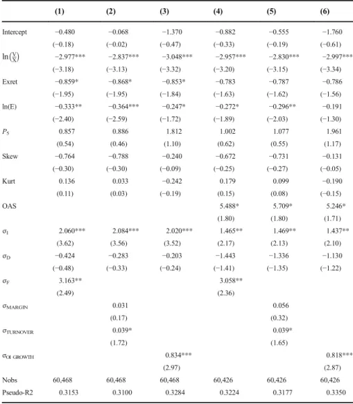
Table 3 Probability of bankruptcy: margin and turnover volatility
(1) (2) (3) (4) (5) (6) Intercept −0.480 −0.068 −1.370 −0.882 −0.555 −1.760 (−0.18) (−0.02) (−0.47) (−0.33) (−0.19) (−0.61) lnV X −2.977*** −2.837*** −3.048*** −2.957*** −2.830*** −2.997*** (−3.18) (−3.13) (−3.32) (−3.20) (−3.15) (−3.34) Exret −0.859* −0.868* −0.853* −0.783 −0.787 −0.786 (−1.95) (−1.95) (−1.84) (−1.63) (−1.62) (−1.56) ln(E) −0.333** −0.364*** −0.247* −0.272* −0.296** −0.191 (−2.40) (−2.59) (−1.72) (−1.89) (−2.03) (−1.30) P5 0.857 0.886 1.812 1.002 1.077 1.961 (0.54) (0.46) (1.10) (0.62) (0.55) (1.17) Skew −0.764 −0.788 −0.240 −0.672 −0.731 −0.131 (−0.30) (−0.30) (−0.09) (−0.25) (−0.27) (−0.05) Kurt 0.136 0.033 −0.242 0.179 0.099 −0.190 (0.11) (0.03) (−0.19) (0.15) (0.08) (−0.15) OAS 5.488* 5.709* 5.246* (1.80) (1.80) (1.71) σI 2.060*** 2.084*** 2.020*** 1.465** 1.469** 1.437** (3.62) (3.56) (3.52) (2.17) (2.13) (2.10) σD −0.424 −0.283 −0.203 −1.443 −1.336 −1.130 (−0.48) (−0.33) (−0.24) (−1.41) (−1.35) (−1.22) σF 3.163** 3.058** (2.49) (2.36) σMARGIN 0.031 0.056 (0.17) (0.32) σTURNOVER 0.039* 0.039* (1.72) (1.65) σOI GROWTH 0.834*** 0.818*** (2.97) (2.87) Nobs 60,468 60,468 60,468 60,426 60,426 60,426 Pseudo-R2 0.3153 0.3100 0.3284 0.3224 0.3177 0.3350
This table reports the coefficients from the estimation of a discrete hazard model, where the dependent variable is equal to one if the firm files for bankruptcy within the following 12 months and zero otherwise. Variable definitions are provided in AppendixI. Standard errors are clustered by firm and month
Ta b le 4 Binary recursi v e p arti tioning an alysis : p robabi lity of bankrupt cy P a nel A : P re di ctive a bili ty (1 ) (2) (3 ) Va ri a b le s ln V X ; Exre t ; ln E ðÞ ; σ ω;AI P5 Sk ew , Kurt ln V X ; Ex ret ; ln E ðÞ ; σ ω;AI P5 Sk ew , Kurt , σF , σIQ R , σFE PS , σMA RG IN , σTURNOVE R , σOI G R OW TH , σSAL E S G ROW T H ln V X ; Ex ret ; ln E ðÞ ; σ ω;AI P5 Sk ew , Kur t , σF , σIQ R , σFE PS , σMA R G IN , σTURNOVER , σOI GROW TH , σSALE S G ROW T H , OAS AUC (L ea rn ing sa m pl e) 0. 960 9 0 .95 7 2 0 .961 0 AUC (T es t sam ple ) 0. 921 5 0 .93 3 7 0 .926 0 P5 (AUC(k)-AUC(k-1)) 0.0027 − 0. 008 8 Re la tive cost 0 .171 6 0 .13 7 4 0 .139 0 Pa ne l B : V ar ia ble im p or tan ce (1) (2) (3 ) T o ta l P rim a ry S p litt ers T o ta l P rima ry Spli tters T otal Pri m ary S plitters ln V X 10 0.0 0 10 0.0 0 1 00. 00 1 00. 00 1 00. 00 10 0.0 0 Ex re t 7 9.7 3 2 0 .9 3 31. 28 0 .00 30. 26 0. 00 ln( E ) 7 1.8 5 1 4 .5 1 75. 70 0 .00 79. 17 2. 12 σ ω AI 3 8 .8 5 2 3.0 4 2. 05 0 .00 2. 33 0. 00 P5 3 5 .2 9 3 .4 9 76. 49 8 .16 78. 10 8. 15 Sk ew 3 2 .0 6 0 .0 0 26. 33 19.3 3 26. 72 1 9 .33 Kurt 9.8 7 3.3 1 28. 15 0 .00 28. 58 0. 00 OAS 94. 35 0. 00 σF 20. 48 5 .59 21. 80 5. 55 σIQ R 23. 80 5.1 1 20. 91 5. 11 σFEP S 38. 81 1 1 .2 2 2 3 .1 1 10. 98 σMAR G IN 10. 93 7 .04 12. 05 8. 44
Ta b le 4 (c o n tin ue d) σTU R N OV E R 7. 48 2 .72 7 .63 2. 76 σOI GROWTH 42. 47 4 .37 43. 90 4. 37 σSALES G ROWTH 17. 74 10 .14 17. 91 10. 14 T h is tabl e reports the resul ts of a b inary recursi ve partiti oning anal ysi s of th e o ne-year -ahead p ro babili ty of bankruptcy . W e us e the classificati on an d reg re ssi on tr ee s m eth odo log y (C AR T) (B re im an et al . 19 84 ) to cr ea te a d ec isio n tr ee tha t cla ss ifie s fi rm-y ea rs into b ank ru pt or no nba nk rup t. W e foll o w the GI NI rul e to ch oos e the o p tim al sp lit at ea ch n ode of the tr ee . B ase d on th is ap pr o ach , w e g en er ate th e m ax im al tree and a set o f sub -tr ee s. W e the n use ten fo ld cr oss v alida tion to estima te th e ar ea u n d er th e R O C cu rv e( A U C ) fo r th ed if fe re n t sub-trees and retai n the m in imal cost tr ee. P an el A re po rt s sum m ar y st atis tic s fo r the pr ed ic tive abili ty of the m odel. P5 (AUC(k)-AUC(k-1)) is th e 5 th p ercent ile of th e d if ference bet w ee n the AUC of the augm en ted m o d el re p o rt ed in col u mn k and th e AUC o f th e m o d el re po rte d in co lu mn k-1. W e use b oots tra p re sa m pli n g to cal cu lat e th is statist ic. Relative cost is th e su m of th e p er ce nta g e o f ty p e I an d typ e II er ro rs. P an el B pr esen ts the im por ta nce sc o re s for th e v ar ia b les in the m ode l. Th ese sc o re s are ca lcu lat ed as the sum of the improvement tha t ca n b e attr ibu ted to a g iv en va ri ab le at ea ch n ode o f the tre e. T o ta l v ar ia ble impo rt anc e ta k es int o ac co unt th e ro le o f the v ar ia b le as a su rr oga te , while the col umn p rimary spli tter only tak es in to ac co u n t the ro le o f the v ar ia ble as a pr ima ry split ter . The ana lys is is b ase d on a sa m pl e o f 61, 301 fi rm -m ont hs fo r th e pe ri od Ja nu ar y 199 6 thr ou gh to De ce mb er 201 2
economically important explanatory variable. Individually, the most important measure of asset volatility isσI(marginal effect of 0.0531 is the largest in the first 6 columns of Panel B of Table2).
Models (7) to (14) in Panel A combine different measures of asset volatility. We do not include σE and σIin the same specification due to multi-collinearity (Panel D of Table1 shows that σEand σI have a parametric correlation of 0.8814). In model (7), we start with issuer-level determinants (ln Vit
Xit
, Exretit, ln(Eit),P5,it, Skewit, and Kurtit)
andσE. We then add a measure of volatility from the credit markets, σD. Combining market-based measures of asset volatility from the equity and credit markets is superior to examining equity market information alone. (The pseudo-R2 marginally increases from 39.22% in model (1) to 39.84% in model (7) and from 28.52% in model (2) to 28.53% in model (11).) However, the coefficient on σD is not statistically significant when σD is combined with σI in model (11). In model (8), when we add our first
measure of fundamental volatility, σF, we find that both σD and σF are significantly associated with bankruptcy but σE is not. When σF is added to σIand σD in model (12), σI and σF are significant but σD is not. Using the interquartile range of the RNOA distribution and the dispersion of analyst forecasts as measures of fundamental volatility in models (9) and (13) and in models (10) and (14), respectively, we find similar results: combining measures of volatility from market and fundamental sources improves explanatory power of bankruptcy prediction models. While we do not run a horse-race between the fundamental volatility measures, we believe this could be an interesting avenue for future research. In an untabulated robustness analysis, we document further that our fundamental volatility measures also improve upon the explanatory power of a bankruptcy prediction model that includes Merton-based volatility and leverage measures (e.g., Bharath and Shumway 2008). This approach takes equity prices, equity volatility, and current leverage as given and then solves iteratively for asset value and asset volatility that price equity as a call option on the asset value of the firm.
In Panel C, we add a control for the spread level, OAS. We find that OAS subsumes σE and σD, which both cease to be significant in models (1) and (3). Fundamental volatility measures remain significant, both when included by themselves (models (4) to (6)) and when combined with σE, σI andσD (models (8) to (10) and (12) to (14)). Interestingly, the marginal effects reported in panel D of Table2 reveal that, after controlling for credit spreads, the difference in the relative importance of market-based and fundamental-based measures is more muted. For example, in models (12) to (14) σF, σIQR and σFEPS have similar importance to the market-based measures. The fact that σF, σIQR and σFEPS remain significant, after controlling for OAS could be consistent with the market not paying enough attention to fundamental measures of asset volatility.
In Table3, we start with a model that includesσI,σD, andσF, in column (1).6We then replaceσFby the volatility of operating profit margins,σMARGIN, and the volatility of asset turnover,σTURNOVER, in the spirit of the Dupont profitability decomposition. The Pearson (Spearman) correlation between σMARGINand σTURNOVER volatility is 0.0087 (−0.1665) (Table1Panel C). When we include bothσMARGINandσTURNOVER
6
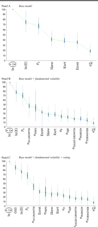
Base model
Base model + fundamental volatility
Base model + fundamental volatility + rating Panel A
Panel C Panel B
Fig. 1 Variable importance: bankruptcy prediction. Panels A, B, and C of this figure present the distribution of the variable importance scores of the models reported in Table4, columns (1), (2), and (3), respectively. We form 100 bootstrap samples and estimate the minimum cost tree for each of these samples. We report the minimum, 25th percentile, median, 75th percentile, and maximum of the variable importance scores for each variable
in equation (4), we find thatσTURNOVERis marginally significant butσMARGINis not (column (2)). We obtain similar results when we control for OAS in column (5)). The volatility of operating income growthσOI GROWTHis significant in both specifications (columns (3) and (6)). In unreported analysis, we find similar results with the volatility of sales growth,σSALES GROWTH, but due to its high correlation withσOI GROWTHwe do not report these results separately.
One limitation with the traditional discrete hazard model analysis is that it cannot capture nonlinearities and interactions that are likely among the independent variables. As an alternative methodological approach, we analyze our default data using the classifica-tion and regression trees methodology developed by Breiman et al. (1984).7Frydman et al. (1985) apply this technique to the prediction of financial distress and document that it outperforms discriminant analysis in out-of-sample tests. The data is recursively split into more homogeneous subsets, using the Gini rule to choose the optimal split at each node of the tree. Based on this approach, we generate a maximal tree and a set of sub-trees. We then use tenfold cross validation to estimate the area under the receiver operating characteristic curve (i.e., AUC) for the different sub-trees and retain the minimal cost tree. The resulting tree structure allows for nonlinear and interactive associations between probability of default and the different explanatory variables, alleviating the concern that documented results are simply due to method variance.
To focus on the relative importance of accounting- and market-based measures of asset volatility, we first apply this technique to a basic set of bankruptcy determinants, i.e., ln Vit
Xit
, Exretit, ln(Eit), P5,it, Skewit, Kurtitand a representative market-based measure of
asset volatility that combines information from implied equity option data and debt market volatility,σωAI. The CART estimation does not pose the same multicollinearity issues as the discrete hazard model estimation reported in Tables2and3, and therefore we can include all asset volatility measures simultaneously in the model. We thus augment the set of bankruptcy predictors with our seven fundamental volatility measures:σF,σIQR,σFEPS,
σMARGIN,σTURNOVER,σOI GROWTH,σSALES GROWTH.
Panel A of Table4reports summary statistics for the predictive ability of the resulting trees. Column (1) serves as the benchmark case where no fundamental-based measures of asset volatility are included. Comparing columns (1) and (2), it is clear that the test-sample (out-of-sample) AUC improves with the inclusion of fundamental-based measures of asset volatility. Note that the sample AUC for the augmented model is 0.9337, while the test-sample AUC for the basic model that only includes market volatility is 0.9215. We use bootstrap resampling to test the statistical significance of improvement in AUC. In particular, we construct 100 bootstrap samples and apply CART to each of these samples, thus building 100 different trees for each set of variables. We then compute the difference between the AUC of each of the augmented models and the AUC of the basic model. The 5th percentile of this difference is positive for the augmented model (column (2)), indicating that the improvement in the AUC achieved by incorporating the fundamental volatility measures is statistically significant at conventional levels. The relative cost (the simple sum of type I and type II classification errors) is also reduced by the inclusion of fundamental asset volatility measures. In the base model the relative cost is 0.1716.
7
We use the Salford Predictive Modeler software suit, developed by Salford Systems, to perform the CART analysis.
However, the inclusion of accounting based measures of asset volatility lowers the relative cost measure to 0.1374. The inclusion of OAS in the model (column (3)) does not significantly increase the AUC, with respect to the model that includes fundamental volatility information, and, in contrast, increases the relative cost.
To further understand the economic significance of fundamental-based measures of asset volatility, we compute importance scores for each of the variables in the model (Panel B of Table4). These scores attempt to measure how much work a variable does in a particular tree. They are calculated as the sum of the improvement that can be attributed to that variable at each node of the tree, weighted by the number of observations passing through that node (i.e., splits lower in the tree with only a smaller fraction of data passing through receive lower scores). For example, suppose that there are N observations in a given tree node (the parent node,t) and that variablesis chosen to split those N observations into two child nodes (tLandtR). Variables, together with
all the other variables used to recursively split the sample data in the tree, is called a primary splitter. The improvement attributed to variable sin that specific node t is simplyΔR(s,t) =R(t)−R(tL)−R(tH), withR tð Þ ¼N1 ∑
xn∈t
yn−y tð Þ
ð Þ2
, and effectively re-flects a change in the sum of square errors as a result of the split. To compute the variable importance score for variables, we thus (1) identify all the nodestin which variable
sis used as a splitter, (2) compute the split improvement (ΔR(s,t)) for all of these nodes, (3) adjust the split improvement to take into account the percentage of the sample flowing through each node, (4) add all the resulting improvement scores to compute the raw variable importance of variables, and (5) rank and scale all raw variable importance scores, such that the variable with highest importance receives a score of 100. Following Breiman et al. (1984), we also examine the role that each variable plays as a surrogate. A surrogate is simply a substitute for a primary splitter at a certain node. The surrogate divides the data in a similar way to the primary splitter and may thus be used to replace the primary splitter when the primary splitter is missing. Our total variable importance score considers the role of each variable both as a primary splitter and as a surrogate. It is estimated following the approach described above, except that we now identify all the nodes where CART selects the variable either as a primary splitter or a surrogate and add all the corresponding improvement scores. Leverage is the most important variable in models (1) and (3). Furthermore, the importance scores of fundamental-based measures of asset volatility are higher than those of market-based volatility measures, both considering just the role of each variable as primary splitter and its combined role as primary splitter and surrogate. When OAS is included in the model (model (3)) it becomes the second highest importance variable (after leverage). WhileOASis assigned a total variable importance score of 94.35 in model (3), it has no importance as a primary splitter. This is in contrast with leverage, which has a total variable importance of 100 and a variable importance as a primary splitter of 100. This suggests that, while OAS is not directly used in the prediction tree, it plays an important role as a surrogate, i.e., it could replace leverage and other predictors if they were missing. Most importantly, the variable importance of the fundamental volatility measures remains high when OAS is added to the model, ranging from 7.63 to 43.90, compared to the 2.34 variable importance ofσωAI.
Variable importance scores capture the role played by a variable in a specific tree, and CART trees may be sensitive to the training data. This issue is partially addressed by the fact that we use cross-validation to build test samples and choose the optimal
tree. To further circumvent this potential issue and assess the stability of our variable importance scores, we build 100 bootstrap samples and compute variable importance scores for each of these samples. Figure 1 plots the distribution (specifically, the minimum, 25th percentile, median, 75th percentile and maximum) of these scores. Note that the ranking of the variables in each of the panels of Fig.1 may not exactly correspond to the ranking of the variables in Table4, Panel B. This is because the ranking in Fig.1is based on the median importance of the variable in the 100 trees built using the bootstrap samples, whereas the importance scores reported in Table4, Panel B are based on the tree built using our original data. Both Figure 1 and Table 4 highlight the importance of fundamental asset volatility for predicting defaults out of sample, when compared to bothσωAIand the basic set of bankruptcy determinants.
3.2 Cross-sectional variation in credit spreads 3.2.1 Unconstrained analysis
Having established the information content of our candidate measures of asset volatility for bankruptcy prediction, we now turn to assess the information content of the same measures for secondary credit market prices. As discussed in section2.5, under the assumption that security prices in the secondary credit market are reasonably efficient, we expect to see that the determinants of bankruptcy prediction models should also be able to explain cross-sectional variation in credit spreads.
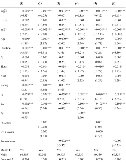
Table 5 reports estimates of equation (5). This is our unconstrained analysis of how and whether different measures of asset volatility have information content for security prices. We include month fixed effects to control for macroeconomic factors, and as such we do not report an intercept. As discussed in section 2.5, we include additional issue specific measures (Ratingit, Ageit, and Durationit) to
help control for other known determinants of credit spreads. Of course, we may be controlling for characteristics that subsume volatility by including these determi-nants, especially Ratingit. For example, the rating agencies may be using
algo-rithms to assess credit risk that span fundamental and market data sources, and as such included rating categories might subsume the ability of this data to explain cross-sectional variation in credit spreads. In unreported analysis, we find that our inferences of the combined information content of market- and accounting-based information to measure asset volatility are unaffected by the inclusion of Ratingit.
Across all models estimated in Table 5, we find expected relations for our primary determinants. Credit spreads are consistently decreasing in (i) distance to default barrier, ln Vit
Xit
, and (ii) firm size, ln(Eit). Credit spreads are
consis-tently increasing in (i) credit rating (scaled to take higher values for higher yielding issues), Ratingit, and (ii) time since issuance, Ageit. Recent excess
equity returns, Exretit, is usually negative across different models but is not
consistently significant at conventional levels. Option-adjusted duration, Durationit, is usually negatively associated with credit spreads. P5, it and Skewit
exhibit negative coefficients across most models but are often not significant at conventional levels. Conversely, Kurtit exhibits positive but often insignificant