Location of the labour force in an interregional general
equilibrium model
Morten Marott Larsen Ph.D. Student
University of Copenhagen, Institute of Economics and AKF (Institute of Local Government Studies – Denmark)
May 2002
Abstract
Interactions between regions are important when the labour market and infrastructure are considered. Labour market and infrastructure are closely related. Employment generates commuting, better infrastructure may result in more jobs, and both employment and infrastructure effects interact with the location of the labour force. To investigate these relationships an interregional general equilibrium model has been constructed. The point of departure is a search equilibrium model in which unemployment occurs because it takes time to match a vacancy with an unemployed worker (frictional unemployment). A heterogeneous labour force differs with respect to taste for leisure and taste for residence. Factors such as regional wage levels, unemployment benefits, regional taxes, the allowable tax deduction for commuting costs, consumer prices, distance, commuting costs, utility of leisure, and utility of residence, determine the equilibrium of the economy.
1. Introduction
This paper focuses on an important component of transport, commuting1. Improvement in
infrastructure and means of transport, a larger labour force, changed production structure, a more specialized labour market, changed structure of household, and district plans can be some of the reasons why the amount of commuting has increased by at least 25% from 1980 to 1995 in Denmark (Andersen (1999)).
This paper deals mainly with the economic effects of transport, whereas more traditional transport models focus on modal choice and route planning.
When evaluating an improvement in infrastructure benefits from a more integrated labour market
and costs such as emissions (CO2 or NOx) are important components. The benefits are not only
timesaving. An integrated labour market can result in more production because of agglomeration effects and lower unemployment because workers are willing to seek more jobs. The latter effect is examined in this paper.
The time horizon in the analysis is the long run. Therefore, it is important to incorporate location effects. In the model, the location of the workers is linked to the labour market choices that the workers make. When an unemployed worker gets a job he has planned whether or not to move nearer to the place of production. The choice is influenced by regional after-tax wage levels, consumer prices, after-tax commuting costs, the utility of leisure, the utility of place of residence, etc.
It is the purpose of this paper to develop a model which integrates commuting, the location of workers, and the labour market. The model should be able to quantify important effects which are due to infrastructure developments or policies concerning commuting, location of workers, and the labour market.
1 26% of an individual’s daily transport efforts measured in kilometres in Denmark in 1999 were
This paper describes a model which is intended to be applied to examples of infrastructure improvement and transport policies, such as for instance a taxation-based change in commuting costs. It is from this perspective that the paper is to be read.
The paper is organized as follows. Section 2 describes the model. Section 2.1 deals with the labour market. The firms which are producing commodities are presented in section 2.2, and section 2.3 concerns the transport sector which is transporting commuters. Section 2.4 defines the workers and section 2.4.1 describes the search and location behaviours of the workers. Section 2.5 deals with the regional wage, and a description of the public sector is in section 2.6. Finally, section 3 discusses the model and the conclusions of the paper are in section 4.
2. The model
The fundamentals of the labour market are formulated in Pissarides (2000) in which equilibrium unemployment is present because it takes time to match a vacancy and an employed worker. Munksgaard and Pilegaard (2000) developed a regional version of the model, but the location of the workers was exogenous. This was also the case in Larsen (2002) where a three region model was established to evaluate for example the consequences of a reduction in the allowable tax deduction for commuting costs. Both Munksgaard and Pilegaard (2000) and Larsen (2002) included several types of transport, but they did not include location effects. This paper focuses on commuting and location. Wasmer and Zenou (2000) also use the standard Pissarides setup when they examine how workers’ locations in an agglomeration depend on commuting costs, the price of land, and the value of job search and employment.
The model in this paper has only two regions. It is chosen to evaluate the location of the workers in this rather simple setup, before building a large scale model with a substantial interregional interaction. In principle, many regions could be added, but when adding extra regions the search and location decision of the workers become very complex as indicated later in the presentation of the workers.
The model is dynamic, but is solved in steady state only. When an experiment is carried out in the model, the new steady state is compared with the base line scenario. This allows for a comparison
of the two different equilibriums in the model. As a consequence, nothing is said about the dynamic process between the two steady states.
The following notation is used: The name of a variable is defined by one or two letters and sometimes a superscript. Subscripts are used to define the dimensions of the variable. There are two regions r0{A,B}, and normally the subscript r means regions, but sometimes it is convenient to use the subscript r as place of residence and the subscript s0{A,B} as place of work. The subscript t is
the time period. For example, , ,
M r A s B t
N = = is the number of employed workers in the sector which is
producing commodities (“M”), who live (“r”) in region A, work (“s”) in region B at time t.
The subscript i0(A,B) indicates the place of production and in this connection the subscript r
indicates place of demand. For example, M, ,
i A r B t
Y= = is the production of commodities which are
produced in region A, and consumed in region B, at time t.
2.1 The labour market
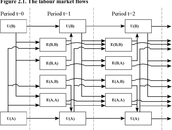
Workers make decisions about where to search for a job and where to locate, choosing between two regions. Figure 2.1 shows the labour market flows in the model.
In figure 2.1 there are two regions A and B. r0{A,B} denotes place of residence whereas s0{A,B}
denotes place of work. The people in the labour force are either unemployed workers U(r) or
employed workers E(r,s). In period t=0 an unemployed worker in region A, U(A), has to make a decision about where to search for a job and where to locate if he gets a job. There are four outcomes: 1) E(A,A). He gets a job in region A. 2) E(B,B). He gets a job in region B and moves to region B. 3) E(A,B). He gets a job in region B and becomes a commuter with residence in A. 4)
U(A). He gets no job. Once employed the worker does not search for another job, but stays in the job until sacked.
Figure 2.1. The labour market flows
There are some simplifications in the specification. There is no job search while the worker is employed. Every period workers get sacked, but the separation rate is exogenous. Unemployed workers do not move. If an unemployed worker gets a job in the region in which he lives then he does not move to another region when he gets the job. These are all assumptions which are not crucial, but are very convenient when formulating the model.
Furthermore, location in the model is focussed on location in connection with new jobs. Workers’ preferences for the regions are exogenous. Commuting between regions is present in the model because some workers decide not to move when they get a job in another region.
In the underlying search model formulated by Pissarides (2000) the search activity is costly for both firms and workers. Resources are used before job creation and production can take place. Vacant jobs and unemployed workers are matched to each other according to the matching technology in
the region. The regional matching function describes the number of jobs which are created in every period, Mr,t, as a function of job candidates, JSr,t, and vacancies/job openings JOr,t:
(
) (
)
1, , ,
r r
r t r r t r t
M =ϕ JS η JO −η (2.1)
where 0ϕr > is a scaling parameter and 0<ηr <1is the matching elasticity. The matching function is increasing in both job candidates and vacancies, concave, and homogeneous of degree one. Empirical literature supports the Cobb-Douglas specification of the matching function (Pissarides (2000)).
The vacancies and unemployed workers that are matched in a given period t are randomly selected
from the sets of job candidates and vacancies. Hence the process that changes the state of vacant jobs is Poisson with the rate Mr,t/JOr,t. By the specification of the matching function the rate at
which vacant jobs become filled, qr t, is a function only of the ratio of vacancies to job candidates:
, , / , , r
r t r t r t r r t
q ≡M JO =ϕ θ−η (2.2)
whereθr t, ≡JOr t, /JSr t, . This ratio is denoted labour market tightness. During a period a vacant job is matched to an unemployed worker with the probabilityqr t, , so the mean duration of a vacancy is1/qr t, . If labour market tightness is increasing then the mean duration of a vacancy is increasing also, as∂qr t, /∂θr t, ≤0.
Unemployed workers move into employment according to a related Poisson process with the rate
Mr,t/JSr,t and this implies that the rate is equal to qr t r t,θ , . The mean duration of unemployment is
(
, ,)
1/ qr t r tθ . Consequently, unemployed workers find jobs more easily when there are more vacancies in relation to job candidates.
2.2 The firms
In every region there is one large firm that produce commodities. Although the firm is large it is assumed that it does not make use of the market power. The firm employs many workers and it is assumed that the wage rate is given by a bargain between the regional labour union and the firm when the worker is hired. The firm considers all workers as homogeneous.
The only input is labour and it is assumed that there is a cost connected with the job openings. The production function is:
, , , M M M M M r t r t r r t r Y =N −ρ JO − f (2.3) where M, r t Y is regional production, M, r t
N is the labour input, M
r
ρ is the cost connected with job
openings, M,
r t
JO is job openings/vacancies and M
r
f is fixed cost.
Because of exogenous shocks to the firm such as changes in relative demand or technology, existing jobs become vacant every period at the exogenous separation rate sr, so it is necessary to create job
openings for replacement. The job openings are not filled at once as mentioned earlier, but vacancies and unemployed workers are matched through the matching process. The firm’s labour force changes according to:
, , , ,
M M
r t r t r t r r t
N• =q JO −s N (2.4)
where the choice variable of the firm is M, r t
JO and the separation rate is sr. In steady state there is no
growth in the firm’s labour force, so M, 0
r t N• = which implies: , , , 1 M r t r r t r t JO s N q = (2.5)
In steady state the regional job openings are equal to the number of job separations in the firm multiplied by the mean duration of a vacancy. If the mean duration of a vacancy is increasing then more job openings are needed to keep the same amount of employed workers in the firm. A larger number of employed workers in the firm also require more job openings.
The firm makes a profit in each period:
, , , , , M M M M r t p Yr t r t w Nr t r t π = − (2.6) where M, r t
p is the regional output price of the commodity and M, r t
w is the regional wage.
The discounted present value of the firm’s profit is:
, 0 v r t r e r tdt π =∞ − π
∫
(2.7)where rv is the internal interest rate of the firm. The firm maximizes the discounted present value of profit with respect to M,
r t
JO subject to equation (2.4).
The maximizing problem is solved by defining the Hamiltonian where the control variable is M,
r t
JO
and the state variable is M, r t
N . The Hamiltonian function is defined and the first order conditions are deduced:
(
) (
)
, , , , , , , , , ( M, M) r tv M M M M M M r t r t r t r t r t r t t r t r t r r t H N JO =e− p Y −w N +λ q JO −s N (2.8) , , , 0 v r t M M r t r t r t M r t H e p q JO δ ρ λ δ = − − + = (2.9)(
, ,)
, v r t M M r t r t t r v M r t H e p w s r N δ λ λ λ δ • − = − − = − + (2.10) In steady state λt 0 •= and when substituting equation (2.9) into (2.10) the following condition is
obtained after some calculation:
(
)
, , , 1 1 / M M r t v M r t r r r t p w r s ρ q = − + (2.11) The reason why the marginal product of labour does not equal the wage is the cost connected withjob openings.
(
v)
/ M,r r r t
r +s ρ q is the expected capitalized value of the firm’s costs connected with
job openings. This cost is increasing if the separation rate or the mean duration of a vacancy is increasing.
The present value of an occupied regional job at time t ,
N r t J can be written:
(
)
, , , , , 1 , 1 , 1 1 1 M r t N M M V N r t v r t M r t r r t r r t r t Y J p w s J s J r N + + ∂ = − + + − + ∂ (2.12) where V, 1 r tJ + is the value of a vacancy at time t+1. In steady state the equation simplifies to:
M M V N r r r r r v r p w s J J r s − + = + (2.13)
The present value of an occupied regional job is later used in section 2.5, when the regional wage is determined.
2.3 The transport sector
Transport of commuters is the only type of transport. When commuters are transported to and from their place of work it is defined as a transport flow. There are four transport flows (from r to r, from
s to s, from r to s, and from s to r). Every transport flow has its own transport price.
A central variable is the transport quotient C, r s
t which is assumed to incorporate all kind of conditions regarding the four transport flows in the model. These conditions are distances, the state of infrastructure, speed limits, etc. A priori it is assumed that distances inside the regions are shorter than the distances between the two regions.
The production technology in the transport sector is constant return to scale, and there is no profit. In this sector no cost is connected with hiring. The four production functions are defined:
, , , , C C C r s t r r s t Y =k N (2.14) where C r
k is a positive regional scaling parameter and C, , r s t
N is the number of workers in the transport
sector.
Profit maximization leads to regional prices of commuting:
, , M r t C r t C r w p k = (2.15)
The equilibrium condition in which supply equals demand is defined:
, , , , ,
C C r s t r s r s t
Y =t N (2.16)
where Nr,s,t are commuters from place of residence r to place of work s. All employed workers are
commuters even if the employed worker lives and works in the same region. The number of commuters is given by:
, , , , , , , , for r=s for r s M C r r t r s t s r s t M r s t N N N N + = ≠
∑
(2.17) It is assumed that workers who transport commuters are located in the place of residence of thecommuters. Furthermore, it is assumed that workers in the transport sector are also commuters within the region.
2.4 The workers
The size of the labour force is fixed. Workers are homogeneous from the firm’s point of view, but workers differ with respect to preferences for leisure and residential location. The residential and search pattern choices influence unemployment. Workers consume the commodities, leisure and place of residence. Furthermore, they are affected by the amount of commuting in the region. Commuting generates negative externalities because of emissions, noise, and accidents. Emissions such as CO2 or NOx are considered a global externality whereas noise and accidents are a local
externality. No other externalities are considered in this paper. The regional flow utility function in region r at time t is:
( )
1 1 , , , M M L L G r t r t r r t t r U C F R E E γ γ γ γ β − − ν µ = + + − − ∑
(2.18) where L rE and EGare the local and the global externality respectively, ν is the parameter of leisure,
and µ is the parameter of living in a region. Every worker is assigned a ν and a µ which are both
uniformly distributed between zero and one. Furthermore, it is assumed that ν and µ are
independent. To make this version simple it is assumed that the workers have preferences for one region only and that the utility of living in that region is R. It is assumed that no regional differences in the specification of utility of commodities are present. The elasticity of substitution between the two regional commodities γ and the scaling parameterβMis identical in both regions. This implies
that it is not necessary to consider exactly where every worker lives and will be living in future periods. However, fewer degrees of freedom are left when calibrating the data. The exogenous
amount of leisure L r F is defined: , if an employed worker if an unemployed worker E L r s r U r F F F = (2.19) where U E, E, r r r r s r
F >F >F ≠ which means that the unemployed worker has more leisure than the
employed worker who works and lives in the same region and the employed worker who commutes between the two regions has least leisure.
The local and global externalities are:
(
)
, , , , , L L M r t r r r t s r t E =ε N +N (2.20) , , , G G t r s t r s E =ε∑
N (2.21) where L rε and εGare the parameters which measure the externalities according to the numbers of
commuters in the region and the total amount of commuters, respectively. Remember, that by definition a worker who works and lives in the same region is also a commuter. Consequently, the total number of commuters equals the total number of employed workers.
The income of a person in the labour force is determined by his connection to the labour market. For an unemployed worker, income is U,
r t
I and for an employed worker E, , r s t I :
(
)
, 1 , , / , U w L F r t t r r t r t r t I =d −τ +T +π L (2.22)(
)
(
)
, , 1 , , 1 , , / , E w C C C L F r s t s r r t r s r t r t r t I =w −τ −p t −τ +T +π L (2.23) where w rτ is the regional tax rate and τCis the rate of allowable tax deduction for commuting.
,
L r t
T is
the regional lump sum transfer and , / F,
r t Lr t
π is regional profit divided by the labour force in the
region as it is assumed that every member of the labour force owns an equal share of the regional firm.
The workers maximize the flow utility in every period as there is no possibility to transfer income between periods. Workers must spend all their income on consumption. Furthermore, workers do not take externalities into consideration. The maximization problem is solved and demand functions and price indexes are deduced (see calculations of standard CES functions in for example Pedersen (1998)). The price index of commodities is:
( ) ( )
1 1 1 , T M M t r t r P = β γ p −γ −γ ∑
(2.24)and the demand functions of employed and unemployed workers are:
( )
, , , , , , M E i t r s t E M i r s t T T t t p I C P P γ γ β − = (2.25)( )
, , , , M U i t r t U M i r t T T t t p I C P P γ γ β − = (2.26) where E, , , i r s tC is the consumption of commodities from region i by employed workers living in
region r and working in region s. There are eight (2x2x2) demand functions in every period whereas there are four (2x2) demand functions concerning the unemployed workers U, ,
i r t
C .
The total demand for commodities from both regions must equal production in each region:
, , , , , , , , , , E E U M i r s t r s t i r t r t i t r s r C N + C N =Y
∑
∑
(2.27) where U, r tN are unemployed workers.
2.4.1 Expected present value of future utility
In the previous section the flow utility was defined as the utility the worker enjoys in each period. However, the single worker has different connections to the labour market and lives in different regions over time. When deciding where to search for a job and where to live, future periods must be considered. This is done using the expected present value of future utility, which includes future periods.
The expected present value of future utility at period t is equal to the flow utility which is obtained at the end of the period plus the expected utilities that are obtained in future periods. The following notation is used. V is the expected present value of future utility and superscript indicates an unemployed worker (u) or an employed worker (e) and subscripts indicate place of residence (r), place of work (s) (if not an unemployed worker), the search and location strategy (l) and period t. The search and location strategy shows in which region the worker searches for a job and in which region(s) he wants to locate. It is assumed that a person enters the labour market as an unemployed worker in the region that they want to live in. Remember, that in this simple setup, workers have preferences for the same region only. Furthermore, it is assumed that the worker always seeks a job in the region in which he lives and consequently, there are two search possibilities (search in the home region only or search in both regions). The worker who seeks a job in both regions has to decide whether to stay (S) in the region he lives in or to move (M) to the other region if he gets a job
there. It is assumed that there are three strategies only: Search in home region only (l=
{
( )
r S,}
), search in both regions, but always stay in the home region (l={
( )
r s S, ,}
), and finally, search in both regions and move to the region where one gets a job (l={
( )
r s M, ,}
).The expected present value of future utility is determined for the three strategies. An unemployed worker who does not want to change his place of residence because of high preferences for the location and who is only searching for a job in the region in which he lives because of high preferences for leisure, has the following expected present value of future utility ( U, {( ), ,}
r l r S t V = ):
(
1)
, {( ), ,} , , ,(
, , {( ), , 1})
(
1 , ,)
(
, {( ), , 1})
U U E U r t r t r t r t r t r l r S t r r l r S t r l r S t V U q V q V δ = θ = + θ = + + = + + − (2.28)where δ ≥0is the discount factor, U,
r t
U is the flow utility of an unemployed worker, and
( )
{ }
, , , , 1
E
r r l r S t
V = + is the expected present value of future utility of an employed worker in period t+1 who
lives in region r, works in region r, and has the search and location strategyl=
{
( )
r S,}
.An employed worker with the same strategy has the following expected present value of future utility:
(
1)
, , {( ), ,} , ,(
, {( ), , 1})
(
1)
(
, , {( ), , 1})
E E U E r r t r r r r l r S t r l r S t r r l r S t V U s V s V δ = = + = + + = + + − (2.29)The employed worker gets flow utility at the end of the period. The separation rate determines the possibility of staying in employment in the next period.
Substituting equation (2.29) into (2.28) and using the fact that in steady state t=t+1=t+2=... yields: ( ) { }
(
)
(
,)
, , 1 1 U U E r r r r r l r S r V U βU δ β = = + + (2.30) where r r r r q s θ β δ =+ . βr expresses the relationship between getting a job and getting sacked. If the
possibility of getting a job is increasing then it becomes relatively more important what the utility of being employed is. If the separation rate is increasing then it becomes relatively more important what the utility of being an unemployed worker is.
An unemployed worker with sufficiently low preferences for leisure and sufficiently high preferences for place of residence will search for a job in both regions, but he will not change his place of residence. In steady state, an unemployed worker who searches in both regions, but always stays in the home region, has the following expected present value of future utility:
( ) { }
(
)
(
, ,)
, , , 1 1 U U E E r r r r s r s r l r s S r s V U βU βU δ β β = = + + + + (2.31)The equation is similar to equation (2.30), but the flow utility obtained when working in the other region is incorporated. The $’s indicate the possibilities of being in the three labour market states: Unemployment, employed worker in place of residence, or employed worker commuting to the other region.
Finally, if the unemployed worker searches in both regions and moves to the region where he gets a job, then he has the following expected present value of future utility in steady state:
( ) { }
(
) (
(
)
, ,)
, , , 1 ˆ ˆ 1 1 U U U E E r r r s r r r s s s r l r s M r s V γ U γ U βU βU δ β β = = + + − + + + (2.32) where ˆ s s r r r s s s r q q β γ θ θ =+ + . There are four flow utilities weighted by the possibilities of being in
each of the four states. If the probability of getting a job in the place of residence is increasing then the flow utility of being an employed worker in the place of residence becomes relatively more important. Regarding the flow utility of being an unemployed worker, there are two effects if the probability of getting a job increases in the home region. First, the flow utility of being an unemployed worker becomes relatively less important because the worker is more likely to be in employment. Second, the flow utility of being an unemployed worker in region r becomes relatively more important compared to the flow utility of being unemployed in region s because the worker is more likely to be employed in region r.
The workers differ with respect to two facts when calculating the expected present value of future utility, the values of the two parameters ν and µ. When comparing the three strategies it is possible to find the values of ν and µ which characterize the marginal worker who is indifferent between some strategies. The three strategies are compared two at time and three marginal conditions are obtained.
If the preference for living in a region is sufficiently high the worker would always locate in that region. The choice for the unemployed worker is whether or not to search for a job in the other region. The marginal condition is independent of the value of µ. The problem is solved as follows and is determined from:
( ) { } {( ) } , , , , , U U r l r S r l r s S V = =V = ⇔
(
)
(
)
, , *1 , , 1 1 E U E r s r r r r T T r T r E U E r r s r r r r I I I P P P F F F β β ν β β + − − = − + + + (2.33) where *1 rν is the marginal value of ν where a worker is indifferent between searching in the other region or not. If *1
r
ν is increasing then more workers will also search for a job in the other region.
*1
r
ν depends positively on real income if the worker is working in the other region and depends
negatively on real unemployment benefit and real income when working in place of residence. The negative dependence on real unemployment benefit occurs since the worker is more in unemployment when searching for a job in the home region only. Furthermore, the amount of leisure also matters. For instance, if a new road is built between the two regions it could result in
more leisure for the commuting workers between the two regions. Other things equal *1
r
ν will
increase in this case.
The strategies, search in both regions and move to the region where the worker gets a job, and search in home region, are also compared to find the marginal values of ν and µ:
( ) { } {( ) } , , , , , U U r l r S r l r s M V = =V = ⇔
(
)
(
)
(
)
(
)
(
)
, , *2 , , *2 1 ˆ ˆ 1 1 ˆ [ 1 ˆ ˆ ] 1 E E s s r s r r s T T r U U s s r r T r T r s E r s E s s s r r r U s U r s r r r I I P P I I P P R F F F F β β β β β γ γ β µ β γ β β β β β γ γ ν β − + + − + + = + + − + + − + + (2.34)where µ*2andν*2are the two marginal values where a marginal worker is indifferent. It can be
shown that if the amount of leisure is equal for an unemployed worker in the two regions
( U U
r s
F =F ), and the amount of leisure is equal for an employed worker in the two regions
( E, E,
r r s s
F =F ), then µ*2depends negatively on ν*2 because it is assumed that
,
U E r r r
F >F .
Finally, the last two strategies are compared: ( ) { } {( ) } , , , , , , U U r l r s S r l r s M V = =V = ⇔
(
)
(
(
) (
)
)
, , *3 *3 , , ˆ 1 ˆ ˆ E E U U s s r s s r s T r T s r E E U U s s s r s r s r I I I I P P R F F F F β γ µ β γ β γ ν − − + = + + − + − (2.35) where µ*3 and ν*3are the two values where the marginal worker is indifferent. If the amount of
leisure in the two regions is the same ( U U
r s
F =F ), then µ*3 depends positively onν*3, because it is
assumed that , ,
E E s s r s
F >F .
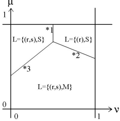
The three marginal conditions of the strategies are illustrated in figure 2.2. *1, *2, and *3 are the three marginal conditions and they refer to the three lines in equation (2.33) (*1), (2.34) (*2), and
(2.35) (*3). When ν and µ are sufficiently high l=
{
( )
r S,}
is the optimal strategy. If ν is sufficientlylow and µ sufficiently high then l=
{
( )
r s S, ,}
is the optimal strategy. Finally, when the preference for location is sufficiently low (µ is low) then the optimal strategy isl={
( )
r s M, ,}
.As noted above *1 is independent of µ and therefore *1 is vertical in figure 2.2. With the assumption that the amount of leisure is equal for an unemployed worker in the two regions and the amount of leisure is equal for an employed worker in the two regions, *2 has a negative slope and *3 a positive slope. The interpretation of a negative slope of *2 is that given µ leisure becomes more and more important as < increases and when the worker searches for job in one region only he is more often an unemployed worker with more leisure. *3 has a positive slope because it is time- consuming to commute to the other region.
Figure 2.2. The location and search behaviours of the workers
The intersection between *2 and ν=1 is above zero when the real after-tax income conditions such as wages, lump sum transfers, and profit, are generally higher in region s compared to region r. The
intersection between *3 and ν=0 is affected by the same real after-tax income conditions, but
furthermore, higher commuting costs contribute to an intersection above µ=0. Remember that a
fourth strategy: search in region s only is not included in this paper.
When the three marginal conditions are determined it is possible to calculate the number of workers using each of the three strategies. The area in figure 2.2, where l=
{
( )
r S,}
is the optimal strategy, forms a trapezium. When calculating the size of the trapezium the size of the labour force whichuses l=
{
( )
r S,}
is obtained. The same procedure applies to the strategyl={
( )
r s S, ,}
. The size of the labour force using the strategy l={
( )
r s M, ,}
can be fixed residually.In the following section it is very convenient to characterize the worker together with a search strategy. Therefore an extra subscript is added. The changed notation implies:
, , , , , M L r s t r s l t l N =
∑
N (2.36) where , , , L r s l tN are employed workers who live in region r, produce commodities in region s, have the search strategy l, at time t.
The following equilibrium conditions apply to the three strategies:
( ) { } {( ) } *{( ) } , , , , , , , , , , , L U F C r s t r r l r S t r l r S t l r S r s N = +N = =α= L − N
∑
(2.37) ( ) { } {( ) } {( ) } *{( ) } , , , , , , , , , , , , , , , , , , , L L U F C r s t r r l r s S t r s l r s S t r l r s S t l r s S r s N = +N = +N = =α= L − N ∑
(2.38) ( ) { } {( ) } {( ) } {( ) } *{( ) } , , , , , , , , , , , , , , , , , , , , , , , L L U U F C r s t r r l r s M t s s l r s M t r l r s M t s l r s M t l r s M r s N = +N = +N = +N = =α= L − N ∑
(2.39) The * lα ’s are the calculated areas of figure 2.2 and by definition are 0 * 1
l α ≤ ≤ and * 1 l l α =
∑
. The * lα ’s divide the labour force LFminus the employed workers who are transporting commuters
into the three possible strategies. On the left side of the equations are the possible states of the strategies. The relationships between the possible states of employed and unemployed workers are presented in the following. If the search strategy is l=
{
( )
r S,}
or l ={
( )
r s S, ,}
then the change in employment is the unemployed workers who get a job minus the employed workers who get sacked: ( ) { } , , {( ) } {( ) } , , , , , , , , , , , , , , L U L s t s t s r s l r s M t r l r s M t r s l r s M t N ≠ =θ q N ≠ −s N ≠ (2.40) In steady state L, , {( ), , }, 0 r s l r s M t N ≠ = which implies: ( ) { } , , {( ) } , , , , , , , , , s t s t L U r s l r s M t r l r s M t s q N N s θ ≠ = ≠ (2.41)If the search strategy is l=
{
( )
r s M, ,}
then the corresponding flow equation is: ( ) { } , , {( ) } , , {( ) } {( ) } , , , , , , , , , , , , , , , , , , L U U L r t r t r t r t r r r l r s M t r l r s M t s l r s M t r r l r s M t N = =θ q N = +θ q N = −s N = (2.42)When applying the steady state condition that the change in employment is zero, the following two equations must hold:
( ) { } {( ) } {( ) } , , , , , , , , , , , , , , , , , U U r t r t r l r s M t r t r t s l r s M t L r r l r s M t r q N q N N s θ = θ = = + = (2.43)
By substitution the two equations can be written as one equation that describes the relationship between the sizes of the two kinds of employment which are possible with the strategyl=
{
( )
r s M, ,}
: ( ) { } ( ) { } , , , , , , , , , , , , , , L r r l r s M t r t r t s L s t s t r s s l r s M t N q s N q s θ θ = = = (2.44)The intuition of the equation is clear. If the possibility of getting a job in one of the regions is increasing then the region gets relatively more employed workers compared to the other region. When the separation rate in one of the regions is increasing then the region gets relatively fewer employed workers.
If the search strategy is l=
{
( )
r s M, ,}
then the unemployed workers can be described: ( ) { } {( ) } , , {( ) } , , {( ) } , , , , , , , , , , , , , , , , , U L U U r r t r t s t s t r l r s M t r r l r s M t r l r s M t r l r s M t N = =s N = −θ q N = −θ q N = (2.45)In steady state the growth in unemployed workers is zero which implies: ( ) { } {( ) } , , , , , , , , , , , , , U r L r l r s M t r r l r s M t r t r t s t s t s N N q q θ θ = = + = (2.46)
This was the last equation that describes how workers search for a job and how employment and unemployment are related. In the next section a component regarding the choice of strategy is determined.
2.5 Wage formation
The regional wage is determined by a negotiation between the regional labour union and the regional firm which is producing commodities. The labour union is represented by a member who is searching for a job in the place of residence only, and the member has a parameter of leisure at
<=0.5. It is assumed that the negotiation can be described by a Nash bargaining process in which the benefit of a match is negotiated. The wage derived from the Nash bargaining is the wage that maximizes the weighted product of the worker’s and the firm’s net return from the job:
( ) { } {( ) }
(
)
(
)
1 , , , , , E U N V r r r r l r S r l r S r MAX NP V V J J w ω −ω = = = − − (2.47) where ω is the parameter of bargaining strength. It is assumed that value of a vacancy is equal tozero ( V 0
r
J = ). The maximization problem has the solution:
(
)
,(
,)
1 1 1 1 2 1 C M M C C U E T r r r r r r r r W r r r W r r s q w ωp ω d p t τ F F P δ θ τ τ − + + = + − + + − − − (2.48)In the solution the value of commuting cost inside the region is present. Increasing commuting costs would result in a wage demand from the labour union. Also, the value of leisure is represented. If the overall price index is increasing this would also result in a wage demand.
2.6 The public sector
The duties of the public sector are to decide the size of regional taxes and allowable tax deductions for commuting, collect taxes on wage, pay unemployment benefit, and make lump sum transfers. The income of the public sector is:
(
, , ,)
I W M M W U
t r r t r t r t r t r
G =
∑
τ w N +τ d N (2.49)i.e. the tax income from both wages and unemployment benefit in the two regions. The size of unemployment benefit is determined at national level and is linked to the wage level:
( )
, ,
ˆ M 1 ˆ M
t r t s t
d = ∂w + − ∂ w (2.50)
where 0≤ ∂ ≤ˆ 1 is an exogenous parameter. Public expenditure is:
, , , , , E U C C C M t t r t r t r s r s t r s G = d N + p t τ N
∑
∑
(2.51)i.e. the expenditure on unemployment benefit and allowable tax deductions for commuting in the two regions. The balance of the public sector is maintained:
( )
, , ˆ 1 ˆ I E L L t t r t s t G −G =λT + −λ T (2.52)3 Model discussion
The model is developed in the spirit of: “Small is beautiful”, and the model deals with the location of the labour force which is an important development compared to Munksgaard and Pilegaard (2000) and Larsen (2002). It could be argued that the model still lacks a crucial element in the location of workers, namely house prices. In the model the utility of living in a region is exogenous for the single worker and no house prices enter the model. The housing market could be implemented in the model. For example, housing could be considered a new local commodity produced by a new sector which uses labour as input. Other approaches could also be considered. In this paper, it is assumed that the firms do not use their market power. It is not an essential element in model development, and the monopolistic competition model could be applied. The fundamental question is what kind of competition describes reality most closely. This question will be left open.
The transport of commuters is simple compared to a traditional transport model. Transport effects related to modal choice and route planning could enter the model through the exogenous transport quotient. Therefore, the modelling exercise of this paper does not exclude a traditional transport model approach. When economic matters, modal choice, and route planning are important, both types of approaches should be involved. Co-operation could be developed, so that the output of the economic model could enter the traditional modal choice and route planning model which could deliver a new output to the economic model, and so on.
Also more externalities could matter. Congestion is a possible extension and also polluting firms could be included. This paper describes the fundamentals of the modelling process, and the
externalities are not crucial in that sense. But when evaluating infrastructure improvements
important costs and benefits have to be considered. In this paper emissions, noise, and accidents are included, but further research needs to be done.
Preferences for location and leisure are assumed to be uniformly distributed. This is not essential when the aim is to identify economic relations. But when quantifying the results of an experiment
the distribution of preferences does matter. However, it must be possible to reveal the preferences for location and leisure, but this is a research project in itself.
4 Conclusion
A model which integrates commuting, the location of workers, and the labour market has been constructed. It has been shown how regional wage levels, unemployment benefits, regional taxes, allowable tax deductions for commuting, consumer prices, distance, commuting costs, utility of leisure, and utility of residence, all interact when an experiment is carried out.
References
Andersen, Anne K. (2000). Commuting Areas in Denmark. AKF Forlaget, Copenhagen.
Andersen, Anne K. (1999). Location and Commuting. PhD thesis - red series, nr. 57, University of Copenhagen.
Bröcker, Johannes (1998 I). Operational Spatial Computable General Equilibrium Modelling. Ann. Rg. Sci. 32:367-387.
Caspersen, Søren, Lars Eriksen and Morten M. Larsen (2000). The BROBISSE model - a spatial general equilibrium model to evaluate the Great Belt link in Denmark. SØM publication nr. 35. AKF Forlaget, Copenhagen.
Fujita, Masahisa, Paul Krugman and Anthony J. Venables (1999). The Spatial Economy – Cities, Regions, and International Trade. The MIT Press, England.
Isard, Walther, Iwan J. Azis, Matthew P. Drennan, Ronald E. Miller, Sidney Saltsman og Erik Thorbecke (1998). Methods of Interregional and Regional Analysis. Ashgate Publishing Limited. Krugman, Paul R. (1990). Rethinking International Trade. The MIT Press.
Larsen, Morten Marott (2002). Transport economics in an applied interregional general equilibrium model. SØM publication nr. 49. AKF Forlaget, Copenhagen.
Liebing, Christian S. and Mikkel B. Munksgaard (1998). Arbejdsmarkedspolitik i en søgeteoretisk CGE-model. Masters thesis, Institute of Economics, Copenhagen University, 8/9-1998.
Madsen, Bjarne, Chris Jensen-Butler and Poul Uffe Dam (2001). A Social Accounting Matrix for Danish Municipalities (SAM-K). AKF Forlaget, Copenhagen.
Munksgaard, Mikkel B. and Ninette Pilegaard (2000). Team-modellen – Dokumentation. Working paper, Unpublished, Copenhagen.
Pedersen, Lars H. (1998). Egenskaber ved specificerede funktioner Cobb Douglas, CES og nested CES. Education note, 2. edition, Institute of Economics, University of Copenhagen.
Pissarides, Christopher A. (2000). Equilibrium Unemployment Theory. 2. edition. Massachusetts Institute of Technology.
Shoven J.B. and J. Whalley (1992). Applying General Equilibrium. Cambridge University Press. Wasmer Etienne and Yves Zenou (2000). Space, Search and Efficiency. IZA Discussion Paper No. 181. Bonn, Germany.