Unsupervised Learning Methods for Source
Separation in Monaural Music Signals
Tuomas Virtanen
Institute of Signal Processing, Tampere University of Technology, Korkeakoulunkatu 1, 33720 Tampere, Finland
9.1 Introduction
Computational analysis of polyphonic musical audio is a challenging problem. When several instruments are played simultaneously, their acoustic signals mix, and estimation of an individual instrument is disturbed by the other co-occurring sounds. The analysis task would become much easier if there was a way to separate the signals of different instruments from each other. Tech-niques that implement this are said to performsound source separation. The separation would not be needed if a multi-track studio recording was available where the signal of each instrument is on its own channel. Also, recordings done with microphone arrays would allow more efficient separation based on the spatial location of each source. However, multi-channel recordings are usu-ally not available; rather, music is distributed in stereo format. This chapter discusses sound source separation in monaural music signals, a term which refers to a one-channel signal obtained by recording with a single microphone or by mixing down several channels.
There are many signal processing tasks where sound source separation could be utilized, but the performance of the existing algorithms is still quite limited compared to the human auditory system, for example. Human listeners are able to perceive individual sources in complex mixtures with ease, and several separation algorithms have been proposed that are based on modelling the source segregation ability in humans (see Chapter 10 in this volume).
Recently, the separation problem has been addressed from a completely different point of view. The termunsupervised learning is used here to char-acterize algorithms which try to separate and learn the structure of sources in mixed data based on information-theoretical principles, such as statisti-cal independence between sources, instead of sophisticated modelling of the source characteristics or human auditory perception. Algorithms discussed in this chapter are independent component analysis (ICA), sparse coding, and non-negative matrix factorization (NMF), which have been recently used in
source separation tasks in several application areas. When used for monau-ral audio source separation, these algorithms usually factor the spectrogram or other short-time representation of the input signal into elementary com-ponents, which are then clustered into sound sources and further analysed to obtain musically important information. Although the motivation of unsuper-vised learning algorithms is not in the human auditory perception, there are similarities between them. For example, all the unsupervised learning meth-ods discussed here are based on reducing redundancy in data, and it has been found that redundancy reduction takes place in the auditory pathway, too [85]. The focus of this chapter is on unsupervised learning algorithms which have proven to produce applicable separation results in the case of music signals. There are some other machine learning algorithms which aim at sep-arating speech signals based on pattern recognition techniques, for example [554].
All the algorithms mentioned above (ICA, sparse coding, and NMF) can be formulated using a linear signal model which is explained in Section 9.2. Different data representations are discussed in Section 9.2.2. The estimation criteria and algorithms are discussed in Sections 9.3, 9.4, and 9.5. Methods for obtaining and utilizing prior information are presented in Section 9.6. Once the spectrogram is factored into components, these can be clustered into sound sources or further analysed to obtain musical information. The post-processing methods are discussed in Section 9.7. Systems extended from the linear model are discussed in Section 9.8.
9.2 Signal Model
When several sound sources are present simultaneously, the acoustic wave-forms of the individual sources add linearly. Sound source separation is defined as the task of recovering each source signal from the acoustic mixture. A com-plication is that there is no unique definition for a sound source. One possi-bility is to consider each vibrating physical entity, for example each musical instrument, as a sound source. Another option is to define this according to what humans tend to perceive as a single source. For example, if a violin, sec-tion plays in unison, the violins are perceived as a single source, and usually there is no need to separate the signals played by each violin. In Chapter 10, these two alternatives are referred to as physical source and perceptual source, respectively (see p. 302). Here we do not specifically commit ourselves to either of these. The type of the separated sources is determined by the properties of the algorithm used, and this can be partly affected by the designer accord-ing to the application at hand. In music transcription, for example, all the equal-pitched notes of an instrument can be considered as a single source.
Many unsupervised learning algorithms, for example standard ICA, require that the number of sensors be larger or equal to the number of sources. In multi-channel sound separation, this means that there should be at least as
many microphones as there are sources. However, automatic transcription of music usually aims at finding the notes in monaural (or stereo) signals, for which basic ICA methods cannot be used directly. By using a suitable signal representation, the methods become applicable with one-channel data.
The most common representation of monaural signals is based on short-time signal processing, in which the input signal is divided into (possibly over-lapping) frames. Frame sizes between 20 and 100 ms are typical in systems designed to separate musical signals. Some systems operate directly on time-domain signals and some others take a frequency transform, for example the discrete Fourier transform (DFT) of each frame. The theory and general discussion of time-frequency representations is presented in Chapter 2.
9.2.1 Basis Functions and Gains
The representation of the input signal within each framet= 1. . . T is denoted by an observation vectorxt. The methods presented in this chapter modelxt as a weighted sum of basis functionsbn,n= 1. . . N, so that the signal model can be written as xt≈ N n=1 gn,tbn, t= 1, . . . , T, (9.1) where N ≪ T is the number of basis functions, and gn,t is the amount of contribution, or gain, of thenthbasis function in thetthframe. Some methods
estimate both the basis functions and the time-varying gains from a mixed input signal, whereas others use pre-trained basis functions or some prior information about the gains.
The term component refers to one basis function together with its time-varying gain. Each sound source is modelled as a sum of one or more compo-nents, so that the model for sourcemin frametis written as
ym,t=
n∈Sm
gn,tbn, (9.2)
whereSmis the set of components within sourcem. The sets are disjoint, i.e., each component belongs to only one source.
In (9.1) approximation is used, since the model is not necessarily noise-free. The model can also be written with a residual termrt as
xt= N
n=1
gn,tbn+rt, t= 1, . . . , T. (9.3) By assuming some probability distribution for the residual and a prior distri-bution for other parameters, a probabilistic framework for the estimation of
residual term is preferred for its simplicity. ForT frames, the model (9.1) can be written in matrix form as
X≈BG, (9.4)
where X=
x1,x2, . . . ,xT is the observation matrix, B =b1,b2, . . . ,bN is themixing matrix, and [G]n,t=gn,t is thegain matrix. The notation [G]n,t is used to denote the (n, t)th entry of matrix G. The term mixing matrix is
typically used in ICA, and here we follow this convention.
The estimation algorithms can be used with several data representations. Often the absolute values of the DFT are used; this is referred to as the mag-nitude spectrum in the following. In this case, xtis the magnitude spectrum within frame t, and each component n has a fixed magnitude spectrum bn with a time-varying gaingn,t. The observation matrix consisting of framewise magnitude spectra is here called amagnitude spectrogram. Other representa-tions are discussed in Section 9.2.2.
The model (9.1) is flexible in the sense that it is suitable for represent-ing both harmonic and percussive sounds. It has been successfully used in the transcription of drum patterns [188], [505] (see Chapter 5), in the pitch estimation of speech signals [579], and in the analysis of polyphonic music signals [73], [600], [403], [650], [634], [648], [43], [5].
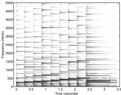
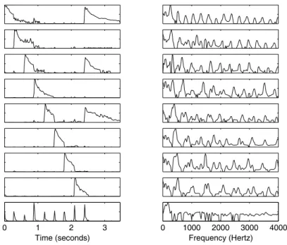
Figure 9.1 shows an example signal which consists of a diatonic scale and a C major chord played by an acoustic guitar. The signal was separated into components using the NMF algorithm described in [600], and the resulting components are depicted in Fig. 9.2. Each component corresponds roughly to one fundamental frequency: the basis functions are approximately harmonic and the time-varying gains follow the amplitude envelopes of the notes. The separation is not perfect because of estimation inaccuracies. For example, in some cases the gain of a decaying note drops to zero when a new note begins. Factorization of the spectrogram into components with a fixed spectrum and a time-varying gain has been adopted as a part of the MPEG-7 pattern recognition framework [72], where the basis functions and the gains are used as features for classification. Kim et al. [341] compared these to mel-frequency cepstral coefficients which are commonly used features in the classification of audio signals. In this study, mel-frequency cepstral coefficients performed bet-ter in the recognition of sound effects and speech than features based on ICA or NMF. However, final conclusions about the applicability of these methods to sound source recognition have yet to be made. The spectral basis decompo-sition specified in MPEG-7 models the summation of components on a decibel scale, which makes it unlikely that the separated components correspond to physical sound objects.
9.2.2 Data Representation
The model (9.1) presented in the previous section can be used with time-domain or frequency-time-domain observations and basis functions. Time-time-domain
Time (seconds) Frequency (Hertz) 0 0.5 1 1.5 2 2.5 3 3.5 0 500 1000 1500 2000 2500 3000 3500 4000 4500 5000
Fig. 9.1. Spectrogram of an example signal which consist of a diatonic scale from C5 to C6, followed by a C major chord (simultaneous notes C5, E4, and G5), played by an acoustic guitar. The notes are not damped, meaning that consecutive notes overlap.
observation vectorxtis the signal within frametdirectly, whereas a frequency-domain observation vector is obtained by applying a chosen transformation to this. The representation of the signal and the basis functions have to be the same. ICA and sparse coding allow the use of any short-time signal represen-tation, whereas for NMF, only a frequency-domain representation is appro-priate. Naturally, the representation has a significant effect on performance. The advantages and disadvantages of different representations are considered in this section. For a more extensive discussion, see Casey [70] or Smaragdis [598].
Time-Domain Representation
Time-domain representations are straightforward to compute, and all the in-formation is preserved when an input signal is segmented into frames and win-dowed. However, time-domain basis functions are problematic in the sense that a single basis function alone cannot represent a meaningful sound source: the phase of the signal within each frame varies depending on the frame position. In the case of a short-duration percussive source, for example, a separate basis function is needed for every possible position of the sound event within the
0 1 2 3 Time (seconds)
0 1000 2000 3000 4000 Frequency (Hertz)
Fig. 9.2.Components estimated from the example signal in Fig. 9.1. Basis functions are plotted on the right and the corresponding time-varying gains on the left. Each component except the bottom one corresponds to an individual pitch value and the gains follow roughly the amplitude envelope of each note. The bottom component models the attack transients of the notes. The components were estimated using the NMF algorithm [400], [600] and the divergence objective (explained in Section 9.5).
frame. A shift-invariant model which is later discussed in Section 9.8 is one possible method of overcoming this limitation [43].
The time-domain signals of real-world sound sources are generally not identical at different occurrences since the phases behave very irregularly. For example, the overtones of a pitched musical instrument are not necessarily phase-locked, so that the time-domain waveform varies over time. Therefore, one has to use multiple components to represent even a single note of a pitched instrument. In the case of percussive sound sources, this phenomenon is even clearer: the time-domain waveforms vary a lot at different occurrences.
The larger the number of the components, the more uncertain is their estimation and further analysis, and the more observations are needed. If the sound event represented by a component occurs only once in the input signal, separating it from co-occurring sources is difficult since there is no information about the component elsewhere in the signal. Also, clustering the components into sources becomes more difficult when there are many of them for each source.
Separation algorithms which operate on time-domain signals have been proposed for example by Dubnov [157], Jang and Lee [314], and Blumensath and Davies [43]. Abdallah and Plumbley [3], [2] found that the independent components analysed from time-domain music and speech signals were similar to a wavelet or short-time DFT basis. They trained the basis functions using several days of radio output from BBC Radio 3 and 4 stations.
Frequency-Domain Representation
When using a frequency transform such as the DFT, the phases of the complex-valued transform can be discarded by considering only the mag-nitude or power spectrum. Even though some information is lost, this also eliminates the phase-related problems of time-domain representations. Unlike time-domain basis functions, many real-world sounds can be rather well ap-proximated with a fixed magnitude spectrum and a time-varying gain, as seen in Figs. 9.1 and 9.2, for example. Sustained instruments in particular tend to have a stationary spectrum after the attack transient.
In most systems aimed at the separation of sound sources, DFT and a fixed window size is applied, but the estimation algorithms allow the use of any time-frequency representation. For example, a logarithmic spacing of frequency bins has been used [58], which is perceptually and musically more plausible than a constant spectral resolution.
The linear summation of time-domain signals does not imply the linear summation of their magnitude or power spectra, since phases of the source signals affect the result. When two signals sum in the time domain, their complex-valued DFTs sum linearly, X(k) = Y1(k) +Y2(k), but this equality
does not apply for the magnitude or power spectra. However, provided that the phases ofY1(k) andY2(k) are uniformly distributed and independent of
each other, we can write
E{|X(k)|2
}=|Y1(k)|2+|Y2(k)|2, (9.5)
where E{·} denotes expectation. This means that in the expectation sense, we can approximate time-domain summation in the power spectral domain, a result which holds for more than two sources as well. Even though magnitude spectrogram representation has been widely used and it often produces good results, it does not have similar theoretical justification. Since the summation is not exact, use of phaseless basis functions causes an additional source of error. Also, a phase generation method has to be implemented if the sources are to be synthesized separately. These are discussed in Section 9.7.3.
The human auditory system has a large dynamic range: the difference between the threshold of hearing and the threshold of pain is approximately 100 dB [550]. Unsupervised learning algorithms tend to be more sensitive to high-energy observations. If sources are estimated from the power spectrum, some methods fail to separate low-energy sources even though they would be
perceptually and musically meaningful. This problem has been noticed, e.g., by FitzGerald in the case of percussive source separation [186, pp. 93–100]. To overcome the problem, he used an algorithm which processed separately high-frequency bands which contain low-energy sources, such as hi-hats and cymbals [187]. Vincent and Rodet [648] addressed the same problem. They proposed a model in which the noise was additive in the log-spectral domain. The numerical range of a logarithmic spectrum is compressed, which increases the sensitivity to low-energy sources. Additive noise in the log-spectral domain corresponds to multiplicative noise in power spectral domain, which was also assumed in the system proposed by Abdallah and Plumbley [5]. Virtanen proposed the use of perceptually motivated weights [651]. He used a weighted cost function in which the observations were weighted so that the quantitative significance of the signal within each critical band was equal to its contribution to the total loudness.
9.3 Independent Component Analysis
ICA has been successfully used in several ‘blind’ source separation tasks, where very little or no prior information is available about the source signals. One of its original target applications was multi-channel sound source separation, but it has also had several other uses. ICA attempts to separate sources by identifying latent signals that are maximally independent. In practice, this usually leads to the separation of meaningful sound sources.
Mathematically, statistical independence is defined in terms of probabil-ity densities: random variables x and y are said to be independent if their joint probability distribution function1
p(x, y) is a product of the marginal
distribution functions,p(x, y) =p(x)p(y).
The dependence between two variables can be measured in several ways. Mutual information is a measure of the information that given random vari-ables have on some other random varivari-ables [304]. The dependence is also closely related to the Gaussianity of the distribution of the variables. Accord-ing to the central limit theorem, the distribution of the sum of independent variables is more Gaussian than their original distributions, under certain con-ditions. Therefore, some ICA algorithms aim at separating output variables whose distributions are as far from Gaussian as possible.
The signal model in ICA is linear: K observed variables x1, . . . , xK are modelled as linear combinations ofN source variablesg1, . . . , gN. In a vector-matrix form, this can be written as
x=Bg, (9.6)
where x =
x1, . . . xKT is an observation vector, [B]k,n =bk,n is a mixing matrix, andg=
g1, . . . , gNTis a source vector. BothBandgare unknown. 1
The standard ICA requires that the number of observed variablesK (the number of sensors) be equal to the number of sourcesN. In practice, the num-ber of sensors can also be larger than the numnum-ber of sources, because the vari-ables are typically decorrelated using principal component analysis (PCA; see Chapter 2), and if the desired number of sources is less than the number of variables, only the principal components corresponding to the largest eigen-values are selected.
As another pre-processing step, the observed variables are usually centred by subtracting the mean and their variance is normalized to the unity. The centred and whitened data observation vectorxis obtained from the original observation vector ˜xby
x=V(˜x−µ), (9.7)
whereµis the empirical mean of the observation vector, andVis a whitening
matrix, which is often obtained from the eigenvalue decomposition of the empirical covariance matrix of the observations [304]. The empirical mean and covariance matrix are explained in Chapter 2.
To simplify the notation, it is assumed that the dataxin (9.6) is already centred and decorrelated, so that K = N. The core ICA algorithm carries out the estimation of an unmixing matrix W ≈ B−1, assuming that B is
invertible. Independent components are obtained by multiplying the whitened observations by the estimate of the unmixing matrix, to result in the source vector estimate ˆg:
ˆ
g=Wx. (9.8)
The matrixWis estimated so that the output variables, i.e., the elements of ˆg, become maximally independent. There are several criteria and algo-rithms for achieving this. The criteria, such as non-Gaussianity and mutual information, are usually measured using high-order cumulants such as kurto-sis, or expectations of other non-quadratic functions [304]. ICA can be also viewed as an extension of PCA. The basic PCA decorrelates variables so that they are independent up to second-order statistics. It can be shown that if the variables are uncorrelated after taking a suitable non-linear function, the higher-order statistics of the original variables are independent, too. Thus, ICA can be viewed as a non-linear decorrelation method.
Compared with the previously presented linear model (9.3), the standard ICA model (9.6) is exact, i.e., it does not contain the residual term. Some special techniques can be used in the case of the noisy signal model (9.3), but often noise is just considered as an additional source variable. Because of the dimension reduction with PCA, Bg gives an exact model for the PCA-transformed observations but not necessarily for the original ones.
There are several ICA algorithms, and some implementations are freely available, such as FastICA [302], [182] and JADE [65]. Computationally quite efficient separation algorithms can be implemented based on FastICA, for example.
9.3.1 Independent Subspace Analysis
The idea of independent subspace analysis (ISA) was originally proposed by Hyv¨arinen and Hoyer [303]. It combines the multidimensional ICA with in-variant feature extraction, which are shortly explained later in this section. After the work of Casey and Westner [73], the term ISA has been commonly used to denote techniques which apply ICA to factor the spectrogram of a monaural audio signal to separate sound sources. ISA provides a theoretical framework for the whole separation procedure described in this chapter, in-cluding spectrogram representation, decomposition by ICA, and clustering. Some authors use the term ISA also to refer to methods where some other algorithm than ICA is used for the factorization [648].
The general ISA procedure consists of the following steps:
1. Calculate the magnitude spectrogram ˜X (or some other representation) of the input signal.
2. Apply PCA2 on the matrix ˜X of size (K
×T) to estimate the number of components N and to obtain whitening and dewhitening matricesV
andV+, respectively. A centred, decorrelated, and dimensionally reduced
observation matrixX of size (N ×T) is obtained asX =V( ˜X−µ1T),
where1is a all-ones vector of lengthT.
3. Apply ICA to estimate an unmixing matrixW.BandGare obtained as
B=W−1 andG=WX.
4. Invert the decorrelation operation in Step 2 in order to get the mixing matrix ˜B=V+B and source matrix ˜G=G+WV
µ1T for the original
observations ˜X.
5. Cluster the projected components to sources (see Section 9.7.1).
The above steps are explained in more detail below. Depending on the appli-cation, not all of them may be necessary. For example, prior information can be used to set the number of components in Step 2.
The basic ICA is not directly suitable for the separation of one-channel signals, since the number of sensors has to be larger than or equal to the number of sources. Short-time signal processing can be used in an attempt to overcome this limitation. Taking a frequency transform such as DFT, each frequency bin can be considered as a sensor which produces an observation in each frame. With the standard linear ICA model (9.6), the signal is modelled as a sum of components, each of which has a static spectrum (or some other basis function) and a time-varying gain.
The spectrogram factorization has its motivation in invariant feature ex-traction, which is a technique proposed by Kohonen [356]. The short-time spectrum can be viewed as a set of features calculated from the input signal. As discussed in Section 9.2.2, it is often desirable to have shift-invariant basis
2
Singular value decomposition can also be used to estimate the number of com-ponents [73].
functions, such as the magnitude or power spectrum [356], [303]. Multidimen-sional ICA (explained below) is used to separate phase-invariant features into invariant feature subspaces, where each source is modelled as the sum of one or more components [303].
Multidimensional ICA [64] is based on the same linear generative model (9.6) as ICA, but the components are not assumed to be mutually indepen-dent. Instead, it is assumed that the components can be divided into disjoint sets, so that the components within each set may be dependent on each other, while dependencies between sets are not allowed. One approach to estimat-ing multidimensional independent components is to first apply standard ICA to estimate the components, and then group them into sets by measuring dependencies between them.3
ICA algorithms aim at maximizing the independence of the elements of the source vector ˆg=Wx. In ISA, the elements correspond to the time-varying gains of each component. However, the objective can also be the independence of the spectra of components, since the roles of the mixing matrix and gain matrix can be swapped by X = BG ⇔ XT = GTBT. The independence of both the time-varying gains and basis functions can be obtained by using the spatiotemporal ICA algorithm [612]. There are no exhaustive studies re-garding different independence criteria in monaural audio source separation. Smaragdis argued that in the separation of complex sources, the criterion of independent time-varying gains is better, because of the absence of consis-tent spectral characteristics [598]. FitzGerald reported that the spatiotempo-ral ICA did not produce significantly better results than normal ICA, which assumes the independence of gains or spectra [186].
The number of frequency channels is usually larger than the number of components to be estimated with ICA. PCA or singular value decomposition (SVD) of the spectrogram can be used to estimate the number of components automatically. SVD decomposes the spectrogram into a sum of components with a fixed spectrum and time-varying gain, so that the spectra and gains of different components are orthogonal, whereas PCA results in the orthogonality of either the spectra or the gains. The components with the largest singular values are chosen so that the sum of their singular values is larger than or equal to a pre-defined threshold 0< θ≤1 [73].
ISA has been used for general audio separation by Casey and Westner [73], for the analysis of musical trills by Brown and Smaragdis [58], and for per-cussion transcription by FitzGerald et al. [187], to mention some examples.
9.3.2 Non-Negativity Restrictions
When magnitude or power spectrograms are used, the basis functions are magnitude or power spectra which are non-negative by definition. Therefore,
3
ICA aims at maximizing the independence of the output variables, but it cannot guarantee their complete independence, as this depends also on the input signal.
it can be advantageous to restrict the basis functions to be entry-wise non-negative. Also, it may be useful not to allow negative gains, but to constrain the components to be purely additive. Standard ICA is problematic in the sense that it does not enable these constraints. In practice, ICA algorithms also produce negative values for the basis functions and gains, and often there is no physical interpretation for such components.
ICA with non-negativity restrictions has been studied for example by Plumbley and Oja [526], and the topic is currently under active research. Existing non-negative ICA algorithms can enforce non-negativity for the gain matrix but not for the mixing matrix. They also assume that the probability distribution of the source variables gn is non-zero all the way down to zero, i.e., the probabilitygn< δis non-zero for anyδ >0. The algorithms are based on a noise-free mixing model and in our experiments with audio spectrograms, they tended to be rather sensitive to noise.
It has turned out that the non-negativity restrictions alone are sufficient for the separation of the sources, without the explicit assumption of statistical independence. NMF algorithms are discussed in Section 9.5.
9.4 Sparse Coding
Sparse coding represents a mixture signal in terms of a small number of active elements chosen out of a larger set [486]. This is an efficient approach for learn-ing structures and separatlearn-ing sources from mixed data. General discussion of sparse adaptive representations suitable for the analysis of musical signals is given in Chapter 3. In the linear signal model (9.4), the sparseness restriction is usually applied on the gains G, which means that the probability of an element ofGbeing zero is high. As a result, only a few components are active at a time and each component is active only in a small number of frames. In musical signals, a component can represent, e.g., all the equal-pitched notes of an instrument. It is likely that only a small number of pitches are played simultaneously, so that the physical system behind the observations generates sparse components.
In this section, a probabilistic framework is presented, where the source and mixing matrices are estimated by maximizing their posterior distribu-tions. The framework is similar with the one presented by Olshausen and Field [486]. Several assumptions of, e.g., the noise distribution and prior dis-tribution of the gains are used. Obviously, different results are obtained by using different distributions, but the basic idea is the same. The method pre-sented here is also closely related to the algorithms proposed by Abdallah and Plumbley [4] and Virtanen [650], which were used in the analysis of music signals.
The posterior distribution ofBand Ggiven an observed spectrogramX
is denoted byp(B,G|X). The maximization of this can be formulated as [339,
max
B,Gp(B,G|X)∝maxB,Gp(X|B,G)p(B,G), (9.9) where p(X|B,G) is the probability of observing X given B and G, and p(B,G) is the joint prior distribution of B and G. The concepts of
proba-bility distribution function, conditional probaproba-bility distribution function, and maximum a posteriori estimation are described in Chapter 2.
For mathematical tractability, it is typically assumed that the noise (the residual term in (9.3)) is i.i.d.; independent from the modelBG, and normally distributed with varianceσ2 and zero mean. The likelihood ofBand G(see
Section 2.2.5 for the eplanation of likelihood functions) can be written as
p(X|B,G) = t,k 1 σ√2πexp − ([X]k,t−[BG]k,t)2 2σ2 . (9.10)
It is further assumed here thatBhas a uniform prior, so that p(B,G)∝ p(G). Each time-varying gain [G]n,t is assumed to have a sparse probability
distribution function of the exponential form
p([G]n,t) = 1
Z exp (−f([G]n,t)). (9.11)
A normalization factorZ has to be used so that the density function sums to unity. The function f is used to control the shape of the distribution and is chosen so that the distribution is uni-modal and peaked at zero with heavy tails. Some examples are given later.
For simplicity, all the entries ofG are assumed to be independent from each other, so that the probability distribution function ofGcan be written as a product of the marginal densities:
p(G) =
n,t 1
Zexp (−f([G]n,t)). (9.12)
It is obvious that in practice the gains are not independent of each other, but this approximation is done to simplify the calculations. From the above definitions we get max B,Gp(B,G|X)∝maxB,G t,k 1 σ√2πexp − ([X]k,t−[BG]k,t)2 2σ2 × n,t 1 Z exp (−f([G]n,t)). (9.13)
By taking a logarithm, the products become summations, and the exp-operators and scaling terms can be discarded. This can be done since logarithm is order preserving and therefore does not affect the maximization. The sign is changed to obtain a minimization problem
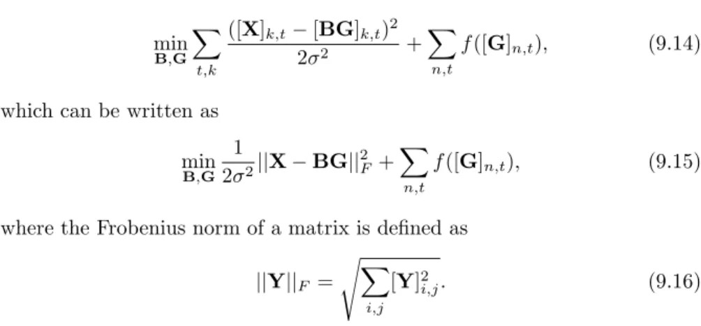
min B,G t,k ([X]k,t−[BG]k,t)2 2σ2 + n,t f([G]n,t), (9.14) which can be written as
min B,G 1 2σ2||X−BG|| 2 F+ n,t f([G]n,t), (9.15) where the Frobenius norm of a matrix is defined as
||Y||F = " i,j [Y]2 i,j. (9.16)
In (9.15), the functionf is used to penalize ‘active’ (non-zero) entries of
G. For example, Olshausen and Field [486] suggested the functions f(x) = log(1 +x2),f(x) =|x|, and f(x) =x2. In audio source separation, Benaroya
et al. [32] and Virtanen [650] have used f(x) = |x|. The prior distribution used by Abdallah and Plumbley [2], [4] corresponds to the function
f(x) = |x|, |x| ≥µ,
µ(1−α) +α|x|, |x|< µ, (9.17)
where the parametersµandαcontrol the relative mass of the central peak in the prior, and the termµ(1−α) is used to make the function continuous atx=
±µ. All these functions give a smaller cost and a higher prior probability for gains near zero. The cost functionf(x) =|x|and the corresponding Laplacian prior p(x) = 12exp(−|x|) are illustrated in Fig. 9.3. Systematic large-scale
evaluations of different sparse priors in audio signals have not been carried out. Naturally, the distributions depend on source signals, and also on the data representation. −2 0 2 0 0.2 0.4 [G] n,t p([ G ] n,t ) −2 0 2 0 1 2 3 [G] n,t f ([ G ] n,t )
Fig. 9.3.The cost functionf(x) =|x|(left) and the corresponding Laplacian prior distributionp(x) = 1
2exp(−|x|) (right). Values ofGnear zero are given a smaller
From (9.15) and the above definitions of f, it can be seen that a sparse representation is obtained by minimizing a cost function which is the weighted sum of the reconstruction error term||X−BG||2
F and the term which incurs a penalty on non-zero elements of G. The variance σ2 is used to balance
between these two. This objective 9.15 can be viewed as a penalized likelihood, discussed in the Tools section (see Sections 2.2.9 and 2.3.3).
Typically,f increases monotonically as a function of the absolute value of its argument. The presented objective requires that the scale of either the basis functions or the gains is somehow fixed. Otherwise, the second term in (9.15) could be minimized without affecting the first term by setting B←Bθ and
G ← G/θ, where the scalar θ → ∞. The scale of the basis functions can be fixed for example with an additional constraint ||bn|| = 1, as done by Hoyer [299], or the variance of the gains can be fixed.
The minimization problem (9.15) is usually solved using iterative algo-rithms. If bothBandGare unknown, the cost function may have several local minima, and in practice reaching the global optimum in a limited time cannot be guaranteed. Standard optimization techniques based on steepest descent, covariant gradient, quasi-Newton, and active-set methods can be used. Differ-ent algorithms and objectives are discussed for example by Kreutz-Delgado et al. [373].
If B is fixed, more efficient optimization algorithms can be used. This can be the case for example when B is learned in advance from training material where sounds are presented in isolation. These methods are discussed in Section 9.6.
No methods have been proposed for estimating the number of sparse com-ponents in a monaural audio signal. Therefore,N has to be set either manu-ally, using some prior information, or to a value which is clearly larger than the expected number of sources. It is also possible to try different numbers of components and to determine a suitable value ofN from the outcome of the trials.
As discussed in the previous section, non-negativity restrictions can be used for frequency-domain basis functions. With a sparse prior and non-negativity restrictions, one has to use the projected steepest descent algo-rithms which are discussed, e.g., by Bertsekas in [35, pp. 203–224]. Hoyer [299], [300] proposed a non-negative sparse coding algorithm by combining NMF and sparse coding. His algorithm used a multiplicative rule to update
B, and projected steepest descent to update G. Projected steepest descent alone is computationally inefficient compared to multiplicative update rules, for example.
In musical signal analysis, sparse coding has been used for example by Abdallah and Plumbley [4], [5] to produce an approximate piano-roll transcription of synthesized harpsichord music and by Virtanen [650] to tran-scribe drums in polyphonic music signals synthesized from MIDI. Also, Blu-mensath and Davies used a sparse prior for the gains, even though their system was based on a different signal model [43]. The framework also enables the use
of further assumptions. Virtanen used a cost function which included a term that favoured the temporal continuity of gains by making large gain changes between adjacent frames unlikely [650].
9.5 Non-Negative Matrix Factorization
As discussed in Section 9.3.2 (see p. 277), it is reasonable to restrict frequency-domain basis functions and their gains to non-negative values. In the signal model X ≈ BG, the element-wise non-negativity of B and G alone is a sufficient condition for the separation of sources in many cases, without an explicit assumption of the independence of the sources.
Paatero and Tatter proposed an NMF algorithm in which the weighted energy of the residual matrixX−BGwas minimized by using a least-squares algorithm where B and G were alternatingly updated under non-negativity restrictions [492]. More recently, Lee and Seung [399, 400] proposed NMF algorithms which have been used in several machine learning tasks since the algorithms are easy to implement and modify.
Lee and Seung proposed two cost functions and estimation algorithms to obtain X ≈ BG [400]. The cost functions are the square of the Euclidean distance deuc and divergence ddiv, which are defined as
deuc(B,G) =||X−BG||2F (9.18) and ddiv(B,G) = k,t D([X]k,t,[BG]k,t), (9.19) where the function D is defined as
D(p, q) =plogp
q −p+q. (9.20)
Both cost functions are lower-bounded by zero, which is obtained only whenX=BG. It can be seen that the Euclidean distance is equal to the first term in (9.15). Minimization of the Euclidean distance leads to a maximum likelihood estimator forBandGin the presence of Gaussian noise. Similarly, minimization of the divergence (9.19) leads to a maximum likelihood estima-tor, when the observations are generated by a Poisson process with mean value [BG]k,t [399]. When
k,t[X]k,t =
k,t[BG]k,t = 1, the divergence (9.19) is equal to the Kullback–Leibler divergence, which is widely used as a distance measure between probability distributions [400].
The estimation algorithms of Lee and Seung minimize the chosen cost function by initializing the entries of B andGwith random positive values, and then by updating them iteratively using multiplicative rules. Each update decreases the value of the cost function until the algorithm converges, i.e., reaches a local minimum. Usually,BandGare updated alternately.
The update rules for the Euclidean distance are given as
B←B.×(XGT)./(BGGT) (9.21) and
G←G.×(BTX)./(BTBG), (9.22) where .×and ./denote the element-wise multiplication and division, respec-tively. The update rules for the divergence are given as
B←B.×(X./BG)G
T
1GT (9.23)
and
G←G.×BT(XB./T1BG), (9.24) where1is an all-onesK-by-Tmatrix, and X
Y denotes the element-wise division of matricesXandY.
To summarize, the algorithm for NMF is as follows:
Algorithm 9.1: Non-Negative Matrix Factorization 1. Initialize each entry ofBandGwith the absolute values of Gaussian noise. 2. UpdateGusing either(9.22)or(9.24)depending on the chosen cost function. 3. UpdateBusing either(9.21)or(9.23)depending on the chosen cost function. 4. Repeat Steps (2)–(3) until the values converge.
Methods for the estimation of the number of components have not been proposed, but all the methods suggested in Section 9.4 are applicable in NMF, too. The multiplicative update rules have proven to be more efficient than for example the projected steepest-descent algorithms [400], [299], [5].
NMF can be used only for a non-negative observation matrix and therefore it is not suitable for the separation of time-domain signals. However, when used with the magnitude or power spectrogram, the basic NMF can be used to separate components without prior information other than the element-wise non-negativity. In particular, factorization of the magnitude spectrogram using the divergence often produces relatively good results. The divergence cost of an individual observation [X]k,tis linear as a function of the scale of the input, since D(αp, αq) =αD(p, q) for any positive scalarα, whereas for the Euclidean cost the dependence is quadratic. Therefore, the divergence is more sensitive to small-energy observations.
NMF does not explicitly aim at components which are statistically in-dependent from each other. However, it has been proved that under certain conditions, the non-negativity restrictions are theoretically sufficient for sep-arating statistically independent sources [525]. It has not been investigated whether musical signals fulfill these conditions, and whether NMF implement
a suitable estimation algorithm. Currently, there is no comprehensive theo-retical explanation of why NMF works so well in sound source separation. If a mixture spectrogram is a sum of sources which have a static spectrum with a time-varying gain, and each of them is active in at least one frame and frequency line in which the other components are inactive, the objec-tive function of NMF is minimized by a decomposition in which the sources are separated perfectly. However, real-world music signals rarely fulfill these conditions. When two or more more sources are present simultaneously at all times, the algorithm is likely to represent them with a single component.
In the analysis of music signals, the basic NMF has been used by Smaragdis and Brown [600], and extended versions of the algorithm have been pro-posed for example by Virtanen [650] and Smaragdis [599]. The problem of the large dynamic range of musical signals has been addressed e.g. by Abdal-lah and Plumbley [5]. By assuming multiplicative gamma-distributed noise in the power spectral domain, they derived the cost function
D(p, q) = p
q −1 + log q
p, (9.25)
to be used instead of (9.20). Compared to the Euclidean distance (9.18) and divergence (9.20), this distance measure is more sensitive to low-energy ob-servations. In our simulations, however, it did not produce results as good as the Euclidean distance or the divergence did.
9.6 Prior Information about Sources
Manual transcription of music requires a lot of prior knowledge and training. The described separation algorithms used some general assumptions about the sources in the core algorithms, such as independence or non-negativity, but also other prior information on the sources is often available. For example in the analysis of pitched musical instruments, it is known in advance that the spectra of instruments are approximately harmonic. Unfortunately, it is difficult to implement harmonicity restrictions in the models discussed earlier. Prior knowledge can also be source-specific. The most common approach to incorporate prior information about sources in the analysis is to train source-specific basis functions in advance. Several approaches have been proposed. The estimation is usually done in two stages, which are
1. Learn source-specific basis functions from training material, such as mono-timbral and monophonic music. Also the characteristics of time-varying gains can be stored, for example by modelling their distribution.
2. Represent a polyphonic signal as a weighted sum of the basis functions of all the instruments. Estimate the gains and keep the basis functions fixed. It is not yet known whether automatic music transcription is possible without any source-specific prior knowledge, but obviously this has the potential to make the task much easier.
Several methods have been proposed for training the basis functions in advance. The most straightforward choice is to also separate the training signal using some of the described methods. For example, Jang and Lee [314] used ISA to train basis functions for two sources separately. Benaroya et al. [32] suggested the use of non-negative sparse coding, but they also tested using the spectra of random frames of the training signal as the basis functions or grouping similar frames to obtain the basis functions. They reported that non-negative sparse coding and the grouping algorithm produced the best results [32]. Gautama and Van Halle compared three different self-organizing methods in the training of basis functions [204].
The training can be done in a more supervised manner by using a sepa-rate set of training samples for each basis function. For example in the drum transcription systems proposed by FitzGerald et al. [188] and Paulus and Virtanen [505], the basis function for each drum instrument was calculated from isolated samples of each drum. It is also possible to generate the basis functions manually, for example so that each of them corresponds to a single pitch. Lepain used frequency-domain harmonic combs as the basis functions, and parameterized the rough shape of the spectrum using a slope parameter [403]. Sha and Saul trained the basis function for each discrete fundamental frequency using a speech database with annotated pitch [579].
In practice, it is difficult to train basis functions for all the possible sources beforehand. An alternative is to use trained or generated basis functions which are then adapted to the observed data. For example, Abdallah and Plumbley initialized their non-negative sparse coding algorithm with basis functions that consisted of harmonic spectra with a quarter-tone pitch spacing [5]. After the initialization, the algorithm was allowed to adapt these.
Once the basis functions have been trained, the observed input signal is represented using them. Sparse coding and non-negative matrix factorization techniques are feasible also in this task. Usually the reconstruction error be-tween the input signal and the model is minimized while using a small number of active basis functions (sparseness constraint). For example, Benaroya et al. proposed an algorithm which minimizes the energy of the reconstruction error while restricting the gains to be non-negative and sparse [32].
If the sparseness criterion is not used, a matrix G reaching the global minimum of the reconstruction error can be usually found rather easily. If the gains are allowed to have negative values and the estimation criterion is the energy of the residual, the standard least-squares solution
ˆ
G= (BTB)−1BTX (9.26)
produces the optimal gains (assuming that the previously trained basis func-tions are linearly independent) [339, pp. 220–226]. If the gains are restricted to negative values, the least-squares solution is obtained using the non-negative least-squares algorithm [397, p. 161]. When the basis functions, observations, and gains are restricted to non-negative values, the global min-imum of the divergence (9.19) between the observations and the model can
be computed by applying the multiplicative update (9.24) iteratively [563], [505]. Lepain minimized the sum of the absolute value of the error between the observations and the model by using linear programming and the Simplex algorithm [403].
The estimation of the gains can also be done in a framework which in-creases the probability of basis functions being non-zero in consecutive frames. For example, Vincent and Rodet used hidden Markov models (HMMs) to model the durations of the notes [648].
It is also possible to train prior distributions for the gains. Jang and Lee used standard ICA techniques to train time-domain basis functions for each source separately, and modelled the probability distribution function of the component gains with a generalized Gaussian distribution which is a family of density functions of the form p(x) ∝ exp(−|x|q) [314]. For an observed
mixture signal, the gains were estimated by maximizing their posterior prob-ability.
9.7 Further Processing of the Components
The main motivation for separating an input signal into components is that each component usually represents a musically meaningful entity, such as a percussive instrument or all the equal-pitched notes of an instrument. Separa-tion alone does not solve the transcripSepara-tion problem, but has the potential to make it much easier. For example, estimation of the fundamental frequency of an isolated sound is easier than multiple fundamental frequency estimation in a mixture signal.
9.7.1 Associating Components with Sources
If the basis functions are estimated from a mixture signal, we do not know which component is produced by which source. Since each source is modelled as a sum of one or more components, we need to associate the components to sources. There are roughly two ways to do this. In the unsupervised classi-fication framework, component clusters are formed based on some similarity measure, and these are interpreted as sources. Alternately, if prior informa-tion about the sources is available, the components can be classified to sources based on their distance to source models. Naturally, if pre-trained basis func-tions are used for each source, the source of each basis function is known and classification is not needed.
Pairwise dependence between the components can be used as a similarity measure for clustering. Even in the case of ICA, which aims at maximizing the independence of the components, some dependencies may remain because it is possible that the input signal contains fewer independent components than are to be separated.
Casey and Westner used the symmetric Kullback–Leibler divergence be-tween the probability distribution functions of basis functions as a distance measure, resulting in an independent component cross-entropy matrix (an ‘ix-egram’) [73]. Dubnov proposed a distance measure derived from the higher-order statistics of the basis functions or the gains [157]. Casey and Westner [73] and Dubnov [157] also suggested clustering algorithms for grouping the components into sources. These try to minimize the inter-cluster dependence and maximize the intra-cluster dependence.
For predefined sound sources, the association can be done using pattern recognition methods. Uhle et al. extracted acoustic features from each com-ponent to classify them either to a drum track or to a harmonic track [634]. The features in their system included, for example, the percussiveness of the time-varying gain, and the noise-likeness and dissonance of the spectrum. An-other system for separating drums from polyphonic music was proposed by Hel´en and Virtanen. They trained a support vector machine (SVM) using the components extracted from a set of drum tracks and polyphonic music sig-nals without drums. Different acoustic features were evaluated, including the above-mentioned ones, mel-frequency cepstral coefficients, and others [282].
9.7.2 Extraction of Musical Information
The separated components are usually analysed to obtain musically important information, such as the onset and offset times and fundamental frequency of each component (assuming that they represent individual notes of a pitched instrument). Naturally, the analysis can be done by synthesizing the com-ponents and by using analysis techniques discussed elsewhere in this book. However, the synthesis stage is usually not needed, but analysis using the ba-sis functions and gains directly is likely to be more reliable, since the syntheba-sis stage may cause some artifacts.
The onset and offset times of each componentn are measured from the time-varying gains gn,t, t = 1. . . T. Ideally, a component is active when its gain is non-zero. In practice, however, the gain may contain interference from other sources and the activity detection has to be done with a more robust method.
Paulus and Virtanen [505] proposed an onset detection procedure that was derived from the psychoacoustically motivated method of Klapuri [347]. The gains of a component were compressed, differentiated, and lowpass filtered. In the resulting ‘accent curve’, all local maxima above a fixed threshold were considered as sound onsets. For percussive sources or other instruments with a strong attack transient, the detection can be done simply by locating local maxima in the gain functions, as done by FitzGerald et al. [188].
The detection of sound offsets is a more difficult problem, since the am-plitude envelope of a note can be exponentially decaying. Methods to be used in the presented framework have not been proposed.
There are several different possibilities for the estimation of the funda-mental frequency of a pitched component. For example, prominent peaks can be located from the spectrum and the two-way mismatch procedure of Maher and Beauchamp [428] can be used, or the fundamental period can be esti-mated from the autocorrelation function which is obtained by inverse Fourier transforming the power spectrum. In our experiments, the enhanced auto-correlation function proposed by Tolonen and Karjalainen [627] was found to produce good results (see p. 253 in this volume). In practice, a component may represent more than one pitch. This happens especially when the pitches are always present simultaneously, as is the case in a chord, for example. No meth-ods have been proposed to detect this situation. Whether or not a component is pitched can be estimated, e.g., from features based on the component [634], [282].
Some systems use fixed basis functions which correspond to certain funda-mental frequency values [403], [579]. In this case, the fundafunda-mental frequency of each basis function is of course known.
9.7.3 Synthesis
Synthesis of the separated components is needed at least when one wants to listen to them, which is a convenient way to roughly evaluate the quality of the separation. Synthesis from time-domain basis functions is straightforward: the signal of componentnin frametis generated by multiplying the basis function
bn by the corresponding gaingn,t, and adjacent frames are combined using the overlap-add method where frames are multiplied by a suitable window function, delayed, and summed.
Synthesis from frequency-domain basis functions is not as trivial. The syn-thesis procedure includes calculation of the magnitude spectrum of a compo-nent in each frame, estimation of the phases to obtain the complex spectrum, and an inverse discrete Fourier transform (IDFT) to obtain the time-domain signal. Adjacent frames are then combined using overlap-add. When magni-tude spectra are used as the basis functions, framewise spectra are obtained as the product of the basis function with its gain. If power spectra are used, a square root has to be taken, and if the frequency resolution is not linear, additional processing has to be done to enable synthesis using the IDFT.
A few alternative methods have been proposed for the phase generation. Using the phases of the original mixture spectrogram produces good syn-thesis quality when the components do not overlap significantly in time and frequency [651]. However, applying the original phases and the IDFT may pro-duce signals which have unrealistic large values at frame boundaries, resulting in perceptually unpleasant discontinuities when the frames are combined us-ing overlap-add. The phase generation method proposed by Griffin and Lim [259] has also been used in synthesis (see for example Casey [70]). The method finds phases so that the error between the separated magnitude spectrogram and the magnitude spectrogram of the resynthesized time-domain signal is
minimized in the least-squares sense. The method can produce good synthesis quality especially for slowly varying sources with deterministic phase behav-iour. The least-squares criterion, however, gives less importance to low-energy partials and often leads to a degraded high-frequency content. The phase gen-eration problem has been recently addressed by Achan et al., who proposed a phase generation method based on a pre-trained autoregressive model [9].
9.8 Time-Varying Components
As mentioned above, the linear model (9.1) is efficient in the analysis of music signals since many musically meaningful entities can be rather well approxi-mated with a fixed spectrum and a time-varying gain. However, representation of sources with strongly time-varying spectrum requires several components, and each fundamental frequency value produced by a pitched instrument has to be represented with a different component. Instead of using multiple com-ponents per source, more complex models can be constructed which allow either a time-varying spectrum or a time-varying fundamental frequency for each component. These are discussed in the following two subsections.
9.8.1 Time-Varying Spectra
Time-varying spectra of components can be obtained by replacing each basis functionbnby a sequence of basis functionsbn,τ, whereτ = 0. . . L−1 is the frame index. If a frequency-domain representation is used, this means that a static short-time spectrum of a component is replaced by a spectrogram of lengthLframes.
The signal model for one component can be formulated as a convolution between its spectrogram and time-varying gain. The model for a mixture spectrum ofN components is given by
xt≈ N n=1 L−1 τ=0 bn,τgn,t−τ. (9.27)
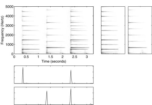
The model can be interpreted so that each componentnconsists of repetitions of an event which has a spectrogrambn,τ,τ= 0...L−1. Each non-zero value of the time-varying gaingn,t denotes an onset of the event and the value of the gain gives the scaling factor of each repetition. A simple two-note example is illustrated in Fig. 9.4.
The parameters of the convolutive model (9.27) can be estimated using methods extended from NMF and sparse coding. In these, the reconstruction error between the model and the observations is minimized, while restricting the parameters to be entry-wise non-negative. Also favouring sparse gains is clearly reasonable, since real-world sound events set on in a small number of
Time (seconds) Frequency (Hertz) 0 0.5 1 1.5 2 2.5 3 0 1000 2000 3000 4000 5000
Fig. 9.4. An example of the convolutive model (9.27) which allows time-varying components. The mixture spectrogram (upper left panel) contains the notes C#6 and F#6 of the acoustic guitar, first played separately and then together. The upper right panels illustrate the learned note spectrograms and the lower panel shows their time-varying gains. In the gains, an impulse corresponds to the onset of a note. The components were estimated using a modified version of the algorithm proposed by Smaragdis in [599]. In the case of more complex signals, it is difficult to obtain such clear impulses.
frames only. Virtanen [651] proposed an algorithm which is based on non-negative sparse coding, whereas that of Smaragdis [599] aims at minimizing the divergence between the observation and the model while constraining non-negativity.
Arbitrarily long durations L may not be used if the basis functions are estimated from a mixture signal. When N L≥T, the input spectrogram can be represented perfectly as a sum of concatenated event spectrograms (without separation). Meaningful sources are likely to be separated only whenN L≪T. In other words, estimation of several components with largeL requires long input signals.
In addition, the method proposed by Blumensath and Davies [43] can be formulated using (9.27). Their objective was to find sparse and shift-invariant decompositions of a signal in the time domain. Their model allows an event to begin at any time with one sample accuracy which makes the number of free parameters in the model large. To reduce the dimensionality of the problem, Blumensath and Davies proposed an algorithm which carried out
the optimization in a subspace of the parameters. They also included a sparse prior for the gains.
9.8.2 Time-Varying Fundamental Frequencies
In some cases, it is desirable to use a model which can represent different pitch values of an instrument with a single component. For example, in the case where a note with a certain pitch is present only during a short time, separating it from co-occurring sources is difficult. However, if other notes of the source with adjacent pitch values can be utilized, the estimation becomes more reliable.
Varying fundamental frequencies are difficult to model using time-domain basis functions or frequency-domain basis functions with linear frequency reso-lution. This is because changing the fundamental frequency of a basis function is a non-linear operation which is difficult to implement in practice: if the fun-damental frequency is multiplied by a factorγ, the frequencies of the harmonic components are also multiplied byγ; this can be viewed as a stretching of the spectrum. For an arbitrary value ofγ, the stretching is difficult to perform on a discrete linear frequency resolution, at least using a simple operator which could be used in the unsupervised learning framework. The same holds as well for time-domain basis functions.
A logarithmic spacing of frequency bins makes it easier to represent varying fundamental frequencies. A logarithmic scale consists of discrete frequencies frefβk−1, wherek= 1. . . K is the discrete frequency index,β >1 is the ratio
between adjacent frequency bins, and fref is a reference frequency in Hertz
which can be selected arbitrarily. For example,β= 12√
2 produces a frequency scale where the spacing between the frequencies is one semitone.
On the logarithmic scale, the spacing of the partials of a harmonic sound is independent of its fundamental frequency. For fundamental frequency f0,
the overtone frequencies of a perfectly harmonic sound aremf0, wherem >0
is an integer. On the logarithmic scale, the corresponding frequency indices are k= logβ(m) + logβ(f0/fref), and thus the fundamental frequency affects
only the offset logβ(f0/fref), not the intervals between the harmonics.
Given the spectrumX(k) of a harmonic sound with fundamental frequency
f0, a fundamental frequency multiplication γf0 can be implemented simply
as a translation ˆX(k) =X(k−δ), whereδ is given byδ= logβγ. Compared with the stretching of the spectrum, this is usually easier to implement.
The estimation of harmonic spectra and their translations can be done adaptively by fitting a model onto the observations.4 However, this is
diffi-cult for an unknown number of sounds and fundamental frequencies, since the reconstruction error as a function of translation δ has several local minima
4
This approach is related to the fundamental frequency estimation method of Brown, who calculated the cross-correlation between an input spectrum and a single harmonic template on the logarithmic frequency scale [54].
at harmonic intervals, which makes the optimization procedure likely to be-come stuck in a local minimum far from the global optimum. A more feasible parameterization allows each component to have several active fundamental frequencies in each frame, the amount of which is to be estimated. This means that each time-varying gaingn,tis replaced by gainsgn,t,z, wherez= 0, . . . , Z is a frequency-shift index andZis the maximum allowed shift. The gaingn,t,z describes the amount of thenth component in frame tat a fundamental
fre-quency which is obtained by translating the fundamental frefre-quency of basis functionbn byz indices.
The size of the shiftzdepends on the frequency resolution. For example, if 48 frequency lines within each octave are used (β = 48√
2),z= 4 corresponds to a shift of one semitone. For simplicity, the model is formulated to allow shifts only to higher frequencies, but it can be formulated to allow both negative and positive shifts, too.
A vectorgn,t=gn,t,0, . . . , gn,t,ZT is used to denote the gains of compo-nentnin framet. The model can be formulated as
xt≈ N
n=1
bn∗gn,t, t= 1. . . T, (9.28)
where∗ denotes a convolution operator, defined between vectors as
b=bn∗gn,t⇔bk= Z
z=0
bn,k−zgn,t,z, k= 1. . . K. (9.29) Figure 9.5 shows the basis function and gains estimated from the example signal in Fig. 9.1. In general, the parameters can be estimated by fitting the model to observations with certain restrictions, such as non-negativity or sparseness. Algorithms for this purpose can be derived by extending those used in NMF and sparse coding. Here we present an extension of NMF, where the parameters are estimated by minimizing the divergence (9.19) between the observationsXand the model (9.28), while restricting the gains and basis functions to be non-negative.
The elements ofgn,t andbn are initialized with random values and then updated iteratively until the values converge. To simplify the notation, let us denote the model with current parameter estimates byvt=
N
n=1bn∗gn,t,
t= 1. . . T. The update rule for the gains is given as
gn,t←gn,t.× bn⋆( xt vt) bn⋆1 , (9.30)
where 1 is a K-length vector of ones and ⋆ denotes the correlation of vec-tors, defined for real-valued vectors bn and y as g = bn ⋆ y ⇔ gz = K
k=1bn,kyk+z, z = 0, . . . , Z. The update rule for the basis functions is given as
bn ←bn.× T t=1(gn,t⋆ xt vt) gn,t⋆1 . (9.31)
The overall optimization algorithm for non-negative matrix deconvolution is as follows:
Algorithm 9.2: Non-Negative Matrix Deconvolution 1. Initialize eachgn,tandbnwith the absolute values of Gaussian noise. 2. Calculatevt= N
n=1bn∗gn,tfor eacht= 1. . . T.
3. Update eachgn,tusing(9.30). 4. Calculatevtas in Step 2.
5. Update eachbnusing(9.31). Repeat Steps (2)–(5) until the values converge.
The algorithm produces good results if the number of sources is small, but for multiple sources and more complex signals, it is difficult to get as good
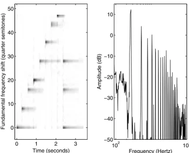
Time (seconds)
Fundamental frequency shift (quarter semitones)
0 1 2 3 0 10 20 30 40 50 102 104 −50 −40 −30 −20 −10 0 10 Frequency (Hertz) Amplitude (dB)
Fig. 9.5.Illustration of the time-varying gains (left) and the basis function (right) of a component that was estimated from the example signal in Fig. 9.1 containing a diatonic scale and a C major chord. On the left, the intensity of the image rep-resents the value of the gain at each fundamental frequency shift and frame index. Here the fundamental frequencies of the notes can be seen more clearly than from the spectrogram of Fig. 9.1. The parameters were estimated using the algorithm proposed in this section.
results as those illustrated in Fig. 9.5. The model allows all the fundamental frequencies within the rangez= 0. . . Zto be active simultaneously, thus, it is not restrictive enough. For example, the algorithm may model a non-harmonic drum spectrum by using a harmonic basis function shifted to multiple adjacent fundamental frequencies. Ideally, this could be solved by restricting the gains to be sparse, but the sparseness criterion complicates the optimization.
In principle, it is possible to combine varying spectra and time-varying fundamental frequencies into the same model, but this further in-creases the number of free parameters so that it can be difficult to obtain good separation results.
When shifting the harmonic structure of the spectrum, the formant struc-ture becomes shifted, too. Therefore, representing time-varying pitch by trans-lating the basis function is appropriate only for nearby pitch values. It is unlikely that the whole fundamental frequency range of an instrument could be modelled by shifting a single basis function.
9.9 Evaluation of the Separation Quality
A necessary condition for the development of source separation methods is the ability to measure the quality of their results. In general, the separation quality can be measured by calculating the error between the separated sig-nals and reference sources, or by listening to the separated sigsig-nals. In the case that separation is used as a pre-processing step for automatic music tran-scription, the quality should be judged according to the final application, i.e., the transcription accuracy.
Performance measures for audio source separation tasks have been dis-cussed, e.g., by Gribonval et al. [258]. They proposed measures estimating the amount of interference from other sources and the distortion caused by the separation algorithm. Many authors have used the signal-to-distortion ratio (SDR) as a simple measure to summarize the quality. This is defined in deci-bels as SDR [dB] = 10 log10 ts(t) 2 t[ˆs(t)−s(t)]2 , (9.32)
wheres(t) is a reference signal of the source before mixing, and ˆs(t) is the sep-arated signal. In the separation of music signals, Jang and Lee [314] reported average SDR of 9.6 dB for an ISA-based algorithm which trains basis func-tions separately for each source. Hel´en and Virtanen [282] reported average SDR of 6.4 dB for NMF in the separation of drums and polyphonic harmonic track, and a clearly lower performance (SDR below 0 dB) for ISA.
In practice, quantitative evaluation of the separation quality requires that reference signals, i.e., the original signals s(t) before mixing, be available. In the case of real-world music signals, it is difficult to obtain the tracks of each individual source instrument and, therefore, synthesized material is often used.
Generating test signals for this purpose is not a trivial task. For example, ma-terial generated using a software synthesizer may produce misleading results for algorithms which learn structures from the data, since many synthesiz-ers produces notes which are identical at each repetition. In the case that source separation is a part of a music transcription system, quality evaluation requires that audio signals with an accurate reference notation are available (see Chapter 11, p. 355). Large-scale comparisons of different separation al-gorithms for music transcription have not been made.
9.10 Summary and Discussion
The algorithms presented in this chapter show that rather simple principles can be used to learn and separate sources from music signals in an unsuper-vised manner. Individual musical sounds can usually be modelled quite well using a fixed spectrum with time-varying gain, which enables the use of ICA, sparse coding, and NMF algorithms for their separation. Actually, all the al-gorithms based on the linear model (9.4) can be viewed as performing matrix factorization; the factorization criteria are just different.
The simplicity of the additive model makes it relatively easy to extend and modify it, along with the presented algorithms. However, a challenge with the presented methods is that it is difficult to incorporate some types of restrictions for the sources. For example, it is difficult to restrict the sources to be harmonic if they are learned from the mixture signal.
Compared to other approaches towards monaural sound source separa-tion, the unsupervised methods discussed in this chapter enable a relatively good separation quality—although it should be noted that the performance in general is still very limited. A strength of the presented methods is their scalability: the methods can be used for arbitrarily complex material. In the case of simple monophonic signals, they can be used to separate individual notes, and in complex polyphonic material, the algorithms can extract larger repeating entities, such as chords. Some of the algorithms, for example NMF using the magnitude spectrogram representation, are quite easy to imple-ment. The computational complexity of the presented methods may restrict their applicability if the number of components is large or the target signal is long.
Large-scale evaluations of the described algorithms on real-world poly-phonic music recordings have not been presented. Most published results use a small set of test material and the results are not comparable with each other. Although conclusive evaluation data are not available, a preliminary experience from our simulations has been that NMF (or sparse coding with non-negativity restrictions) often produces better results than ISA. It was also noticed that prior information about sources can improve the separation quality significantly. Incorporating higher-level models into the optimization
algorithms is a big challenge, but will presumably lead to better results. Con-trary to the general view held by most researchers less than 10 years ago, unsupervised learning has proven to be applicable for the analysis of real-world music signals, and the area is still developing rapidly.