e-Publications@Marquette
Management Faculty Research and Publications Management, Department of
1-1-2013
Rule Based Forecasting [RBF] - Improving Efficacy
of Judgmental Forecasts Using Simplified Expert
Rules
Monica Adya
Marquette University, [email protected]
Edward J. Lusk SUNY Plattsburgh
Published version.International Research Journal of Applied Finance, Vol. IV, No. 8 (August 2013): 1006-1024.Publisher Link. © 2013 Kaizen Publications. Used with permission.
1006
Rule Based Forecasting [RBF] - Improving Efficacy of Judgmental Forecasts
Using Simplified Expert Rules
+Monica Adya, PhD
Department of Management, Marquette University, Milwaukee WI, USA [email protected]
Edward J. Lusk*, PhD, CPA Professor of Accounting
The State University of New York (SUNY) at Plattsburgh School of Business and Economics: Plattsburgh, NY, USA
[email protected] Term Visiting Scholar 2013-2014
Leuphana Universität Lüneburg, Germany
and
Emeritus, Department of Statistics
The Wharton School, University of Pennsylvania, Philadelphia, PA, USA
+We wish to thank Professor Fred Collopy, Weatherhead School of Management; Case Western Reserve University, Cleveland Ohio, USA for his assistance during the developmental phase of this study and Herr Manuel Bern, Professional, Forensic & Dispute Services; Germany Deloitte & Touche, GmbH, Frankfurt, Germany for his careful reading and helpful comments.
1007
Abstract
Rule-based Forecasting (RBF) has emerged to be an effective forecasting model compared to well-accepted benchmarks. However, the original RBF model, introduced in1992, incorporates 99 production rules and is, therefore, difficult to apply judgmentally. In this research study, we present a core rule-set from RBF that can be used to inform both judgmental forecasting practice and pedagogy. The simplified rule-set, called coreRBF, is validated by asking forecasters to judgmentally apply the rules to time series forecasting tasks. Results demonstrate that forecasting accuracy from judgmental use of coreRBF is not statistically different from that reported from similar applications of RBF. Further, we benchmarked these coreRBF forecasts against forecasts from (a) untrained forecasters, (b) an expert system based on RBF, and (c) the original 1992 RBF study. Forecast accuracies were in the hypothesized direction, arguing for the generalizability and validity of the coreRBF rules.
Keywords: Time Series, RBF, Rule Reduction, Comparative Analysis, Expert System Efficacy
I. Introduction and Motivations
In most areas of finance, production, and logistics, well-designed and validated rule-based systems can significantly impact the quality of decision making process. Such rule-based systems: (1) represent the “codification of knowledge and decision rules of experts” (Shanteau and Stewart, 1992, p. 101), (2) link related information to automate deductive capabilities (Ramsey, et al. 1986; Angeli, 2010), and (3) encode heuristics in a simple and uniform manner (Clancey, 1983; Angeli, 2010). Much of this is done to provide problem-solving support for simpler, procedural functions in specific domains while freeing up experts to undertake more advanced and unstructured problems (Clancey, 1983). From another perspective, in particular noting the early works of Herb Simon (Simon, 1980), rule-based systems are said to effectively model and improve human reasoning and provide teaching mechanisms to improve judgmental decision making (Clancey, 1983; Adya, Lusk, and Belhadjali, 2009). Both aspects clearly offer benefits in most domains where accurate projections of the future offer tactical and strategic advantages, as exemplified by important linkages between forecasting and firm efficacy and competitive advantage (Mohammad, Anvari and Saberi, 2013; Kalinga, Lonseth, and Lonseth, 2013). Accepting as evident that forecasting is pivotal for sound organizational planning, the second aspect, which is improvement in judgmental decision making related to forecasting, is the key driver for this study.
In the forecasting literature, Rule-based Forecasting (RBF), developed and extensivelyvalidated by Collopy and Armstrong (1992), hereafter referred to as C&A, is indisputably the most replicated and extended expert system designed to support time series forecasting tasks (see Adya, et al. 2000; Adya, et al. 2001; Adya, et al, 2009). The original RBF uses 99 “IF…THEN…” coding rules to integrate judgment with procedures that weight and combine forecasts from four statistical forecasting methods to generate rule-based forecasts. Eighteen features of time series are used to assign these weights to generate customized RBF forecasts for each series. These rules were developed and validated based on four decades of empirical knowledge, surveys of forecasting practitioners and academics, and protocol analysis of five leading academics and domain experts. C&A (1992) validated and tested RBF on 126 annual economic and demographic time series where it outperformed other well-accepted benchmarks. Subsequent application of RBF on additional data sets (see Adya, et al. 2000, 2001) has further established its validity as an effective forecasting model (Makridakis and Hibon, 2000).
1008 However, RBF has a large set of 99 rules, making it challenging to use the embedded expert knowledge as a training tool to improve judgmental forecasting practice and pedagogy. As C&A note in their concluding comments:
“The rule-based forecasting procedure offers promise. We provide our rules as a starting point. Hopefully, they will be replaced by simpler and fewer rules”. p.1408
This vision underlies the motivations for this study.
Motivations for Rule Simplification and Reduction
Forecasters often use judgment to either produce forecasts or adjust forecasts produced by statistical methods (Sanders and Ritzman, 1992). Often, these judgmental processes are biased or limited by human information processing capabilities, causing forecasters to see patterns where none exist (O’Connor, Remus, and Griggs, 1993) and, thereby, compromise accuracy. A simple set of rules, essentially operational guidelines, could potentially mitigate this dysfunction by focusing judgmental processes on the most relevant forecasting knowledge. With its extensive knowledge base, RBF can potentially yield such gains. Yet, ironically, despite its superior performance in forecasting practice, the RBF model has not had a major impact on forecasting pedagogy and judgmental decision making, essentially due to the demands imposed by 99-rules and the related feature-set needed to parameterize these rules. A reduced rule-set can address this limitation and uncover opportunities for improving forecasting practice.
Thus the purpose of this study is to identify a smaller, pragmatic, yet effective set of RBF-rules that could be readily comprehended by a group of non-expert, but likely, users as they employ models that require judgmental interventions. The essential issue to be determined, however, is whether the loss in forecast accuracy from reduction of RBF rules could be offset by improved judgmental application of the simplified rule-set. Key benefits expected for this rule-reduction, then, are:
1. Reduced rules could be used by forecasters to deliver improved unaided judgments in shorter time, thereby increasing efficiency in domains where logistical imperatives demand timely yet effective actions, as is the case for dynamic financial markets (e.g. Chang, Jimenez-Martin, McAleer, and Amaral, 2013)
2. Improvements may also been seen through reductions in the number of time series features that forecasters need to evaluate in order to produce forecasts, thereby further increasing efficiency at the point of forecast.
3. Fewer rules and features could improve forecasting adjustment behaviors and reduce dysfunctional adjustments by minimizing confusion stemming from contradictory interactions between time series cues.
4. A smaller core set of forecasting rules could be easily embedded within a forecasting support system (FSS) to improve system-driven outcomes with positive implications for improved allocation of human resources.
5. Finally, these simplifications may propagate the use of structured forecasting knowledge by initially making it accessible and usable for corporate training as well as for academic domains heavily dependent on forecasting such as finance (Korol, 2013), production (Tiacci and Saetta, 2012; Kim, Hong and Koo, 2013) and logistics and supply-chain (Shukla and Jharkharia, 2013).
In the next section, we provide a background to forecasting systems, specifically RBF. We then describe the process by which we arrived at the core set of rules followed by the design and execution of our validation studies. The paper concludes with discussion of results, recommendations for practice, and implications for future research in this aspect of forecasting.
1009
II Background
The nature and character of forecasting have changed dramatically over the past several decades. In the 1960s, the computer and its empowering processing capabilities offered easy access to even the most complicated mathematically- and statistically-driven forecasting models and systems. This resulted in an unprecedented proliferation of forecasting models that demanded a comparative evaluation of situational effectiveness i.e., identifying conditions under which a particular forecasting method may produce more accurate forecasts than others. This environment spawned a series of forecasting competitions, the most comprehensive of which was the Makridakis Competition (Makridakis, et al. 1982), referred to as the M-Competition. The M-Competition tested the performance of a range of forecasting methods on a common and extensive set of data and, in the process, produced surprising results which called into question the efficacy of a wide range of modeling systems, including for instance, even the well-established ARIMA/Box-Jenkins models. It also drew attention to: (1) the benefit of simple models and (2) of combining forecasts from multiple methods (Clemens, 1989), resulting in major developments that shifted emphasis to combining forecasts from multiple methods and, more significantly, combining judgment with statistics, one significant outcome of which was RBF.
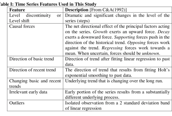
The original RBF, as developed by C&A, used 99 “IF…THEN…” rules to integrate judgmental and statistical procedures that combine forecasts from four simple and well-accepted forecasting models: Random Walk, OLS-Linear Regression, Holt’s Exponential Smoothing, and Brown’s Exponential Smoothing. These four models were central to the 99RBF rules and forecasts from these models were subsequently combined based upon weight parameters determined from a complex interaction of time series features such as direction of basic and recent trends, variation around the trend, level discontinuities, and suspicious patterns (see Table I). For illustration, two rules from RBF are presented below (items in bold are features of time series).
IF the direction of the basic trend AND the direction of the recent trend are not the same OR if the trends agree with one another but differ from the causal forces, THEN add 15% to the weight on the Random Walk and subtract it from that on the other trend estimates.
IF there is an unstable recent trend, THEN add 20% to the weight on the Random Walk and subtract it from that on Brown's and Holt's.
Refer Table I
In the 99 rules, RBF captured over four decades of significant forecasting knowledge. In addition to being central to this expert system, its rule-based knowledge held promise for informing, and thereby improving, judgmental forecasts. In fact, Adya, et al. (2009) provide evidence for its effectiveness in informing judgmental practice for non-expert, but dedicated and instructed, user groups. However, this study also found pragmatic limitations in pedagogical use of this extensive knowledge-base. Considering limitations of human information processing (Cowan, 1988; Adya and Lusk, 2012), the size of this rule set was a significant deterrent for its utilization towards improved judgmental forecasting.
Following the challenge offered by C&A to simplify RBF, the first rule-set refinement was carried out by Adya (2000) who, in collaboration with C&A, corrected some of the initial RBF rules and, thereafter, presented a simplified version of RBF with elimination of rules related to Brown’s exponential smoothing (Adya, et al. 2001). The Brown reduced model performed well
1010 using only 65 percent of the initial 99 rules. This altered version of the RBF model will be referred to as ARBF. As part of that study, the ARBF rules and several time series feature detection modules were automated and coded into an expert system, hereon referred to as to the ARBF-Expert System (ARBF-ES). Forecasts from this system are also used as one of benchmarks in this study. While ARBF-ES was less accurate than the original RBF,as expected, the automation significantly reduced temporal demands and variability by reducing input from human processes. Adya et al. (2001) note:
“Accuracy for 30% of the 122 annual time series was similar to that reported for RBF. For the remaining series, there were as many that did better with automatic feature detection as there were those do worse. In other words, the use of automated feature detection heuristics reduced costs of using RBF without negatively affecting forecast accuracy.” Abstract citation.
ARBF still contained over 60 rules and therefore continued to pose challenges for application to judgmental forecasting. Furthering C&As call for investigation into possible reductions, this study was designed to move closer to a more basic, yet essential, set of RBF rules. The process of arriving at a proposed core set of rules, i.e. a Reduced RBF model, and testing of its effectiveness and efficiency in a forecasting setting is described next.
III Reducing and Validating the RBF to coreRBF
For identifying this core rule set, we began with ARBF as it stood after incorporating the corrections reported in Adya (2000) and reduction of rules related to Brown’s exponential smoothing presented in Adya et al. (2001). Both authors of this current study independently selected the rules that each believed to be the core set of rules. In doing so, we relied on sensitivity analyses and findings from prior RBF studies. For instance, Armstrong and Collopy (1993) found that the use of a rule related to causal forces improved forecasts for 20 series. Similarly, C&A found that RBF produced more accurate forecast than benchmarks under conditions of instability (e.g. presence of level discontinuities, changes in basic trend, etc) and uncertainty (e.g. variation around the trend). These findings were confirmed in later studies in Adya, et al. (2000) and Adya, et al. (2001). By relying on these prior empirical studies, each author arrived at 15 rules, some of which were identical, others that related to the same set of underlying features (e.g. rules related to level discontinuities), and a few rules that were relatively different (e.g., rules related to suspicious patterns in time series). Through discussion, the authors reconciled most of these differences. In cases where a strong argument could not be positioned in favor or against a rule, the final decision was made by the first author because of her extensive engagement with the RBF system and its underlying feature characteristics. The reconciled rules were evaluated by one of the original C&A authors, based upon which we adjusted the reduced rule set and converged to 12 rules, presented in the Appendix and hereon referred to as coreRBF.
The 12 coreRBF rules, as a sub-set of the original 99 rules, are related to calibration of the short and long models. Short model generates forecasts for the first period out i.e., one-ahead forecasts while the long-model generates forecasts for the last forecast period, n. Following C&A, for annual series, n is set at 6 years. Forecasts between the 1st and 6th period are generated by blending the short and long model forecasts, rules for which are presented in C&A. The 12 rules in the appendix provide the only calibration that was used to modify the initial weights for the four decomposed parts: the Short Model Level, the Short Model Trend, the Long Model Level, and the Long Model Trend just as were used in the original 99 C&A rules.
1011 The three models used to generate the forecasts to be combined are:
1. Random Walk [RW]: This is the last data point in the historical series that is projected out as forecasts for all forecast periods, 1st to nth. As such, random walk forecasts assume that whatever occurred in the last historical period will continue to occur during the time periods to be forecasted. The Level is the RW value and so the Trend is by definition zero (0). The Random Walk is also referred to as The Naïve method.
2. Linear Regression [LR]: This is the OLS two-parameter linear model. The Level is the regression value at the historicallast data point; the Trend is the Slope of the regression equation as fitted.
3. Holt’s Exponential Smoothing [HES]: This is a linear two parameter exponential smoothing model and is also the ARIMA (0,2,2). Computationally, for the ARBF and the coreRBF models, the Fitted Holt model is used to form the Level as the Holt value at the last data point in the historical series to be forecasted, and the Trend is the average of the Holt values over the projection period.
Table II combines these elements, weights and forecasting models, to present the starting weights used by C&A (see also the Appendix). Forecasters would begin with three sets of forecasts for time series level and trend – one set from each of the three methods described above. Initially, these forecasts would be combined using these initialweights listed below 40% of the forecast value would come from RW, 20% from OLS-Regression, and 40% from HES. These weights would then be adjusted based on the application of the 12 rules offered in the Appendix.
Refer Table II
Adjustments to these initial weights are made as for the original C&A rule-set. For instance, for Rule 40 from the appendix, presented below,
Rule 40: Causal Forces Unknown (Short Model Trend)
IF the causal forces are unknown, THEN add 0.05 to the weight on the Random Walk and subtract it from that on the Linear Regression trend estimate.
0.05 is added to the initial weight of the Random Walk and simultaneously subtracted from Linear Regression resulting in a weight of 0.45 [0.40 + 0.05] for Random Walk and 0.35 [0.40 −
0.05] for Linear Regression. This, of course, is logical because if the underlying Causal Forces, i.e. net effect of factors shaping the future direction of a series, are not known, forecasters are bound to have lower confidence in the OLS regression basictrend in favor of a random effect. In summary, as there are fewer rules, fewer feature computations, and as such, fewer considerations in developing coreRBF forecasts, judgmental application of these rules is expected to be more efficient and less time consuming but, of course,not as accurate as when making use of the full ARBF rule-set. This trade-off is tested and reported in the next sections.
III General Data Preparation Steps
There are certain data preparation steps that apply equallyto the coreRBF, ARBF, and the C&A rule-based models. For instance, the features: irrelevant early data, outliers, and functional form of the time series are adjusted or accommodated for prior to application of the forecasting method. The following data modification steps suggested by C&A are also followed in this study:
1012 1.) Irrelevant Early Data: Typically, this occurs in the “start-up” of a generating process, for example, in the first few years of an organization before the channels of distribution or market presence becomes well-established. Irrelevant early data, as per C&A, can be eliminated by a direct reduction of such data from the time series, thereby resulting in a shorter series.
2.) Outliers: If a data point in a time series is identified as a residual point outside the 95% confidence interval (CI) of the OLS Regression, the point is flagged as an outlier and is replaced with the directional point of the 95% CI.
3.) Functional Form: Functional form of the underlying generating process can be additive or multiplicative. Additive is selected if the variance of the time series is apparently independent from its level and is unchanging over time. That is to say the variance band is a constant function over time for the realized time series for any set of random discreet windows relative to the level. If this is not the case, the series is assumed to be multiplicative, suggesting the ln() transformation and exp() re-transformation be used, where is the time series vector. In the case where there is doubt, the multiplicative transformation is preferred as it is more neutral than the additive functional form.
Forecast accuracy was measured using the well-accepted Absolute Percentage Error (APE) and Relative Absolute Error (RAE) error measures as suggested in Armstrong and Collopy (1992) and as done for all RBF studies referenced in this paper.
Specifically, the APE and the RAE are computed as:
APEh = |Fm,h− Ah| / Ah (1)
RAEh = |Fm,h− Ah| / | RWh−Ah| (2)
where: , represents the Forecast using model m, for time horizon h, represents the Actual or realized observation for time horizon h,
represents the Forecast using the Random Walk model for time horizon.
According to Armstrong and Collopy (1992) these measures provide independent theoretical views of forecast error and minimize biases stemming from a tendency to favor methods that perform well on selected error measures. Consistent with their recommendations, APE and RAE are winsorized between 0.01 and 10.0. Specifically, if APE or RAE < 0.01, then a value of 0.01 was used as the replacement while if APE or RAE > 10.0 then a value of 10 was used as the replacement. All measures reported were medians, i.e. Median APE (MdAPE) and Median RAEs (MdRAE). Finally, all p-values reported in data tables are two-tailed computed using the Median Test, JMP/SAS;v.10.
IV Experimental Design and Hypothesis
The coreRBF rule-set was tested on graduate student participants enrolled in a forecasting course at the Otto-von-Guericke University (OVG) in Germany in 2009. This course has been taught as a RBF course for six years in the International Master Degree program in Economics. The typical mix of students is 30% German, 30% from other EU and Balkan block countries, 25% from China and Japan, and 15% from the USA and South America. The language of instruction is English and the second author, who delivered this course, is a native speaker. The experimental design used a judgmental testing of coreRBF with the OVG students. Specifically, participants were asked to apply the 12 coreRBF rules to generate judgmental forecasts for given time series. Their forecast accuracy was compared with several benchmarks, discussed later in this section.
1013
The Subjects In 2009, 24 participants completed the course using as the text: Hanke, Wichern and Reitsch (2001)42. They were engaged in a two-stage sequential application of forecasting knowledge to the given tasks. Every participant was randomly assigned two forecasting sets, each comprised of three series, from a subset of 12 series from the M-Competition data. They had to produce judgmental forecasts for one set of series using the 12 rules from coreRBF and later for the other, using the 65 ARBF rules from Adya, et al. (2001), i.e. the ARBF model. The order of application of ARBF or the coreRBF was quasi-randomly assigned43 so as to arrive at 50% of the students’ first using coreRBF and then ARBF, and the remaining using ARBF first and then coreRBF. The two sets of time series were different for each participant, thus no participant used the two rule-sets on the same series. As was the practice for all the previous years, prizes were awarded for most accurate overall forecasts, i.e., across all six series from the two sets. First and second place awards were given to each of the two groups that: (a) first used ARBF and then coreRBF and (b) first used coreRBF and then ARBF. The prizes were 50€ and 25€ each for first and second places, 150€ in total. If participants felt that a series was too difficult to forecast for any reason, they had the option of not forecasting the series. Two students made that election and submitted four, rather than six, series. This yielded a total of 840 forecasts: [Students x Series x Forecasts per series]: [(22 x 6 x 6) + (2 x 4 x 6)].
Logistics of the Design The central design decision was to have participants serve as their own control and, thereby, control for individual performance differentials. As such, we used a “balanced” random order application design [ROAD]. Therein, the central control test is against an order effect. A participant was, first, randomly assigned either the coreRBF or the ARBF rules and series to forecast. After the forecasts were completed, the next day, the same individual was assigned the other model and another set of series to forecast. For example, Participant 20 first was assigned series 13, 14, and 15 to forecast using coreRBF44. After completion, the next day she was assigned series 2, 5, and 9 to forecast using ARBF. The forecasting assignment was done over two days of a weekend in a supervised, dedicated computer lab using the JMP software for statistical analyses (Sall, Lehman and Creighton, 2001). Six hours of “task” time were reserved for each of the two days, not including a mandatory midday break for 90 minutes. Each participant had a dedicated computer. No student requested additional time, in spite of being given the option. The instructor was available to answer any questions during the time participants were executing the tasks. Participants mostly asked questions pertaining to (i) definitions of features, (ii) meaning of specific wording of rules, and (iii) functionality of the JMP software.
IV.A Comparative Benchmarks
Judgmental forecasts generated by the OVG participants using the 12 coreRBF rules formed the experimental data and are referred to as coreRBF-Judgment. To assess the representativeness
42
The APEs and RAEs error measures were used to test for grade effects, as is the practice when using students. We partitioned the participants into two groups based upon median assigned final course grades. No APE or RAE differences were found at a p-value < 0.25 between the two grade groups.
43
Quasi in this context meant that we first randomly assigned 75% the RBFcoreRBF or coreRBFRBF sequencing and then selectively used the remaining 25% to ensure that 50% of the participants had one or the other application sequence without receiving the same series that they had for the intake judgments.
44 These series were not noted by the numbers used in C&A. We developed a special neutral coding assigning
1014 and generalizability of the rules underlying these forecasts, coreRBF-Judgment forecasts were evaluated relative to those generated by the same participants using the ARBF rule set from Adya et al. (2001) (referred to as ARBF-Judgment) as well as a set of well-validated benchmarks described below:
Benchmark 1 – Untrained Forecasts: The most basic benchmarks were forecasts from untrained participants who had no exposure to either ARBF or coreRBF rules. For this benchmark, the incoming OVG students were asked to generate forecasts on the day their course began i.e., before any training or instruction was delivered. The students were given three series selected randomly from the same set of series used with the experimental group. They had 45 minutes to produce one- to six-period-ahead forecasts for all the three series. No instructions were provided but they were permitted to use whatever forecasting methods that they deemed useful in making the forecasts. Participants were informed that these initial forecasts were to be used later in the course and, as such, to take care in producing the best forecasts that they could. They were also given the option of generating these forecasts over the weekend. Over the approximately 150 students taught over the years, only one student has taken the work home. Most students used simple heuristics such as projecting a hand-drawn line and locating the forecasting point using the sketched line as a guide. Rarely did students use a formula-driven approach. In a few instances students did simple averaging of past values, simulating the Moving Average model. These initial forecasts are referred to as Untrained Forecasts.
Benchmark 2 – ARBF Expert System Forecasts: Using the ARBF rule-set presented in Adya, et al. (2001), an expert system was developed, calibrated, and validated in Adya, et al. (2000, 2001). This system also contained the automated time-series feature detection routines referred to earlier. This ARBF-ES expert system provided a systems-driven benchmark that is unconstrained by limitations of judgmental processes. The forecasts generated by the ARBF-ES are the second benchmark and are referred as such.
Benchmark 3 – Original RBF Forecasts from C&A: In their original study, C&A, produced forecasts using the complete RBF model built on their original 99 rules and four forecasting methods. These RBF forecasts outperformed well-accepted forecasting methods such as Holt’s exponential smoothing, equal-weights combining, and linear regression. This set of original forecasts, referred to as RBF, formed our final benchmark and, on the basis of prior validations of RBF, were expected to be the most accurate of all forecasts used in this study.
IV.B Principal and Validating Hypotheses
During the course of identifying the coreRBF rules, we benefited from the advice of one the authors of C&A, who provided the following observation:
“I think that subjects will perform about the same as those trained on the 99 rules; perhaps slightly better. My logic is that they cannot take in and apply all 99 rules anyway and that as experts you have selected the most significant ones.”
Based upon this observation, our own assessment of efficiency and effectiveness addressed earlier, and prior finding on judgmental forecasting, the following conservative principal test hypothesis is proffered:
HTest: Using MdAPE and MdRAE as measures of forecasting accuracy, coreRBF-Judgment will
not be different from ARBF-Judgment.
To provide an operational validation of the results for the principal test hypothesis, HTest, the benchmarking relationships discussed earlier were also tested. This could support the generalizability of findings from the HTest and to provide a conditional assessment of whether
1015 coreRBF could provide effective support for judgmental forecasting. To this end, the following validatinghypotheses were tested:
H1Validation Untrained Validity Test: The MdAPE and MdRAE for the ARBF-Judgment forecasts
will be better than forthe initial Untrained Forecasts.
The above effects had been observed during the period 2004 to 2008 when this course was offered at OVG45. OVG participants were trained on features of time series and rules from ARBF, the use of which was found to be effective in improving judgmental forecasts (see Adya, et al. 2009). Based on these prior observations, it is reasonable to expect that participants’ forecasts prior to instruction and training would not be better than those produced after receiving instruction in the RBF methodology.
H2Validation Expert System Validity Test: The MdAPE and MdRAE for ARBF-ES for the same
series used by the OVG participants will not be less accurate than ARBF-Judgment.
Results to this end were reported in Adya, et al. (2009) who compared participant performance on 65 ARBF rules to those generated by the expert system designed using those same rules. In that study, even though ARBF-trained forecasters performed better than untrained forecasters, their inability to fully process 65 rules prevented them from outperforming the automated expert system, ARBF-ES. Furthermore, even though the ARBF-ES used about 60% of the rules of the original RBF system, it was developed and calibrated by forecasting experts. It is, therefore, reasonable to expect that participants trained for the first time would not outperform this evolved expert system46.
H3Validation Model Developers Validity Test: The RBF will produce more accurate forecasts than
all the judgmentalgroups:coreRBF-Judgment, ARBF-Judgment, and Untrained Judgment.
Once again, this hypothesis was drawn from observations made in previous offerings of this course between 2004 and 2008. Additionally, RBF forecasts benefitted from 99 rules, four methods, a full feature set, low judgmental intervention limited largely to visual identification of some time series features and, calibration and validation by two forecasting experts. It is to be expected that the breadth and depth of this collective knowledge would result in the most accurate set of forecasts in our range of benchmarks and would differ, most significantly, from participants exposed to RBF concepts for the first time or not exposed at all.
V. Results
Testing For Order Effects: We first examined the ARBF and coreRBF order effects to identify any positive or negative impact of first producing ARBF forecasts as opposed to coreRBF forecasts or visa-versa. These results are presented in Table III below using the notation ARBF1, ARBF2, coreRBF1, and coreRBF2 which indicate the model used and the order of application. For example, the group characterized as ARBF2 first used coreRBF to produce forecasts and subsequently produced forecasts using ARBF on a different set of series. As such, the order of application is presented as the following duplets:
ARBF1, then coreRBF2 coreRBF1, then ARBF2
45
These results from our past OVG-studies are available from the corresponding author.
46
The Expert System [ES] results were not available for three series due to a programming issue in the 2001 program. So the ES results are reported for 12 of the 15 series. Therefore, the sample sizes for the use of the Expert System for the 2009 study was n = 12 series giving 72 [12 × 6] observations.
1016 Refer Table III
The order effects were tested comprehensively using the ANOVA Median test with a Bernoulli MCT extension for the most likely significant difference. For both the MdAPE and MdRAE, the Chi2 overall p-value for the above four contrasts was > 0.2 and the Bernoulli MCT did not identify any pairwise significances at a p-value < 0.25. This provides convincing evidence regarding lack of order effects and so also rationalizes combining the four groups shown in Table III to report the following overall error measures as follows:
MdAPE[coreRBF] (n = 420) = 11.7 % and MdRAE[coreRBF] = 87.7% MdAPE[ARBF] (n = 420) = 11.9 % and MdRAE[ARBF] = 84.2%
The combined two-paired orderings were, hereon, used in the principal hypothesis test of the relationship between forecast results from ARBF and coreRBF.
Test of the Principal and Supporting Hypotheses: Table IV presents results on the principal hypothesis underlying this study. The principal hypothesis proposed that judgmental application of 65 ARBF rules will result in forecast accuracy that will be comparable to judgmental use of the 12 rules in coreRBF, justified as follows. On the one hand, ARBF is a more comprehensive rule-base which, when utilized fully, should result in more informed judgmental forecasts. However, on the other hand, forecasters’ ability to apply these 65 rules is markedly limited by information processing capabilities that may benefit from application of a smaller set of rules validated and identified by experts. These relative trade-off effects were exhibited in the results reported in Table IV. Given the p-values, differences in the accuracy of judgmental forecasts produced using ARBF and coreRBF are clearly not statistically significant thus providing support for HTest: Using MdAPE and MdRAE as measures of forecasting accuracy, coreRBF-Judgment will not be different from ARBF-Judgment.
Refer Table IV
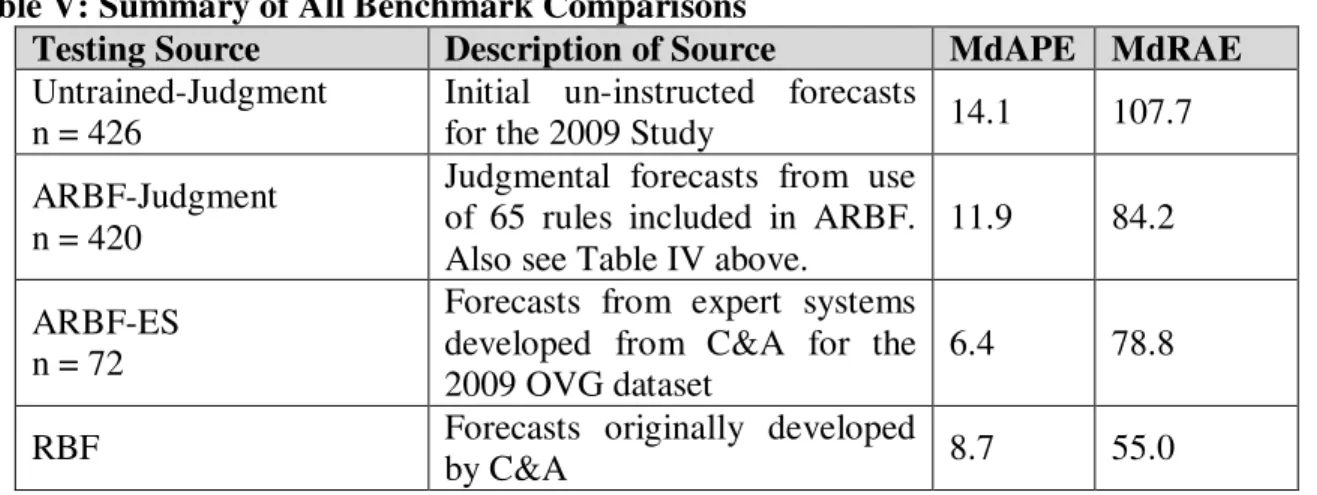
Next, to address the representativeness and generalizability of the principal result shown above, outcomes from the three benchmark comparisons discussed earlier are presented in Table V.
ReferTable V
H1Validation Untrained Validity Test: The test for MdAPE and MdRAE for the ARBF-Judgment
[11.9% and 84.2%] against the Untrained Judgment [14.1% and 107.7%] shows statistically significant differences with test p-values of < 0.02 and <0.0001 respectively. This provides confirmatory support for H1Validation, i.e. given any sort of rule-driven training, even with the
extensive 65 rule set and 18 features of time series, application of forecasting rules effectively supports judgmental processes, resulting in improved forecast accuracy.
H2Validation ARBF Expert System Validity Test: In comparing accuracy between judgmental
application of ARBF rules and expert-system driven forecasts for the same series, MdAPE and MdRAE yielded outcomes with ARBF-ES [6.4% and 78.8%] and ARBF-Judgment [11.9% and 84.2%]. The directional one-tailed p-values were > 0.5 for both MdAPE and MdRAE confirm that expert system driven forecasts, ARBF-ES, were not less accurate than those derived from ARBF-Judgment. This provides confirmatory support for H2Validation.
H3ValidationRBF: Here we used the forecasting expertise and 99 rules as reported in the original
1017 results from all judgmental groups - the coreRBF-Judgment group, ARBF-Judgment group, and
Untrained Judgment group. Results indicate that the above three experimental comparisons are different in the expected direction - i.e., C&A’s results using all the 99 rules from the rule set are better with p-values <0.0001 for all the contrasts. This provides confirmatory support for
H3Validation.
General Summary: In all three instances of the validation hypotheses, the results are consistent with the a priori expectations about the benchmarked validations. These results can then be argued as follows: all RBF results, including ARBF and coreRBF, produced judgmentally by the participants: (a) benefitted from rule-based training, (b) did not outperform the expert system benchmarks, and (c), were outperformed by forecasting expertise presented in the original RBF model (C&A). Findings from these validating hypotheses, then, clearly argue that the coreRBF-Judgment results were as expected and, therefore, by logical extension, suggest that some underlying processes offset the breadth of knowledge captured in the larger ARBF rule-set with the ease of application of the smaller coreRBF rules. This is evidenced by the lack of meaningful statistical differences in the forecasting accuracies between ARBF-Judgment and coreRBF-Judgment forecasts.
The important exploratory outcome to consider is that, for non-experts the coreRBF model is much simpler to communicate, understand, and learn. In particular, the IF…THEN… structure of the rules aligns with human reasoning processes and is easier to apply to judgmental forecasting tasks. With increasing expertise, forecasters may gradually transition to using a greater set of rules which, when applied systematically, will enhance the quality of the forecasting task beyond what coreRBF can deliver. As such, coreRBF is a good initial introduction to the dynamic concepts captured in the more extensive RBF model.
VI. Discussion of Results and Implications
Experts and derived expert systems were expected to be better at judgmental forecasting because they benefit from a fuller application of expert rules and are not limited by situational human processing and biases. Considering this, our findings for the validating hypotheses are as expected. However, expert systems can also be effective in informing judgmental forecasting considering the extensive knowledge inherently captured. As such, we demonstrate that even with a smaller, but essential, rule-set judgmental forecasting outcomes for non-experts can be improved.
Specifically, for the principal hypothesis, forecasting outcomes from use of ARBF and coreRBF rules were not different, most likely, due to the human information processing (HIP) limitations and trade-offs addressed earlier. The HIP literature suggests that decision makers in a complex decision milieu are bound to make mistakes. The longer decision makers must concentrate the worse their decisions usually become. Extending these findings to the process of forecasting examined here, (1) the probability of making an error of application per rule will probably be lower during the first few rules than during the last several rules in the rule set, and (2) in identifying errors of application during rule assessment, the ability to find errors will be much higher across 12 rules as opposed to 65. In our study, participants using ARBF might already be doing what we did for them during the experiment i.e. selectively apply some of the rules while leaving others out. By filtering out reduced rules based on forecasting expertise and prior validations, we minimized the potential for adhoc application of rules and promote, instead, the use of expert-derived rules.
1018 As coreRBF requires less time, results comparing ARBF and coreRBF suggest that there is little risk in using the coreRBF model to inform judgmental forecasting as compared to ARBF or, for that matter, compared to the 99 rules from RBF. Those working on forecasting tasks using ARBF almost exclusively required more time than did those using coreRBF. For example, from observations of task execution in the computer lab, when using the ARBF model, all participants required time in the afternoon session to complete the task whereas, when using coreRBF, most participants completed their task in the morning session. Only in one case did a student who was assigned the coreRBF model need additional time in the afternoon session. Furthermore, participants rarely had questions about the execution procedure when using coreRBF; almost all questions came from participants during application of ARBF. These were usually procedural or related to interpretation of rules and features. These differences in temporal needs are anecdotal evidence that using the coreRBF model for training and pedagogy would permit greater efficiency in producing judgmental forecasts.
In a pragmatic forecasting context, where an expert system for forecasting may not always be available and forecasting needs are driven by organizational needs for efficiency, use of coreRBF would certainly economize on time. Similarly, for purposes of pedagogy, using coreRBF as part of a forecasting course or as a topic treated in finance, production and supply chain coursescan reduce the instructional time necessary for imparting necessary forecasting knowledge. Furthermore, coreRBF as a modeling system would open the content to introducing other critical forecasting issues such as forecaster adjustment behaviors and development of forecasting support systems.
The simple rules generated as part of this rule reduction can be effectively embedded within existing forecasting systems to provide enhanced support to non-experts. From feature-based detection and adjustment to application of simple rules, coreRBF is amenable to simple integration within forecasting decision support systems (Adya and Lusk, 2012).47
The reduced set of coreRBF rules is by no means the final note in this dynamic and important area of research and pedagogy. In identifying the essential 12 rules, we relied on several decades of empirical evidence and significant forecasting expertise. As the 12 rules had already been validated and calibrated originally in C&A, this study focused largely on identifying and verifying that these core rules were beneficial to the forecasting process and could be pragmatically applied to judgmental tasks without degrading accuracy. Evidence developed from extensive human subject studies presented in this paper confirms this. We, however, hope that future research in this direction, especially studies using design science or artificial intelligence approaches, would apply other approaches to identifying a more effective set of rules that might improve upon coreRBF.
47
All the instructional materials used in delivering the coreRBF course are available from the authors; we waive all intellectual property rights to the academic—i.e., non-commercial, use of this material.
1019
References
Adya, M., 2000, Corrections to rule-based forecasting: findings from a replication, International Journal of Forecasting 16, 125-127.
Adya, M., F. Collopy, J.S. Armstrong, and M. Kennedy, 2000, An application of rule-based forecasting to a situation lacking domain knowledge, International Journal of Forecasting 16, 477-484.
Adya, M., F. Collopy, J.S. Armstrong, and M. Kennedy, 2001, Automatic identification of time series features for rule-based forecasting, International Journal of Forecasting 17, 143-157. Adya, M. and E.J. Lusk, 2012, Designing effective forecasting Decision Support Systems:
Aligning task complexity and technology support, in C. Jao, ed.: Decision Support Systems, ISBN: 978-953-51-0799-6, (InTech, DOI: 10.5772/51255). Available from:
http://www.intechopen.com/books/decision-support-systems_2012/designing-effective-forecasting-decision-support-systems-aligning-task-complexity-and-technology-sup
Adya, M., E.J. Lusk, and M. Balhadjali, 2009, Decomposition as a complex skill acquisition strategy in management education: A case study in business forecasting, Decision Sciences Journal of Innovative Education 7, 9 - 36.
Angeli, C., 2010, Diagnostic expert systems: From expert’s knowledge to real-time systems, in P. S. Sajja and R. Akerkar, eds.: Advanced Knowledge Based Systems: Model, Applications, & Research (TMRF e-Books)Vol. 1, pp. 50-73.
Armstrong, J.S., and F. Collopy, 1993, Causal forces: Structuring knowledge for time series extrapolation, Journal of Forecasting 12, 103-115.
Armstrong, J.S., and F. Collopy, 1992, Error measures for generalizing about forecasting methods: Empirical comparisons, International Journal of Forecasting 8, 69-80.
Chang, C-L., J-A. Jimenez-Martin, M. McAleer, and T.P. Amaral, 2013, The rise and fall of S&P500 variance futures, North American Journal of Economics and Finance 25, 151-167. Clancey, W.J., 1983, The epistemology of a rule-based expert system: A framework for
explanation, Artificial Intelligence 20, 215-251.
Clemens, R.T., 1989, Combining forecasts: A review and annotated bibliography, International Journal of Forecasting 5, 559-583.
Collopy, F., and J.S. Armstrong, 1992, Rule-based forecasting: Development and validation of an expert systems approach to combining time series extrapolations, Management Science 38, 1394-1414.
Cowan, N., 1988, Evolving conceptions of memory storage, selective attention, and their mutual constraints within the human infromation processing system, Psychological Bulletin 104, 163-191.
Hanke, J., D. Wichern, and A. Reitsch, 2001, Business Forecasting, Seventh Edition: (ISBN: 0-13-087810-3, Prentice Hall International).
Kalinga J., R. Lonseth, and A.A. Lonseth, 2013, Bottom-up approach for productivity measurement and improvement, International Journal of Productivity and Performance Management 62, 387-406.
Kim, T., J. Hong, and H. Koo, 2013, Forecasting diffusion of innovative technology at pre-launch, Industrial Management + Data Systems 113, 800-816.
Korol, T., 2013, Early warning models against bankruptcy risk for central european and Latin American enterprises, Economic Modelling 31, 22-35.
1020 Makridakis, S., A. Andersen, R. Carbone, R. Fildes, M. Hibon, R. Lewandowski, J. Newton, E. Parzen, and R. Winkler, 1982, The accuracy of extrapolation (time series) methods: Results of a forecasting competition, International Journal of Forecasting 1, 111-153. Makridakis, S., and M. Hibon, 2000, The M-3 Competition results: Conclusions and
implications, International Journal of Forecasting 16, 451-476.
Mohammad S.M., M. Anvari, and M. Saberi, M. (2103) Targeting performance measures based on performance prediction, International Journal of Productivity and Performance Management 61, 46-68.
Sanders, N.R., and L.P. Ritzman, 1992, The need for contextual and technical knowledge in judgmental forecasting, Journal of Behavioral Decision Making 5, 39 – 52.
O'Connor, M., W. Remus, and K. Griggs, 1993, Judgmental forecasting in times of change, International Journal of Forecasting 9, 163-172.
Ramsey, C.L., J.A. Reggia, D.S. Nau, and A. Ferrentino, 1986, A comparative analysis of methods for expert systems, International Journal of Man-Machine Studies 24, 475-499. Sall, J., A. Lehman, and L. Creighton, 2001, JMP Start Statistics, Second Edition,(ISBN
0-534-35976-1: Duxbury Press International).
Simon, H., 1980, Cognitive science: The newest science of the artificial, Cognitive Science, 4, 33 – 46.
Shanteau, J., and T.R. Stewart, 1992, Why study expert decision making? Some historical perspectives and comments, Organizational Behavior and Human Decision Processes, 53, 95 – 106.
Shukla, M., and S. Jharkharia, 2013, Agri-fresh produce supply chain management: A state-of-the-art literature review, International Journal of Operations & Production Management 33, 114-158.
Tiacci, L., and S. Saetta, 2012, Demand forecasting, lot sizing and scheduling on a rolling horizon basis, International Journal of Production Economics 140, 803-818.
1021
Appendix – The Reduced Rule-Set
In this presentation we maintained the Rule Numbering that is found in C&A. Short Model Level
Rule 29: Level Discontinuities (Short Model Level)
IF there is a level discontinuity, i.e., sort of a step change, in the series, THEN add 0.10 to the weight on the Random Walk and subtract it from the weight of the Holt Model.
Rule 32: Changing Recent Trends (Short Model Level)
IF there is an unstable recent Trend, THEN add 0.45 to the weight on Random Walk model and subtract 0.15 from the Linear Regression Weigh and subtract 0.30 from the Holt Model Weight.
Short Model Trend
Rule 40: Causal Forces Unknown (Short Model Trend)
IF the causal forces are unknown, THEN add 0.05 to the weight on the Random Walk and subtract it from that on the Linear regression trend estimate.
Rule 41: Dissonance (Short Model Trend)
IF the direction of the recent trend and the direction of the basic trend are not the same, OR if the trends agree with one another but differ from the causal forces, THEN add 0.15 to the weight on the Random Walk and subtract 0.05 from the Linear regression and 0.10 from the Holt Model Weight.
Rule 42: Inconsistent Trends (Short Model Trend)
IF the direction of the basic trend and the direction of the recent trend are not the same, AND the basic trend is not changing, THEN add 0.20 to the weight on the Linear regression trend and subtract it from Holt Model trend weight.
Long Model Level
Rule 67: Level Discontinuities (Long Model Level)
IF there is a level discontinuity, THEN add 0.10 to the weight on the Random Walk and subtract it from the level weight of the Holt Model.
Rule 71: Changing Recent Trends (Long Model Level)
IF there is an unstable recent trend, THEN add 0.63 to the level weight of the Random Walk and subtract 0.21 from the Linear regression Level Weigh and subtract 0.42 from the Holt Model Level Weight.
Long Model Trend
Rule 76: Causal Forces Unknown (Long Model Trend)
IF the causal forces are unknown, THEN add 0.10 to the weight on the Random Walk Model’s Trend and subtract it from that on the Linear regression trend estimate.
Rule 77: Dissonance (Long model Trend)
IF the direction of the recent trend and the direction of the basic trend are not the same, OR if the trends agree with one another but differ from the casual forces, THEN add 0.15 to the trend weight on the Random Walk and subtract 0.05 from the Linear Regression and 0.10 from the Holt Model Weight.
Rule 78: Inconsistent Trends (Long model Trend)
IF the direction of the basic trend and the direction of the recent trend are not the same AND the Basic trend is not changing, THEN add 0.10 to the weight of the Linear regression trend and subtract it from the Holt Model.
1022
Rule 86: Inconsistent Trends (Long model Trend)
IF the directions of the recent and basic trends are not the same, THEN subtract 0.10 from the weight on Linear regression and add 0.033 to the Weight on the Holt model and 0.067 to the weight on the Random Walk Model.
Rule 87: Changing Basic Trend (Long model Trend)
IF there is a changing basic trend, THEN add 0.24 to the Random Walk Trend weight and 0.06 to the Holt Model’s Trend weight and subtract 0.30 from the Linear regression’s Trend weight.
Final Blending of the Short and the Long Models
Just as we did in the Full Model Rule version, after you make the weight adjustments, then you will select the BLENDING Rule from the Four BLENDING options given in Rules 96 to 99 as found in the Full Rules document.
This blending of the Short and the Long Model then gives finally the Rule Based Forecasts just as it did for the Full Rule Set. So here you see that the only difference between the two systems: Full and Reduced Rules, is the number of weighting rules used to modify the initial weights from the Four Components.
It may be instructive at this point to provide a brief illustration of the scoring system that is used to create the coreRBF models used to create the forecasts.
We will use, for illustration, the Short Model Level [SML]. First assuming that we have prepared the data as indicated above and that we will be using untransformed data—i.e., measured actual realizations; given this assume that we have measured the following Level values:
Random Walk = 24,980; Regression Level = 32,874; Holt Level = 28,002
Next we modify the initially the C&A weights from Table II that are used to fix the Short Model Level [SML]. The initial weights from Table II are:
40% of the Random Walk; 20% of the Linear Regression Level; 40% of the Holt Level.
There are only two rules that pertain to fixing the SML: Rule 29 and Rule 32. Assume there is a Level Discontinuity for the time series under examination. In this case onlyRule 29 is activated:
Rule 29: Level Discontinuities (Short Model Level)
IF there is a level discontinuity, i.e., sort of a step change, in the series, THEN add 0.10 to the weight on the Random Walk and subtract it from the weight of the Holt Model.
Rule 29 thus indicates that we should modify the initial starting weights as follows: 50% [40% ++++ 10%] of the Random Walk
20% of the Linear Regression Level [Unchanged by Rule 29] 30% [40% −−−− 10%] of the Holt Level.
This means that the Short Model Level [SML] used in the coreRBF model will be: SML = 27,465.40 [50% × 24,980 + 20% × 32,874 + 30% × 28,002]
Similar computations are made for the other three parameters the SMTrend, the LMLevel and LMTrend.
1023
Table I: Time Series Features Used in This Study
Feature Description [From C&A(1992)]
Level discontinuity or Level shift
Dramatic and significant changes in the level of the series (steps)
Causal forces The net directional effect of the principal factors acting on the series. Growth exerts an upward force. Decay
exerts a downward force. Supporting forces push in the direction of the historical trend. Opposing forces work against the trend. Regressing forces work towards a mean. When uncertain, forces should be unknown. Direction of basic trend Direction of trend after fitting linear regression to past
data.
Direction of recent trend The direction of trend that results from fitting Holt’s exponential smoothing to past data.
Changing basic and recent trends
Underlying trend that is changing over the long run. Irrelevant early data Early portion of the series results from a substantially
different underlying process.
Outliers Isolated observation from a 2 standard deviation band of linear regression
Table II: Initial Weights Recommended by C&A Starting Weights for Short
and Long Models from C&A Random Walk Linear Regression Holt’s ES
Short Model Level 0.40 0.20 0.40 Short Model Trend 0.40 0.20 0.40 Long Model Level 0.33 0.33 0.34 Long Model Trend 0.00 0.60 0.40
Table III: Evidence on Order Effects between ARBF and coreRBF Forecasts
Testing Source Description of Source MdAPE MdRAE
ARBF1 n = 192
ARBF forecasts for 2009 group that used ARBF forecasts first and then used coreRBF [matched with coreRBF2]
12.0 86.8 ARBF2
n = 228
ARBF forecasts for 2009 group that used coreRBF forecasts first and then used ARBF [matched with coreRBF1]
11.8 82.6 coreRBF1
n = 228
coreRBF forecasts for 2009 group that used coreRBF forecasts first and then used ARBF [matched with ARBF2]
11.0 91.3 coreRBF2
n = 192
coreRBF forecasts for 2009 group that used ARBF first and then used coreRBF [matched with ARBF1]
1024
Table IV Test of the Principal Hypothesis
Forecast Model MdAPE MdRAE
ARBF-Judgment,
n =420 11.9 84.2 coreRBF-Judgment,
n =420 11.7 87.7 Two Tailed p-values 0.89 0.33
Table V: Summary of All Benchmark Comparisons
Testing Source Description of Source MdAPE MdRAE
Untrained-Judgment n = 426
Initial un-instructed forecasts
for the 2009 Study 14.1 107.7 ARBF-Judgment
n = 420
Judgmental forecasts from use of 65 rules included in ARBF. Also see Table IV above.
11.9 84.2 ARBF-ES
n = 72
Forecasts from expert systems developed from C&A for the 2009 OVG dataset
6.4 78.8 RBF Forecasts originally developed