Theses & Dissertations Boston University Theses & Dissertations
2019
Three essays on quantile factor
analysis
https://hdl.handle.net/2144/34896
GRADUATE SCHOOL OF ARTS AND SCIENCES
Dissertation
THREE ESSAYS ON QUANTILE FACTOR ANALYSIS
by
ANDR´
ES G. SAGNER
B.A. (Industrial Engineering), Federico Santa Maria University, 2004
M.A. (Economics), University of Chile, 2009
Submitted in partial fulfillment of the
requirements for the degree of
Doctor of Philosophy
2019
First Reader
Zhongjun Qu, Ph.D.
Associate Professor of Economics
Second Reader
Pierre Perron, Ph.D. Professor of Economics
Third Reader
Iv´an Fern´andez-Val, Ph.D. Professor of Economics
It has been a long journey. Looking back in time, I realize that this adventure would not have been possible without the help and support of a long list of people, to whom I am most grateful. First and foremost, I want to thank my parents, Carlos and Silvia, for providing me a good education. Both of you are a big part of who I am today, and I thank you so much for all your love and support from away at different stages of this adventure.
I am very grateful to Rodrigo Alfaro, Roberto Alvarez, Dalibor Eterovic and Jaime Ruiz-Tagle for writing recommendation letters and helping me in finding my way to BU. I had the pleasure not only to work with all of you but also to learn from you and your professional experience, in different time periods, at the Central Bank of Chile and the University of Chile. A special thank you is due to Rodrigo for encouraging me and believing that I was capable of undertaking the challenge of a Ph.D. in Economics program. More than a mentor or a boss, I consider you a friend.
I would also like to acknowledge the financial support of the Central Bank of Chile and the Ministry of Education of Chile through their Becas de Doctorado en el Extranjero Becas Chile program. The financial aid granted by these institutions considerably alleviated the pressure of sharing my time between looking for sources of funding and writing this dissertation. Their impact on my formation as an economist is invaluable.
I owe immense gratitude to my advisors Zhongjun Qu, Pierre Perron, and Iv´an Fern´andez-Val. I thank Zhongjun for showing interest in my preliminary idea and continuously guiding my work towards completing a well-structured, much more in-teresting and relevant dissertation than I initially thought. He is an excellent advisor and incredibly generous with his knowledge. I am grateful to Pierre for always having interesting and brilliant comments and suggestions when I presented different stages
a professor and advisor. I thank Iv´an for always having the precise advice when I was stuck at a technical aspect of the dissertation. His recommendations were always a balanced combination between being technically rigorous and avoiding intricated arguments. Having them as advisors was an extraordinary experience and I look forward to continue learning from them in the future.
I am grateful to my colleagues and friends Jon Hersh, Lolo Palacios, Mario Cruz, Nick Saponara, Hannah Ye and Alexis Montecinos for sharing my time at BU with you. You all helped make these years in Boston much more pleasant and entertaining. A special thanks to Mirko Fillbrunn and Andre Mittag for allowing me to stay at your apartment at the very final stage of this project.
Last but not least, I am deeply grateful to my beloved wife Claudia and my beloved son Federico. Thank you for all your love, support, patience and goodness during the writing of this dissertation and when I sometimes thought I would not be able to complete it; both of you are the heart of this adventure. You believed in me, and I will always love you for that. This thesis is dedicated to you.
ANDR´
ES G. SAGNER
Boston University, Graduate School of Arts and Sciences, 2019
Major Professor: Zhongjun Qu, Ph.D.
Associate Professor of Economics
ABSTRACT
In the first chapter of this dissertation, I develop a method that extends quan-tile regressions to high dimensional factor analysis. In this context, the conditional quantile function of a panel of variables is endowed with a factor structure. Thus, both factors and factor loadings are allowed to be quantile-specific. I provide a set of conditions under which these objects are identified, and I propose a simple two-step iterative procedure called Quantile Principal Components (QPC) to estimate them. Uniform consistency of the estimators is established under general assumptions when both the cross-section and time dimensions (N and T, respectively) become large jointly.
In the second chapter, I propose a novel measure to quantify systemic risk from the information contained in asset returns. In the context of the external habits for-mation model of Campbell and Cochrane (1999) and heteroskedastic stock returns, I show that the equilibrium risk premium has a factor structure where factors are a monotonic transformation of the systemic risk variable in the structural model, and one of the factors affects the variance of excess returns. I estimate the factor model using the QPC estimation procedure. Simulations of the model calibrated to the US show a good performance of the proposed metric computed at quantiles differ-ent than the median. When estimated using post-war data, the proposed measure
market turbulence periods; and it can forecast extreme tight and loose financial con-ditions, and sharp shifts in both economic activity and industrial production up to one year ahead.
The third chapter provides limiting distributions of the QPC estimators proposed in the first chapter. Under certain additional assumptions related to the density of the observations about the quantile of interest, and the relationship between N and
T, I show that the QPC estimators are asymptotically normal with convergence rates similar to the ones derived in the traditional factor analysis literature. Monte Carlo simulations suggest that the proposed theory provides a good approximation to the finite sample distribution of the QPC estimates.
1 High Dimensional Quantile Factor Analysis 1
1.1 Introduction . . . 1
1.2 Model and Estimation . . . 4
1.2.1 The Model . . . 4
1.2.2 Identification . . . 8
1.2.3 The QPC Estimator . . . 13
1.3 Consistency of the QPC Estimator . . . 22
1.4 Conclusions . . . 27
2 Measuring Systemic Risk: A Quantile Factor Analysis Approach 36 2.1 Introduction . . . 36
2.2 Model . . . 41
2.2.1 An External-Habit-Based Asset Pricing Model . . . 42
2.2.2 Measure of Systemic Risk of Simulated Data . . . 46
2.3 Systemic Risk Measure for the US . . . 56
2.3.1 Data and Estimation . . . 56
2.3.2 In-Sample Properties . . . 59
2.3.3 Early-Warning Indicator Properties . . . 61
2.4 Conclusions . . . 65
3 Limiting Distributions for High Dimensional Quantile Factor Anal-ysis 78 3.1 Introduction . . . 78
3.2.1 Limiting Distributions . . . 80
3.2.2 Estimation of Asymptotic Variance-Covariance Matrices . . . 86
3.2.3 Monte Carlo Simulations . . . 89
3.3 Conclusions . . . 92
Appendices 102 A High Dimensional Quantile Factor Analysis 103 A.1 Proof of Proposition 1.2.1 . . . 103
A.2 Proof of Theorem 1.2.1 . . . 105
A.3 Proof of Theorem 1.3.1 . . . 110
B Measuring Systemic Risk: A Quantile Factor Analysis Approach 118 B.1 Optimality Conditions of the Model . . . 118
B.2 Proof of Proposition 2.2.1 . . . 120
B.3 Data Description . . . 123
B.3.1 Calibration . . . 123
B.3.2 Measure of Systemic Risk for the US . . . 124
C Limiting Distributions for High Dimensional Quantile Factor Anal-ysis 127 C.1 Proof of Theorem 3.2.1 . . . 127 C.2 Proof of Theorem 3.2.2 . . . 132 References 134 Curriculum Vitae 143 x
1.1 Correlation Between Estimated and True Parameters - DGP 1 . . . . 33
1.2 Correlation Between Estimated and True Parameters - DGP 2 . . . . 34
1.3 Correlation Between Estimated and True Parameters - DGP 3 . . . . 35
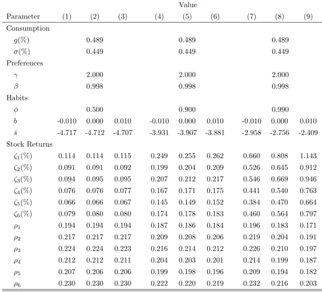
2.1 Calibrated Parameters . . . 72
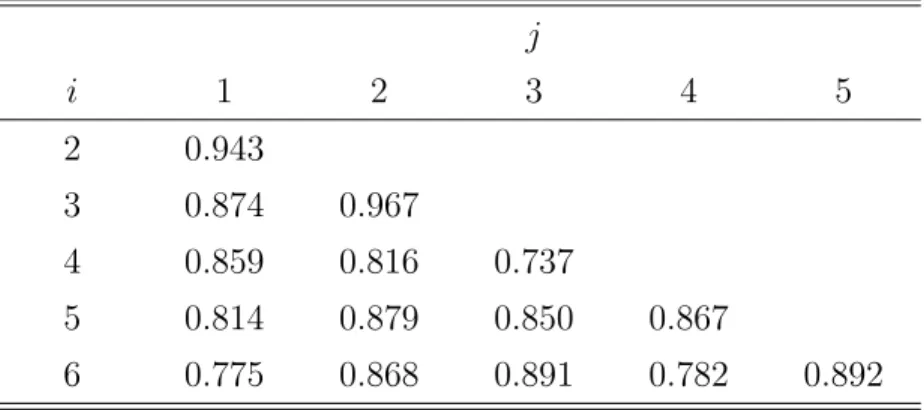
2.2 Correlation Between Stock Returns (ωij) . . . 73
2.3 Average Correlation Between Simulated and Estimated st . . . 74
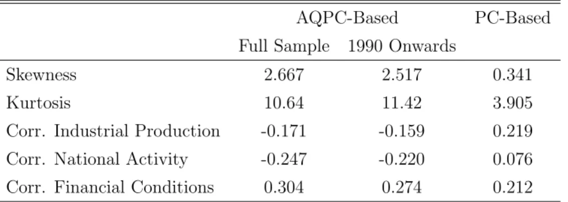
2.4 Systemic Risk Measures Summary Statistics . . . 75
2.5 Forecast Performance - AQPC v/s Unconditional Quantiles . . . 76
2.6 Forecast Performance - AQPC v/s PC . . . 77
3.1 Mean of Standardized QPC Estimators . . . 100
3.2 Standard Deviation of Standardized QPC Estimators . . . 101
1·1 Performance of QPC and PC Estimators ofβt - DGP 1 . . . 29
1·2 Performance of QPC and PC Estimators ofβt - DGP 2 . . . 30
1·3 Performance of QPC Estimators of γt - DGP 2 . . . 31
1·4 Performance of QPC and PC Estimators ofβt - DGP 3 . . . 32
2·1 Samples Characterization . . . 67
2·2 Risk-Free Rate Cyclicality . . . 68
2·3 Measure of Systemic Risk for the US . . . 69
2·4 Comparison of Systemic Risk Measures for the US . . . 70
2·5 Adverse Shocks Forecast . . . 71
3·1 Histogram of QPC Factors (T = 50) . . . 94
3·2 Histogram of QPC Factors (T = 100) . . . 95
3·3 Histogram of QPC Factor Loadings (T = 50) . . . 96
3·4 Histogram of QPC Factor Loadings (T = 100) . . . 97
3·5 Histogram of QPC Common Components (T = 50) . . . 98
3·6 Histogram of QPC Common Components (T = 100) . . . 99
AMEX . . . American Express
APC . . . Adjusted principal components
AQPC . . . Adjusted quantile principal components BEA . . . Bureau of Economic Analysis
CPI . . . Consumer price index
CRSP . . . Center for Research on Security Prices DGP . . . Data generating process
iid . . . Independent and identically distributed MLE . . . Maximum likelihood estimation
NASDAQ . . . National Association of Securities Dealers Automated Quotation
NBER . . . National Bureau of Economic Research NYSE . . . New York Stock Exchange
OLS . . . Ordinary least squares PC . . . Principal components QFA . . . Quantile factor analysis
QPC . . . Quantile principal components S&P 500 . . . Standard & Poor’s 500 index US . . . United States
VAR . . . Vector autorregresion
a→b . . . a is close, but not equal, to b a⇒b . . . a implies b Op(·) . . . Bounded in probability d → . . . Convergence in distribution p →, op(·) . . . Convergence in probability
CORR[a, b] . . . Correlation betweena and b
k·k . . . Euclidean norm
Im . . . Identity matrix of size m
1{·} . . . Indicator function
N(a, b) . . . Normal distribution with parametersa and b O(·) . . . Order of approximation
U(a, b) . . . Uniform distribution with parameters a and b
Chapter 1
High Dimensional Quantile Factor
Analysis
1.1
Introduction
During the last decades, high dimensional factor analysis has become an increasingly popular and useful statistical tool in a large number of economic applications. Its popularity resides in the fact that it is a practical and easy way to summarize the information contained in large data sets into a small number of reference, unobserved variables that jointly describe a mean curve. For instance, factor analysis has been used to model asset returns as a function of a small number of risk factors (Ross, 1976; Connor and Korajczyk, 1988); decompose the business cycle into common and specific shocks at the cross-country level (Gregory and Head, 1999; Forni et al., 2000; Crucini et al., 2011; Karadimitropoulou and Leon-Ledesma, 2013), national level (Stock and Watson, 1989; Mariano and Marasawa, 2003; Aruoba et al., 2009), and industry-level (Forni and Reichlin, 1998); improve forecasting models by including the so-called diffusion indexes (Stock and Watson, 1999, 2002); and construct measures of systemic risk (Kritzman et al., 2011), macroeconomic or financial uncertainty (Jurado et al., 2015) and network connectedness (Billio et al., 2012) which are key for policy makers to perform macro and financial stability monitoring; among many other applications. In this chapter, I extend the quantile regression approach popularized by Koenker and Bassett (1978) to high dimensional factor analysis. I name this concept high
dimensional quantile factor analysis (QFA). In this setup, for any τ ∈ (0,1), the τ -th quantile function of a panel containing N variables yit observed along T periods conditional on λ0i(τ) and ft0(τ), Qyit(τ|λ
0
i(τ), ft0(τ)), where both N and T are large, is a linear function of K(τ)<min{N, T} unobserved quantile-specific factors f0
t (τ) that capture the common variation of all variables at each period t. Moreover, the number of quantile-specific factors,K(τ), and the sensitivity or factor loading of each variableito each quantile factor,λ0
i (τ), are also permitted to be quantile-specific. In this manner, the proposed setup captures the idea of aquantile factor model which has the particularity of being flexible enough to characterize several linear and nonlinear factor models available in the related literature.
Under standard assumptions, I show that both the quantile factors f0
t (τ) and the quantile factor loadings λ0i (τ) are individually identified. The type of identification depends crucially on the rotation chosen by the econometrician. In particular, the identification of f0
t (τ) and λ0i (τ) is local if an orthogonal rotation, extensively used in Principal Components (PC), or a recursive-type rotation is considered, whereas it is global once an errors-in-variables-type rotation is employed. However, the identi-fication of the quantile common component c0
it(τ) = λ0i (τ)
0 f0
t (τ) is always a global one. Moreover, I show that if the ordering of the observable variables yit is known in advance i.e., we know which variable is affected by which quantile factor, then all previous rotations deliver quantile common components that are observationally equivalent.
I propose a simple two-step iterative procedure based on the minimization of the quantile loss function to obtain theQuantile Principal Components (QPC) estimator of ft0(τ) and λi0(τ) for any τ ∈(0,1). In the first step, the estimator of the quantile factors, ˆft(τ), is computed using quantile regressions across cross-sections for each t, where the unobserved quantile loadings are replaced by an initial guess. Then, in the
second step, the estimator of the quantile factor loadings, ˆλi(τ), is computed using quantile regressions across time periods for each i, given the previous estimates for the quantile factors. This estimation procedure offers some advantages in terms of efficiency, compared to the principal components methodology, especially in nonlinear setups or in factor models where factors have impacts over higher moments of the observable variable yit.
In addition, I establish the uniform consistency of both ˆft(τ) and ˆλi(τ) under general assumptions. In the proof, I proceed as in Chen et al. (2014) and show first the uniform consistency of the QPC estimator of the quantile common component as N, T → ∞ jointly, in view of the fact that the objective function involved in the minimization of the quantile loss function is convex in terms of the estimator of the quantile common component, ˆcit(τ) ≡ λˆi(τ)0fˆt(τ). This feature, together with the compactness of the parameter set, allows me to invoke a standard uniform law of large numbers argument. Then, given this intermediate result, uniform consistency of ˆft(τ) and ˆλi(τ) follows from the assumptions imposing a strong factor structure.
This work is related to the relatively recent literature on panel data models where the error component contains interactive effects (or equivalently, a factor structure), e.g. Koenker (2004), Pesaran (2006), Bai (2009), Kato et al. (2012), Bai and Li (2014), Harding and Lamarche (2014), Moon and Weidner (2015, 2017), Fernandez-Val and Weidner (2016), among others. Albeit its similarity with this setting, these models differ from quantile factor models in at least two key aspects. First, in the QFA context, the regressors of the model are the factors which, besides being quantile-specific, are not observable by the econometrician, entailing in this manner several estimation challenges. So, this chapter contributes to the literature by providing an estimation methodology that is easy to implement even in nonlinear environments. Second, in most of these models, the unobserved individual and time heterogeneity is
treated as nuisance parameters. In consequence, a large part of the analysis is devoted to the properties of the fixed or random effects estimator, while the properties of the factors and the factor loadings are barely explored. I contribute to this strand of the related literature by analyzing the asymptotic properties of these objects in a high dimensional quantile framework.
The rest of the chapter is organized as follows. Section 1.2 starts by presenting the statistical model behind high dimensional QFA and provides some examples to illustrate this concept. Section 1.2.2 discusses in detail the individual identification of the quantile factors and quantile factor loadings, while Section 1.2.3 presents the iterative procedure to obtain their QPC estimators and highlights some of their prop-erties. Section 1.3 provides the set of assumptions required to establish the uniform consistency of the QPC estimator. Finally, Section 1.4 concludes and suggests further steps for future research on this topic. All proofs of main and intermediate results are given in Appendix A.
1.2
Model and Estimation
In this section, I present the data generating process behind high dimensional quantile factor analysis. I provide next a set of conditions under which the relevant parameters of the model are identified by the data. Finally, I propose an iterative algorithm to estimate the quantile-specific factors and factor loadings and I discuss in detail some of its properties.
1.2.1 The Model
The main idea behind traditional factor analysis is that the behavior across T time periods of a set of N observed random variables can be characterized by a linear
combination of K <min{N, T}factors plus an error term. Formally, yit=λ0i0f 0 t +e 0 it
where yit is the i-th observed random variable at time t, ft0 is a vector containing K factors, λ0
i is a vector of factor loadings or sensitivities of the i-th variable to each factor, e0
it is an iid error term, and the superscript “0” stands for true or population parameters. The product c0it ≡ λ0i0ft0 is typically known as the common component
of yit, whereas the error term is sometimes called the idiosyncratic component. In addition, the theory underlying high dimensional factor analysis allows both N and
T to be large, and it assumes that the number of factors K is known1. Finally, note that all elements on the right-hand side of the above equation are not observable by the econometrician.
In this chapter, I extend the traditional high dimensional factor analysis model by allowing the factors or the factor loadings, or both, to be a function of a random variable uit distributed uniformly over the [0,1] interval. To be precise, I consider that the observable variable yit is generated by the following data generating process
yit =λ0i(uit)0ft0(uit), uit ∼ U(0,1) (1.1)
Assumption 1.2.1. For all i, t and τ ∈ (0,1), the common component c0
it(τ) ≡ λ0 i(τ) 0f0 t(τ) is nondecreasing in τ. Let τ ∈ (0,1) and G(·|θ0
it(τ)) be the cumulative distribution function of yit conditional on θ0it(τ) ≡ [λ0i(τ)0, ft0(τ)0]0. Under Assumption 1.2.1, the τ-th condi-tional quantile function of the observable variable yit given θit0(τ), Qyit(τ|θ
0
it(τ)) ≡
1If this assumption is relaxed, thenKcan be consistently estimated from the data by using the
information-criteria-based tests proposed by Bai and Ng (2002), or the testing procedure presented in Onatski (2009), Kapetanios (2010), and Ahn and Horenstein (2013).
inf{yit:G(yit|θit0(τ))≥τ}, is given by Qyit τ|θ 0 it(τ) =λ0i (τ)0ft0(τ), τ ∈(0,1) (1.2) where the number of factors, K(τ), is also allowed to be quantile-specific. In other words, the above equation says that all conditional quantiles of the observable random variableyit have a factor model structure. So, equation (1.1) summarizes the idea of a
quantile factor analysis model and, consequently, we can refer to ft0(τ) andλ0i (τ) in equation (1.2) as quantile factors and quantile factor loadings, respectively. At first glance, the linearity of the proposed framework may seem restrictive. However, as will see in the next examples, equation (1.1) has the potential to nest several nonlinear factor model structures.
Example 1 (Standard Factor Model). Let yit =α0iβt0+vit0, where both α0i and
β0
t are scalars and v0it is an iid random variable with cumulative distribution function
Gv(·). By defining vit0 ≡ G
−1
v (uit) where uit ∼ U(0,1) for all i,t, the standard factor model can be rewritten in the form of (1.1) by setting λ0i (uit) = [α0i,1]0 and
ft0(uit) = [βt0, Gv−1(uit)]0, or λ0i(uit) = [α0i, G−v1(uit)]0 and ft0(uit) = [βt0,1]0.
Example 2 (Location-scale Factor Model). Letyit =α0iβt0+γt0vit0, whereγt0 >0 for allt.Similar to the previous case, this model can be rewritten in the form of (1.1) by defining λ0 i (uit) = [α0i, G −1 v (uit)]0 and ft0(uit) = [βt0, γt0] 0, or λ0 i(uit) = [αi0,1] 0 and f0 t(uit) = [βt0, γt0G − v1(uit)]0, where vit0 ≡G −1
v (uit) with uit∼ U(0,1) for alli, t.
Example 3 (Non-linear Factor Model). Let yit = α0iβt0ev 0
it, where α0
i, βt0 > 0 for all i and t, respectively. If λ0
i (uit) = α0ieaG
−1
v (uit) and f0
t (uit) = βt0e(1
−a)G−v1(uit),
a∈[0,1], then this model has the form of (1.1).
The examples exhibited above are only a few out of many cases where a factor model structure can be represented by a QFA model.
Example 1 corresponds to the standard linear case where both the factors and the factor loadings affect only the mean of the observable variable, i.e. the homoskedastic case. Its configuration implies that only the factors (or the loadings) are quantile-specific and that one of the factor loadings (or factors) has to be equal to 1. This, in turn, implies that the quantile functions given by (1.2) are simply a vertical displace-ment of one another.
A somewhat more complicated case is considered in Example 2. In this context, the factors not only affect the mean of the observable variable but also its variance. Thus, the heteroskedasticity of this model is proportional to the square of γt0. More-over, two key aspects of this example are worth highlighting. First, Assumption 1.2.1 imposes an additional restriction to the domain of one of the factors (γ0
t >0), which suggests that equations (1.1) and (1.2) are not necessarily equivalent; the latter being the most restrictive one. Second, the number of factors depends indeed on τ. In particular, if the idiosyncratic componentv0
it is symmetric about the origin, then the conditional quantile function evaluated at the median is equal to 0 andft0(0.5) =βt0, i.e. K(0.5) = 1. On the contrary, for any τ 6= 0.5, the conditional quantile function is different from 0 and, consequently,f0
t (τ) = [βt0, γt0] and K(τ) = 2.
Finally, Example 3 is a nonlinear factor model describing the behavior of a strictly positive observable variable. The data generating process implies that either the factors or the factor loadings, or both, are quantile-specific. Lastly, note that logyit= logα0i+ logβt0+Gv−1(uit), that is, the factor model is linear for logyit so we can define ˜ λ0 i (uit) = [logα0i+aG −1 v (uit),1]0 and ˜ft0(uit) = [1,logft0+ (1−a)G −1 v (uit)],a∈[0,1], and the transformed model has the form of a quantile factor analysis model.
The matrix representation of equation (1.2) is given by
QY τ|θ0(τ)
where Y is a T ×N matrix of observable variables, F0(τ) = [f0
1 (τ), . . . , fT0(τ)]
0 ∈
ΘF ⊂RT×K(τ)is aT×K(τ) matrix of quantile factors, Λ0(τ) = [λ01(τ), . . . , λ0N(τ)]
0 ∈
ΘΛ ⊂ RN×K(τ) is a matrix of quantile factor loadings of dimension N ×K(τ), and
θ0(τ) ≡ [Λ0(τ)0, F0(τ)0]0. The T ×N matrix C0(τ) ≡ F0(τ) Λ0(τ)0 contains all the
common components of the model.
1.2.2 Identification
In this section, I provide a set of assumptions under which the population factor loadings and factors,θ0(τ), are identified by the data. I start by providing a definition of identification in this context.
Definition 1.2.1 (Identification). For all τ ∈(0,1), let θ(τ)≡[Λ(τ)0, F(τ)0]0 be a parameter matrix. We say that θ(τ) is identified at θ0(τ) ∈ΘΛ×ΘF based on the quantile loss functionρτ(u) = (τ −1{u <0})u when
θ(τ) = arg min [Λ0,F0]0∈Θ Sτ(Λ, F) (1.3) where Sτ(Λ, F) =E " N X i=1 T X t=1 ρτ(yit−λ0ift) # (1.4) if and only if θ(τ) =θ0(τ).
Definition 1.2.1 highlights the point that identification ofθ0(τ) depends crucially on whether we are able to find the minimizer of the objective function Sτ(Λ, F). The task is not as straightforward as it appears, as noted in Koenker and Bassett (1978) and Koenker (2005, pp. 32-33), because the quantile loss function, although being continuous, is piecewise linear and not everywhere differentiable. So, in order to achieve identification of the parameters of the model, I provide below a set of conditions ensuring the existence of a minimizer.
Assumption 1.2.2 (Identification).
1. For alli, t and τ ∈(0,1), the observable random variable yit is generated by the
quantile factor analysis model (1.1) - (1.2), and has absolutely continuous
con-ditional cumulative distribution functions Git(·|θ0it(τ)) and continuous, strictly
positive conditional densities git(·|θit0(τ)).
2. For all τ ∈(0,1), rank(C0(τ)) =K(τ).
3. For all τ ∈(0,1), any of the following restrictions (or rotations) apply (a) F0(τ)0F0(τ)/T = I
K(τ); and Λ0(τ) 0
Λ0(τ) is a diagonal matrix of size
K(τ), where all its diagonal elements are positive, distinct, and arranged in decreasing order. (b) F0(τ)0F0(τ)/T =I K(τ); and Λ0(τ) = [Λ01(τ) 0 ,Λ0 2(τ) 0 ]0, where Λ0 1(τ)is a
lower triangular matrix of sizeK(τ) with non-zero diagonal elements. (c) Λ0(τ) = [I
K(τ),Λ02(τ) 0
]0.
Assumptions 1.2.2.1 and 1.2.2.2 allow for the identification of the common com-ponent C0(τ). In particular, a strictly positive density of y
it conditional on λ0i(τ) and f0
t(τ) (i.e., git(·|θ0it(τ)) > 0) implies that the quadratic approximation of the objective function (1.4) centered around θ0(τ) attains a global minimum at C0(τ), and given that the latter is of full rank by Assumption 1.2.2.2, i.e. the system of lin-ear equations derived from the first order conditions are non-degenerate, the global minimum is unique. Assumption 1.2.2.3, on the other hand, identifies F0(τ) and Λ0(τ) separately. To see this, note that for any K(τ)×K(τ) invertible matrix A
we have that C0(τ) = F0(τ) Λ0(τ)0 = F0(τ)AA−1Λ0(τ)0 = ˜F0(τ) ˜Λ0(τ)0 = ˜C0(τ),
where ˜F0(τ) = F0(τ)Aand ˜Λ0(τ) = Λ0(τ)A−10. Because both common components are observationally equivalent, additional structure needs to be imposed in order to
uniquely determine the quantile factors and quantile loadings. There are many ways to restrictF0(τ) and Λ0(τ), and Assumption 1.2.2.3 provides three alternative, more
or less arbitrary, sets of rotations that have been largely used in traditional factor analysis (see for example, Anderson and Rubin, 1956)2. Assumption 1.2.2.3a is the
default rotation in principal component analysis via maximum likelihood estimation (see Jolliffe, 2002, pp. 270-274). It is, in essence, a statistical rotation since it allows to concentrate out the factor loadings from the principal components optimization problem and as a consequence, the resulting factors correspond to√T times the eigen-vectors associated to the K(τ) largest eigenvalues of the matrix Y0Y. Assumption 1.2.2.3b, on its part, requires Λ0
1(τ) to be an invertible lower triangular matrix. This
configuration means that the first quantile factor affects the first observable variable only, the first two quantile factors affect the first two observable variables only, and so on up to the K(τ)-th quantile factor. Afterwards, all observable variables are af-fected by all quantile factors. Because of its similarity with a a triangular system of simultaneous equations, the related literature refers to it asrecursive rotation and it is frequently used in empirical research (see, for example, Geweke and Zhou, 1996). Finally, Assumption 1.2.2.3c is related to the measurement error literature, in the sense that it implies that the first K(τ) observable variables are noisy measures of the corresponding quantile factors (see Wansbeek and Meijer, 2000, pp. 148-150). Hence its nameerrors-in-variables rotation. Note that, unlike the two previous cases, this rotation imposes all the restrictions on the quantile loadings and, therefore, leaves the quantile factors unrestricted.
Although Assumptions 1.2.2.1 and 1.2.2.2 ensure together the existence of a unique
2Note that, as mentioned in Bai and Li (2012) and Bai and Ng (2013), three more related rotations
can be obtained from Assumption 1.2.2.3 by switching the role ofF0(τ) and Λ0(τ). For instance, in
Assumption 1.2.2.3a we can alternatively consider that Λ0(τ)0Λ0(τ)/N=I
K(τ)andF0(τ)
0 F0(τ)
is a diagonal matrix of sizeK(τ) with all its diagonal elements being positive, distinct, and arranged
in decreasing order. I will not consider them in this chapter, but all results can straightforwardly be extended to this alternative set of rotations.
quantile common component that minimizes (1.3), i.e. C0(τ) is globally identified,
the choice of a particular rotation is not innocuous for the type of identification attained by F0(τ) and Λ0(τ) individually, an issue that has been discussed since Algina (1980) and Bekker (1986), among many others. In particular, Assumptions 1.2.2.3a and 1.2.2.3b are local identification conditions, whereas Assumption 1.2.2.3c is a global identification one. In the former cases, identification is only up to a column-sign change because bothF0(τ) and−F0(τ), and Λ0(τ) and−Λ0(τ) satisfy
the restrictions imposed by these rotations and deliver the same common compo-nent. To see this point, suppose that we have identified C0(τ). Then orthogo-nality of the quantile factors under Assumptions 1.2.2.3a or 1.2.2.3b implies that
C0(τ)0C0(τ)/T = Λ0(τ)0Λ0(τ). Finally, because the common component is of full
rank, we can identify the magnitude of each column of Λ0(τ) but not its sign. Thus, after fixing the sign of each column of Λ0(τ) (orF0(τ)), the rotations become global
identification restrictions3. Note, furthermore, that there is another source of
indeter-minacy associated to rotations 1.2.2.3a and 1.2.2.3b. If we switch positions between the k-th and (k+ 1)-th columns of F0(τ) and of Λ0(τ), the common component
re-mains unchanged, implying that an ordering restriction needs to be imposed. That is exactly what the last part of Assumption 1.2.2.3a does in order to avoid this is-sue: it arranges the diagonal elements of the matrix Λ0(τ)0Λ0(τ) in decreasing order.
As for Assumption 1.2.2.3b, the ordering restriction is imposed in terms of speci-fying which variable is affected by which factors, plus a non-zero restriction to all diagonal elements of the matrix Λ0
1(τ). Otherwise, the k-th and (k+ 1)-th columns
of Λ0(τ) will share the same structure and, consequently, the common component
will violate Assumption 1.2.2.2. To understand why Assumption 1.2.2.3c achieves global identification of the quantile factors and the quantile loadings, consider the
3An alternative way to achieve global identification under Assumption 1.2.2.3b is by normalizing
following partition of the quantile common component C0(τ) = [C0
1(τ), C20(τ)],
where C0
1(τ) and C20(τ) are of dimension T ×K(τ) and T ×(N −K(τ)),
respec-tively. Therefore, F0(τ) and Λ02(τ) are uniquely identified from F0(τ) =C10(τ) and Λ0
2(τ) = C20(τ) 0
F0(τ) F0(τ)0F0(τ)−1
, respectively. Finally, the choice of observ-able variobserv-ables that are assumed to be noise measurements of the K(τ) underlying factors avoids the ordering indeterminacy of this rotation.
Definition 1.2.2 (Equivalence of Common Components). For all τ ∈ (0,1), we say that two common components C0
1 (τ) and C20(τ) with respective parameter
matrices θ01(τ) ∈ Θ1 and θ02(τ) ∈ Θ2 are equivalent if there exists a one-to-one
transformation between θ01(τ) and θ02(τ) throughout Θ1 and Θ2 such that C10(τ) =
C0 2(τ).
Proposition 1.2.1 (Equivalence of Rotations). Suppose that the ordering of the observable variables Y is known and Assumption 1.2.2.2 is satisfied. Then, for all
τ ∈(0,1), the rotations described in Assumption 1.2.2.3 are equivalent.
Proposition 1.2.1 indicates that the rotations described in Assumption 1.2.2.3 yield common components that are observationally equivalent. To achieve this equivalence, we necessarily need to know the ordering of the observable variables contained in Y; a process that in some cases is user-specified but in other cases is accommodated by a structural model (see Skrondal and Rabe-Hesketh, 2004, pp. 108-112).
The equivalence of rotations as stated in Proposition 1.2.1 is an important feature of Assumption 1.2.2.3 in at least two dimensions. First, if the interest of the econo-metrician is to model the τ-th quantile common component of some set of observable variables, then the choice of rotations is totally irrelevant. Second, and more impor-tantly, the equivalence is key in the estimation of QFA models such as (1.2) in the sense that one can use the set of identifying restrictions that pose the less restrictive
rotation in terms of computational complexity and time. I will discuss in detail this last point in the next section.
I next establish the first main result of this paper, namely the identification of the quantile factors and the quantile factor loadings.
Theorem 1.2.1 (Identification). Suppose that Assumption 1.2.2 holds. Then, for every τ ∈(0,1), both F0(τ) and Λ0(τ) are identified.
The intuition behind Theorem 1.2.1 is as follows. The quantile factors and factor loadings of model (1.2) are individually identified as the minimizer of the population optimization problem given by (1.3). To achieve this goal, the theorem considers a quadratic approximation of the objective function (1.4) centered around θ0(τ). This has the key feature that the global minimum is attained just at θ0(τ), for all
τ ∈(0,1), subject to a particular rotation.
1.2.3 The QPC Estimator
In this section I present the algorithm that I propose in order to obtain the Quantile Principal Components estimator of both the quantile factors and quantile factor load-ings of model (1.2). Then, I discuss some of its properties, namely its convergence and computational complexity. I finalize the section with a finite-sample properties analysis of the QPC estimator relative to the Principal Components (PC) estimator. I start by discussing two key issues related to the QPC estimator. First, let us consider the sample analog of the objective function (1.4), Vτ(Λ, F), defined as
Vτ(Λ, F) = 1 N T N X i=1 T X t=1 ρτ(yit−λ0ift) (1.5)
for all τ ∈ (0,1), which is a convex function in terms of the common component
C =FΛ0. Nevertheless, for any value ofτ ∈(0,1), this function is not simultaneously convex in both Λ and F. But note that, when either of these two arguments is kept
fixed, then the sample analog of the objective function is a convex function, i.e. if Λ is kept fixed at, say ¯Λ, then Vτ Λ¯, F
is convex in F. Similarly, if F is kept fixed at ¯F, then Vτ Λ,F¯
is a convex function in Λ. Thus, this key feature of the sample analog of the objective function given by equation (1.5) motivates a two-step iterative procedure for obtaining the QPC estimator of θ0(τ).
Second, and as discussed in the previous section, the individual identification of the quantile factors and quantile factor loadings requires further restrictions on these parameters. Assumption 1.2.2.3 serves this purpose, and according to Proposition 1.2.1 all rotations considered in this assumption are equivalent if we know the order-ing of the observable variables Y, which means that any of those identifying restric-tions can be used to obtain the QPC estimator of θ0(τ). In this sense, Assumption 1.2.2.3a imposes nonlinear restrictions on both the quantile factors and the quantile factor loadings, whereas the recursive rotation (Assumption 1.2.2.3b) imposes nonlin-ear restrictions on the quantile factors and linnonlin-ear restrictions on the quantile factor loadings. Finally, the errors-in-variables rotation (Assumption 1.2.2.3c) considers lin-ear restrictions on the quantile factor loadings only and leaves the quantile factors unrestricted. Thus, in terms of computational complexity as will see later in this section, the latter rotation is the most convenient one to obtain the QPC estimator of Λ0(τ) and F0(τ).
Definition 1.2.3 (Quantile Principal Components Estimator). For any τ ∈
(0,1), the QPC estimator ˆθ(τ) = [ ˆΛ (τ)0,Fˆ(τ)0]0 of θ0(τ) = [Λ0(τ)0, F0(τ)0]0 can be
obtained by means of the following two-step iterative procedure: 1. Start with initial matrices ˆΛ(j)(τ) = [I
K(τ),Λˆ (j) 2 (τ)
0
]0 and ˆF(j)(τ).
2. Step 1: Fix ˆΛ(j)(τ). Then, ˆF(j+1)(τ) can be estimated from
QYt(τ|Λˆ
(j)(τ)) = ˆΛ(j)(τ)f
using quantile regressions for every t = 1, . . . , T, where Yt = [y1t, . . . , yN t]0 is a
N-dimensional vector of observable variables. 3. Step 2: Fix ˆF(j+1)(τ). Then, ˆΛ(j+1)
2 (τ) can be estimated from
QYi(τ|Fˆ
(j+1)(τ)) = ˆF(j+1)(τ)λ
i(τ) (1.7)
using quantile regressions for everyi=K(τ)+1, . . . , N, whereYi = [yi1, . . . , yiT]0 is a T-dimensional vector of observable variables.
4. For > 0 small, if ˆ θ(j+1)(τ)−θˆ(j)(τ) < , then ˆθ(τ) = ˆθ (j+1) (τ). Else, set
j =j+ 1 and repeat steps 1 and 2 until the previous condition is met.
The intuition behind the algorithm is straightforward. For a given τ, we start by guessing an initial matrix of quantile factor loadings. Note that because the errors-in-variables rotation has been imposed, the upperK(τ)×K(τ) partition of this guess has to be the identity matrix. Next, fix the guessed quantile factor loadings and obtain an estimate of the quantile factors using quantile regressions across cross-sections for each of the T time periods (equation (1.6)). Now, fix the values of the estimated quantile factors and get an estimate of the quantile factor loadings using quantile regressions across time periods for each of the N −K(τ) unrestricted cross-sections (equation (1.7)). If the discrepancy between initial guesses and quantile regressions estimates under the Euclidean norm metric is smaller than a predefined accuracy level , then the algorithm terminates and the QPC estimator ˆθ(τ) has been found. Otherwise, repeat the above steps using the estimates of the quantile-specific factors and loadings as starting values.
The name of the QPC estimator comes from its similarity with the principal components estimator computed using the EM algorithm (Dempster et al., 1977)4.
In this context, the factors are treated as the missing piece of information and under the assumption that the common components are iid normal with known variance, in the E-step of the algorithm the factors are estimated using OLS across cross-sections given some initial values of the factor loadings. Then, in the M-step the loadings are estimated using OLS across the time series dimension given the estimates of the factors5.
Some other algorithms available in the literature similar to my procedure are Alzate and Suykens (2005) and Lim and Oh (2016). The former paper considers al-ternative objective functions such as Huber and quadratic epsilon intensive loss func-tions but under a kernel principal components analysis framework. Broadly speaking, the algorithm first maps the observable variable onto a feature space using nonlinear functions induced by a kernel and in the second step it performs linear principal com-ponents on the mapped data. The latter paper, on the other hand, uses a composite quantile, which is a weighted linear combination (data-adaptively determined) of con-vex modified Huber loss functions instead of square loss functions, in order to better describe non-Gaussian distributed data. As a consequence, the proposed procedure is a two-step algorithm where the relevant parameters are estimated using traditional least squares criterion given certain values of another group of parameters.
Convergence and Complexity of the QPC Estimator
In view of the fact that the sample analog of the objective function is convex once one of its arguments is fixed, as highlighted at the beginning of this section, note that
Vτ( ˆΛ(j)(τ),Fˆ(j)(τ))≥Vτ( ˆΛ(j)(τ),Fˆ(j+1)(τ))≥Vτ( ˆΛ(j+1)(τ),Fˆ(j+1)(τ))
Y Y0 matrix in a very straightforward manner, the EM literature argues that the algorithm is an
alternative that offers some attractive features when the econometrician faces high dimensional datasets or missing data.
that is, Vτ(Λ, F) does not increase after each iteration. Thus, this descent property guarantees the convergence of the algorithm to a local minimum of the optimization problem given by equations (1.3) and (1.4). To ensure that the QPC estimator ˆθ(τ) is not a local optimum, one could use different random starting points and keep the solution that delivers the smaller value of Vτ( ˆΛ (τ),Fˆ(τ)); or, alternatively, we can use more sophisticated methodologies such as the one based on a deterministic annealing framework proposed by Zhou and Lange (2010), for instance6.
On the other hand, the computational complexity of the algorithm, which can be understood as the total iterations or total time required by an iterative procedure to achieve termination in the worst-case scenario, can be found as follows. According to Definition 1.2.3, QPC estimation involves running a series of quantile regressions, which in turn are computed using interior-point methods7. Portnoy and Koenker (1997) establish that, for a sample of size n and p estimated parameters, the com-plexity of the interior-point algorithm is O n5/2p3
. In our case, the first step of the procedure estimatesK(τ) quantile factors from cross-sections of sizeN using quantile regressions T times. Thus, this first step has a complexity order of O N5/2T K(τ)3 per iteration. Analogously, the second step is of orderO (N −K(τ))T5/2K(τ)3
per iteration because it estimates K(τ) quantile factor loadings from time series of size
T using quantile regressions N −K(τ) times.
Given the above results, the overall complexity per iteration of the QPC algorithm
6Deterministic annealing is a statistical technique for approximating the global minimum of a
given function. It consists of two iterative steps. In the first one, the objective function is flattened using the tuning parameter in order to eliminate (most of) its local minima. Then, optimization is performed using the transformed objective function. In the second step, the flattened objective function is warped by reverting the value of the tuning parameter with a single or handful of local minima with the hope that one of them corresponds to the global optimum.
7Interior-point methods, also known as barrier methods, are a certain class of algorithms designed
to solve convex optimization problems and that arose from the search for algorithms with better theoretical properties than the simplex method. One of its main characteristic is that they require all iterates to satisfy inequality constraints strictly. See Nocedal and Wright (2006, pp. 563-597) for further details about this class of algorithms.
is therefore O(N T (K(τ)·δN T)3), where δN T ≡ max √
N ,(1 − K(τ)/N)1/3√T .
Clearly, there is a unfavorable gap relative to the EM algorithm, where the complex-ity is limited byO(T N K(τ)) per iteration (Roweis, 1998). Note also that the overall complexity depends crucially on the rotation adopted to derive the QPC estimator. If, instead, one considers the traditional or the recursive rotation, then the complexity of the algorithm is O N T K(τ)3·maxN3/2, T3/2 in the worst-case scenario. The difference becomes apparent once we analyze the nature of the observable variables. IfT grows at a much faster rate thanN, as could be the case of macroeconomic data, then complexity is of orderO N T5/2K(τ)3under the traditional and recursive rota-tions, but of smaller orderO (N −K(τ))T5/2K(τ)3
in the default case. Therefore, improvements in complexity under the errors-in-variables rotation are considerable when the number of quantile factors to be estimated is large. On the contrary, if N
grows faster than T, as could be the case of microeconomic data, then the complex-ity of the algorithm is O N5/2T K(τ)3
under any rotation, i.e. there is no gain in selecting one rotation over another.
To get an upper bound of the number of required iterations for convergence of the algorithm, suppose that after each iteration the distance between the QPC estimator ˆ
θ(j)(τ) and the true value of the parameters θ0(τ) is reduced by a proportion 0 <
∆N T < 1, that is ˆθ (j) (τ)−θ0(τ) = ∆N T · θˆ (j−1) (τ)−θ0(τ). Therefore, after
I iterations, an initial distance θˆ
(0) (τ)−θ0(τ) is reduced by (∆N T)I· θˆ (0) (τ)−
θ0(τ). From Definition 1.2.3 and the triangle inequality, we note that the iterative procedure stops when (∆N T)I·
θˆ
(0)
(τ)−θ0(τ)< . Thus, the number of iterations
I for termination of the algorithm is
I < log−log ˆ θ(0)(τ)−θ0(τ) log ∆N T
this case suggests ∆N T < 1−(N T)−1/2 and assumes that the distance θˆ
(0)
(τ)−
θ0(τ) is independent of N and T. As a consequence, the number of required iter-ations I is of order O(√N T log) and the complexity of the algorithm as a whole is therefore O((√N T K(τ)·δN T)3log).
Performance of the QPC Estimator
In this section I explore the finite sample properties of the QPC estimator with Monte Carlo simulations. In particular, I consider three data generating processes based on the examples described at the beginning of this section:
• DGP 1: yit = αiβt+vit, where αi, βt and vit are independent draws from
N(0,1).
• DGP 2: yit = αiβt+γtvit, where γt = ext; αi, βt, xt and vit are independent draws from N(0,1).
• DGP 3: yit=αiβtevit, where αi =ezi, βt =ewt; zi, wt and vit are independent draws from N(0,1).
In all DGP’s, I considered three different cross-section dimensions, N = {10,50,
100}, and four different time series dimensions, T ={50,100,200,1000}. Each con-figuration was simulated 1000 times and in each simulation I computed the PC estimator ˆθP C = [ ˆΛP C0,FˆP C0]0 and the QPC estimator ˆθ(τ) = [ ˆΛ (τ)0
,Fˆ(τ)0]0 for
τ ={0.25,0.50,0.75}. Note that under DGP 1 and DGP2,K(τ) = 1 forτ = 0.5 and
K(τ) = 2 for τ 6= 0.5, whereas K(τ) = 1 for all τ ∈ (0,1) in DGP 3. I also kept track of the correlation between the estimated and true factors and factor loadings as a way to measure the estimation precision of PC and QPC.
Table 1.1 shows the average correlation associated with the simulations under the standard factor model setup (DGP 1). Several findings are worth to highlight from it.
Firstly, both PC and QPC estimators do a remarkable job in estimating the simulated factors and factor loadings. In fact, in all cases considered, the average correlation between the simulated and estimated parameters is above 0.85 and, in the particular case of the QPC estimator with τ = 0.5, it spikes to over 0.99 when both N and T
are greater or equal than 100, which suggests that the estimated parameters can be effectively treated as the true ones. Secondly, it is clear from Panels A and B of Table 1.1 that the estimation precision of the factor and factor loading tends to improve as
N andT becomes larger, respectively. This is an expected result because the first and second step of the QPC algorithm uses cross-section and time series data to estimate the quantile factors and the quantile loadings, respectively. Thus, asN andT becomes larger, the estimates get closer and closer to the corresponding true parameters for each i and t. Thirdly, recall from Example 1 that DGP 1 can be rewritten in the form of equation (1.1) by setting λi(uit) = [αi,1]0 and ft(uit) = [βt,Φ−1(uit)], where Φ−1(·) is the inverse of the standard Normal distribution function. This means that,
when τ = 0.5, the model imposes K(0.5) = 1 factor, whereas when τ = 0.25 or
τ = 0.75, it imposes K(0.25) = K(0.75) = 2 factors. Thus, the results shown in Table 1.1 support the good properties of the QPC estimator in identified quantile factor analysis models over all quantiles τ ∈(0,1).
Figure 1·1 plots the simulated and estimated factors that were obtained using the PC and QPC methodologies for the particular case where N = 10 and T = 200, as a way to quantify the estimation bias graphically. All panels of this figure show that the QPC estimators with τ = {0.25,0.50,0.75} and the PC estimator are, in effect, unbiased, which is consistent with the average correlation measures discussed previously. Note, however, that the PC estimator is more efficient than the QPC estimators. One reason that could explain this result lies in the fact that, because the QPC estimator does not have a closed-form solution, as is the case of
the PC methodology via the eigendecomposition of the Y0Y matrix, the solution of the optimization problem has to be calculated numerically. Panels (b) and (d) of this figure show also that the QPC estimator when τ = 0.25 or τ = 0.75 is slightly less precise than the same estimator computed at the median. This result could be due to the fact that at these quantiles the data is sparser than atτ = 0.5. Consequently, both quantile factors and quantile loadings are characterized less accurately.
Table 1.2 shows the average correlation between the simulated and estimated factors under the second DGP. From Panel A of this table, we can see that the first factor βt is well captured by both estimation methodologies. In fact, in most cases, the average correlation is well above 0.90 and, as mentioned previously, it improves asN becomes larger. Another result to point out from Panel A, that is similar to the previous case, is that the estimates of quantiles at the tails of the distribution are, on average, less accurate than those located at the center of the distribution. Note that under this DGP, E[yit|αi, βt] = Qyit(0.50|αi, βt) = αiβt, i.e., the center of the joint conditional distribution of yit is determined by one factor only. In this manner, both the QPC estimator with τ = 0.5 and the PC estimator do a remarkably good job in computing an estimator of βt. In particular, the average correlation is over 0.9 even for small values of N, and both estimators can be effectively treated as the true ones when N ≥ 50. This result is also observed in the case of the QPC estimator with
τ = 0.25 or τ = 0.75, although the average correlations are somewhat smaller. On the other hand, for any τ 6= 0.50, we have that Qyit(τ|αi, βt, γt) = αiβt+γtΦ
−1(τ),
which means that these quantiles contain additional information that is exploited by the QPC methodology to compute an estimator forγt. Panel B of this table indicates that, in general, the QPC methodology withτ = 0.25 and τ = 0.75 delivers accurate estimators ofγt whenN = 50 or larger. Figures 1·2 and 1·3 corroborate these results concerning the estimators of the first and second factor, respectively.
Finally, Table 1.3 depicts the average correlation between the simulated and es-timated factor and factor loading under a non-linear factor model (DGP 3). Here we note that, for any value of τ, the QPC methodology has a better performance relative to PC. For instance, when N = 100 and T = 1000, the average correlation between the simulated and the estimated factors via PC is around 0.85, whereas this correlation is about 0.95 for the QPC estimates (Panel A). A similar result is found in the case of the quantile factor loadings estimates. From Panel B, we see that when
N = 100, the mean average correlation is around 0.90 under PC, whereas it is close to 0.97 under QPC. So, the estimated factor loadings can be effectively treated as the true ones for all values of τ considered. In terms of efficiency, Figure 1·4 points the QPC estimator as the clear winner. Panels (b) through (d) show that, for all values of τ, the QPC estimates are very close to their population counterparts. The PC estimator, on the contrary, displays a considerable variability around the simulated series, predicting, in some cases, negative values of βt; a result that is at odds with the non-negativity assumption on this factor.
1.3
Consistency of the QPC Estimator
I start this section by presenting a set of assumptions required to establish the uniform consistency of the QPC estimator. At this point, it is convenient to introduce some additional notation. For all i, t and τ ∈(0,1), let ε0it(τ)≡yit− Qyit(τ|θ
0
it(τ)) be the quantile factor residual of model (1.1) - (1.2). I make now the following assumptions.
Assumption 1.3.1 (Uniform Consistency).
1. For a given i and τ ∈ (0,1), ψτ(ε0it(τ)) = 1{ε0it(τ)<0} −τ is a martingale
difference sequence with respect to λ0
i (τ) and ft0(τ). In addition, for all i6=j,
ε0
2. For alli andt, the conditional densities git(·|θit0(τ)) satisfy Assumption 1.2.2.1 and 0< Lg ≤git G−it1 τ|θ0it(τ) θ 0 it(τ) ≤Ug <∞
3. For any >0, there exists σ()>0 such that
git G−it1 τ|θit0(τ)+c θ 0 it(τ) −git G−it1 τ|θ0it(τ) θ 0 it(τ) <
for all |c|< σ() and all i, t. 4. Quantile factors. For all τ ∈(0,1),
(a) T−1PT t=1f
0
t (τ)ft0(τ)
0 p
→Σ0F (τ)asT → ∞for someK(τ)×K(τ)positive definite, non-random matrix.
(b) sup1≤t≤T kft0(τ)k=op T1/2
.
5. Quantile factor loadings. For all τ ∈(0,1), (a) N−1PN i=1λ 0 i (τ)λ0i (τ) 0 p →Σ0
Λ(τ)asN → ∞for someK(τ)×K(τ)positive
definite, non-random matrix.
(b) sup1≤i≤Nkλ0i (τ)k=op N1/2
.
Assumption 1.3.1.1 is familiar in the quantile regression literature (see Koenker and Bassett, 1978; Koenker, 2005). For a given cross-sectioni and quantile indicator
τ, it restricts the dependence of the dichotomous random variable ψτ(ε0it(τ)) with past values. It also excludes cross-sectional dependence of the quantile factor residual
ε0it(τ), but allows for heteroskedasticity and dynamic models. Assumptions 1.3.1.2 and 1.3.1.3 are similar to those considered in Oka and Qu (2011). They are local in nature because they impose restrictions over the conditional densities evaluated at the
quantile of interest instead of over the whole conditional distribution of the observable variable yit. In particular, Assumption 1.3.1.2 requires that the densities conditional on λ0i(τ) and ft0(τ) at the τ-th quantile are uniformly bounded away from zero and infinity for alliandt, i.e. git(·|θ0it(τ)) can be unbounded at any quantile different from
τ, whereas Assumption 1.3.1.3 imposes smoothness of git(·|θ0it(τ)) in a neighborhood of the τ-th conditional quantile of yit. Assumptions 1.3.1.4 and 1.3.1.5 impose some structure on the quantile factors and quantile factor loadings, respectively. The first part of these assumptions are standard for large dimensional factor models (see, for instance, Bai and Ng, 2002; Bai, 2003; Bai and Ng, 2008; Bai and Li, 2012, among others) and together imply the existence of K(τ) unobserved quantile factors, each of them having a non-trivial contribution to the τ-th conditional quantile function of
yit. The main difference with the traditional literature, however, is that in this setup the matrices Σ0
F(τ) and Σ0Λ(τ) are also quantile-specific. Part (b) of Assumptions
1.3.1.4 and 1.3.1.5, which is familiar in the literature of M-estimators (see Huber and Ronchetti, 2009, pp. 126-130), is required to ensure the stochastic equicontinuity of the sequential empirical processes derived from the estimation of the quantile factor residualsε0
it(τ).
To illustrate the implications of Assumptions 1.3.1.1 to 1.3.1.3, it is instructive to consider the examples described in Section 1.2. Note that I do not consider As-sumptions 1.3.1.4 and 1.3.1.5 in this analysis because they imply restrictions over the quantile factors and quantile factor loadings, respectively, that are independent of the model structure.
Example 1 (Standard Factor Model). Because vit0 is iid, Assumption 1.3.1.1 is satisfied due to the independence of v0
it. Moreover, because vit0 has cumulative dis-tribution function Gv(·) and density gv(·), then git(G−it1(τ)
where G−1
v (τ) denotes the τ-th quantile function of v0it. Thus, Assumption 1.3.1.2 is satisfied if Gv(·) is absolutely continuous with continuous density gv(·) satisfying 0< Lg ≤gv(G−v1(τ))≤Ug <∞. Assumption 1.3.1.3 is satisfied if, additionally,gv(·) is continuous in an open ball around the τ-th quantile of yit.
Example 2 (Location-scale Factor Model). Similar to the previous case, As-sumption 1.3.1.1 is satisfied because of the independence of v0
it. However, in this case git(G−it1(τ)
θ0it(τ)) = gv(G−v1(τ))/γt0, γt0 > 0 for all t, implying that Assump-tion 1.3.1.2 is met if Gv(·) is absolutely continuous and the density, besides of being continuous, satisfies δv < gv(G−v1(τ)) <∞ and γt0 <∞ for all t for some arbitrary strictly positive constantδv. Ifgv(·) is also continuous around the quantile of interest, then Assumption 1.3.1.3 is satisfied.
Example 3 (Non-linear Factor Model). Again, Assumption 1.3.1.1 is satisfied because of the independence ofvit0. Becausegit(G−it1(τ)
θ0it(τ)) =gv(G−v1(τ))/yit and
yit > 0 for all i and t, Assumptions 1.3.1.2 and 1.3.1.3 are satisfied by arguments similar to those of Example 2, but requiring yit <∞ for all i, t in this case.
I establish next the second main result of this paper, namely the uniform consis-tency of the quantile principal components estimator.
Theorem 1.3.1 (Uniform Consistency of the QPC Estimator). Suppose that Assumption 1.3.1 hold. Let θˆ(τ) be the QPC estimator of θ0(τ) = Λ0(τ)0, F0(τ)00
that was obtained using i = 1, . . . , N cross-sections and t = 1, . . . , T time periods. Then, as N, T → ∞, for every τ ∈(0,1),
1. Uniformly in i, if √T /N →0 √ T ˆ λi(τ)−λ0i (τ) =Op(1) 2. Uniformly in t, if √N /T →0 √ N ˆ ft(τ)−ft0(τ) =Op(1)
The proof of Theorem 1.3.1 consists of two parts. In the first part I show uniform consistency of the QPC estimator of the common component ˆcit(τ) = ˆλi(τ)
0 ˆ
ft(τ), which is a strategy similar to the one used in Chen et al. (2014) in the context of nonlinear panel data models with interactive effects. The proof relies on the convexity of the objective function Vτ(Λ, F) in the quantile common component of yit and the compactness of the set Θ⊂Rthat contains ˆφit(τ) = ˆλi(τ)
0 ˆ
ft(τ)−λ0i (τ)
0
ft0(τ), i.e. the difference between a given QPC estimator of the quantile common component and its population counterpart. In particular, the argument points out that if con-sistency does not hold, then the objective function centered about Vτ(Λ0(τ), F0(τ)) and evaluated at a fixed ˆφit(τ) will be strictly positive with probability close to 1, thus implying that ˆcit(τ) cannot be its minimizer. So, this part of the proof concludes that
minn√N ,√To·
ˆcit(τ)−c0it(τ)
=Op(1) (1.8) for fixed i and t. Then, by a standard uniform weak law of large numbers argument, the above result also holds uniformly iniandt. In this part I only require Assumptions 1.3.1.1 to 1.3.1.3 since they impose restrictions over the random variable ψτ(ε0it(τ)), which in turn is a function of c0it(τ), and over the conditional densities git(·|θit0(τ)) evaluated at the quantile of interest, respectively.
In the second part of the proof, I show uniform consistency of both the quantile factors ˆft(τ) and the quantile factor loadings ˆλi(τ) starting from equation (1.8). To achieve this goal, I employ an argument similar to Lemma 1 in Chen et al. (2014), which relies on the strong factor structure implied by Assumptions 1.3.1.4 and 1.3.1.5 as in Bai (2009), Moon and Weidner (2015), and Moon and Weidner (2017).
1.4
Conclusions
In this chapter, I propose a novel concept, high dimensional quantile factor analysis, where the τ-th conditional quantile function of a set of observable variables has a factor structure. In addition, both factors and factor loadings, as well as the number of factors, are allowed to be quantile-specific. Then, I provide a set of conditions under which these objects are identified, but highlighting that the type of identifi-cation, namely local or global, depends crucially on the rotation considered by the econometrician. I propose a simple two-step iterative procedure to obtain the QPC estimators of the quantile factors and quantile factor loadings, which resembles the EM algorithm employed in PC estimation via maximum likelihood. Monte Carlo sim-ulations highlight the good performance of the procedure in small to moderate sample sizes. In particular, the QPC estimator is more efficient than the PC estimator in non-linear settings, and can satisfactorily recover factors affecting higher moments of the observable variables when PC estimator cannot. Lastly, uniform consistency of the quantile factors and quantile factor loadings is established under general assumptions when both N and T grows large jointly.
Admittedly, there are several aspects in this context that deserve further attention. First, the potential of the proposed framework can be illustrated with an interesting empirical application. As will see in the next chapter, high dimensional QFA can be used, for instance, for developing a new measure of systemic risk from a large panel
of asset returns. In this example, the quantile factors can be interpreted as the mea-sures of systemic risk and the quantile loadings represent the sensitivities (or betas) of each asset to the underlying measure of systemic risk. This is just one example among many that abound in macroeconomics, microeconomics and finance. Second, the characterization of the asymptotic distribution of the quantile factors and quan-tile factor loadings is still an open question. This is a challenging and technically interesting task because the quantile loss function involved in the minimization prob-lem of the QPC estimator is not everywhere differentiable. Hence, standard proofs based on the score function are no longer useful in this context and one has to rather invoke arguments related to the subgradient condition of quantile regressions (see Koenker, 2005, pp. 34-38). This issue will be addressed later in Chapter 3 . Finally, it is important, especially for empirical research, to develop an econometric theory to determine the number of factors in quantile factor models. My work builds on the crucial assumption that the number of quantile factors K(τ), beside of being quantile-specific, is known in advance because statistical procedures such as Bai and Ng (2002) are no longer valid within a QFA context. But, as noticed by Angrist et al. (2006) in the context of quantile regression, misspecification bias can be significant in this type of models.
Figure 1·1: Performance of QPC and PC Estimators ofβt - DGP 1 (T = 200, N = 10)
(a)βˆP C
t (b) βˆt(0.25)
(c) βˆt(0.50) (d) βˆt(0.75)
The red line corresponds to the simulated quantile factorβt, whereas the grey shaded area
corresponds to the QPC estimators ˆβt(τ) forτ ={0.25,0.50,0.75} and the PC estimator
ˆ
βP C
Figure 1·2: Performance of QPC and PC Estimators ofβt - DGP 2 (T = 200, N = 100)
(a)βˆP C
t (b) βˆt(0.25)
(c) βˆt(0.50) (d) βˆt(0.75)
The red line corresponds to the simulated quantile factorβt, whereas the grey shaded area
corresponds to the QPC estimators ˆβt(τ) forτ ={0.25,0.50,0.75} and the PC estimator
ˆ
βP C
Figure 1·3: Performance of QPC Estimators of γt - DGP 2 (T = 200, N = 100)
(a) ˆγt(0.25)
(b)γˆt(0.75)
The red line corresponds to the simulated quantile factorγt, whereas the grey shaded area
corresponds to the QPC estimators ˆγt(τ) forτ ={0.25,0.75}that were computed from 1,000
Figure 1·4: Performance of QPC and PC Estimators ofβt - DGP 3 (T = 200, N = 100)
(a)βˆP C
t (b)βˆt(0.25)
(c) βˆt(0.50) (d) βˆt(0.75)
The red line corresponds to the simulated quantile factorβt, whereas the grey shaded area
corresponds to the QPC estimators ˆβt(τ) forτ ={0.25,0.50,0.75} and the PC estimator
ˆ
βP C
T able 1.1: Correlation Bet w een Estimated and T rue P arameters -DGP 1 PC QPC ( τ = 0 . 25) QPC ( τ = 0 . 50) QPC ( τ = 0 . 75) T \ N 10 50 100 10 50 100 10 50 100 10 50 100 P anel A: F actor 50 0.9367 0.9901 0.9947 0.8794 0.9716 0.9896 0.8951 0.9844 0.9917 0.8768 0.9640 0.9824 100 0.9413 0.9908 0.9951 0.8795 0.9743 0.9844 0.9061 0.9856 0.9924 0.8894 0.9688 0.9884 200 0.9397 0.9904 0.9950 0.8682 0.9535 0.9897 0.9008 0.9851 0.9922 0.8746 0.9512 0.9800 1000 0.9438 0.9911 0.9953 0. 8798 0.9654 0.9745 0.8983 0.9862 0.9927 0. 8783 0.9666 0.9793 P anel B: F actor Loading 50 0.9846 0.9901 0.9895 0.9078 0.9762 0.9049 0.9608 0.9846 0.9837 0.9223 0.9734 0.9190 100 0.9930 0.9953 0.9951 0.9147 0.9897 0.9536 0.9778 0.9927 0.9925 0.9466 0.9847 0.9395 200 0.9964 0.9976 0.9975 0.9149 0.9938 0.9748 0.9807 0.9962 0.9961 0.9543 0.9892 0.9575 1000 0.9993 0.9996 0.9995 0. 9539 0.9998 0.9845 0.9987 0.9992 0.9995 0. 9896 0.9957 0.9825 This table rep orts the a v erage c or re lation b et w een the QPC estimators n ˆ α ( s ) i ( τ ) o N i=1 and n ˆβ ( s ) t ( τ ) o T t=1 , the P C estimators n ˜ α ( s ) i o N i=1 and n ˜β ( s ) t o T t=1 , and their true coun terparts { αi } N i=1 and { βt } T t=1 , re sp ectiv ely , for N = { 10 , 50 , 100 } , T = { 50 , 100 , 200 , 1000 } , τ = { 0 . 25 , 0 . 50 , 0 . 75 } and s = 1 , .. . , 1000 sim ulations. The a v erage correlation w as computed as ¯ ρX = S − 1 P S s=1 ρ ( ˆX ( s ), X ), where ˆX ( s ) is an estimator (QPC or PC), and X is its true coun terpart.